http://researchcommons.waikato.ac.nz/
Research Commons at the University of Waikato
Copyright Statement:
The digital copy of this thesis is protected by the Copyright Act 1994 (New Zealand). The thesis may be consulted by you, provided you comply with the provisions of the Act and the following conditions of use:
Any use you make of these documents or images must be for research or private study purposes only, and you may not make them available to any other person. Authors control the copyright of their thesis. You will recognise the author’s right
to be identified as the author of the thesis, and due acknowledgement will be made to the author where appropriate.
You will obtain the author’s permission before publishing any material from the thesis.
MAPPING VEGETATION WITH REMOTE SENSING AND GIS DATA
USING OBJECT-BASED ANALYSIS AND MACHINE LEARNING
ALGORITHMS
A thesis
submitted in fulfilment of the requirements for the degree
of
Doctor of Philosophy in Geography and Environmental Planning at
The University of Waikato by
PHAM THI HONG LIEN
To my paternal grandparents, Pham Vu & Kieu Thi Bay, who love, care, and educate me
To my parents, Pham Van Thanh & Tran Thi Hop, who I owe my life To my younger sister as my best friend, Hong Hoa
To my nephew as my inspiration, Nhat Minh I dedicate you this thesis,
ABSTRACT
Remote sensing technology is an efficient tool for various practical applications of environmental resources management. Advances in this technology include the diverse range of high quality data sources and image analysis techniques. Object-based image analysis (OBIA) and machine learning algorithms are recent advances, which this thesis evaluates.
OBIA and machine learning algorithms are first tested using a combination of multiple datasets for identifying individual tree species. These datasets include Quickbird, LiDAR, and GIS derived terrain data. Improvements in tree species classification were obtained and the best data combination was terrain context (based on slope, elevation, and wetness), tree height, canopy shape, and branch density (based on LiDAR return intensity).
The availability of a range of classifiers and different data pre-processing techniques adds to the complexity of image analysis. The combinations of these techniques result in a large number of potential outcomes and these need to be evaluated. Therefore, the second part of this research investigated and compared tree species classification performance for different methods (Naïve Bayes - NB , Logistic Regression - LR, Random Forest - RF, and Support Vector Machine - SVM), combined with various dimensionality reduction (DR) methods (Correlation-based feature selection filter, Information Gain, Wrapper methods, and Principal Component Analysis). When DR was used prior to classification, only the NB classifier had a significant improvement in accuracy. SVM and RF had the best classification accuracy, and this was achieved without DR.
The final part of this thesis demonstrates a new method using OBIA for mapping the biomass change of mangrove forests in Vietnam between 2000 and 2011 from SPOT images. First, three different mangrove associations were identified using two levels of image segmentation followed by a SVM classifier and a range of spectral, texture and GIS information for classification. The RF regression model that integrated spectral, vegetation association type, texture, and vegetation indices obtained the highest accuracy.
ACKNOWLEDGMENTS
I am deeply grateful to Buddhism for providing me mental strength and a positive attitude to overcome difficulties during my PhD journey.
I am thankful to my Chief supervisor, Dr Lars Brabyn, for his guidance and supervision during my PhD. I specially thank you for supporting me on the field trips in New Zealand and giving me an independent space to develop my academic knowledge and research skills. I thank you for providing me the opportunity to do GIS tutoring for your graduate students. My research and work experience with you will be important to my future professional career.
My special thanks to my co-supervisor, Dr. Anne-Marie d’Hauteserre, who always listened, supported, and encouraged me when I faced difficult times during my research. Without your great and on-time support, I could not start field trips in New Zealand and complete my thesis.
I am thankful to the great team of NZ Aid Scholarship officers: Rachael, Deonne, and Thomas. Thank you so much for your tremendous support during my studying at the University of Waikato.
I also thank Salman Ashraf, Henry Gouk, Jeffery Garae, Mathew Allan, Glen Stichbury, Hamid Dimyati, Greg Bennett, Shailesh Shrestha, and Dang Duc Thanh who provided technical advice and mental support for my PhD journey. I am also grateful for the support on the field trips that I received from Paul Andrews, Dr. Vo Quoc Tuan, Le Van Sinh, Huynh Duc Hoan, Phan Van Trung, Le Thanh Sang, Bui Nguyen The Kiet, Le Thi Thuy Hoa, and other members at the Cangio Mangrove Protection Forest Management Board.
A special thank to Ms. Andrea Haines from the Student Learning Centre for improving my academic writing skills. I would like to thank Heather Morrell for her great and fast support during the thesis and publication writing and submission. I also thank Nguyen Nguyen, Chi Nguyen, Ha Ta, Tu Dang for providing accommodation and treating me well during my trip in Wellington, where I cooperated with Salman Ashraf for my first paper.
viii
I would like to thank all lecturers and staff of the Geography and Environmental Planning Programme who made my PhD environment comfortable and friendly. Special thanks to friends at the Geography and Environmental Planning Programme who shared all my difficulties and happiness during my PhD. To Rini, as a friend and a great flatmate, who accompanied me and shared happy moments during tough years. To Anoosh, Sunita, Sandi, Dinesha, and Dung for interesting conversation and yummy food. To Ilaham, Chaminda, and John who provided me good advice to keep going with my PhD.
To my Vietnamese friends, Hao Truong, Nhung Nguyen, Nam Pham, Hien Nguyen, Tinh Doan and Nuong Nguyen for encouraging me to continue my PhD after a very difficult first year of my PhD.
To Dung Nguyen family, Toan Phuoc family, Danh Le, and Ly Ho, who provided me nice accommodation during my PhD oral examination period. To my landowners, Leona and Chris, who provided me with nice and comfortable home environment to relax after stressful studying hours.
I would like to thank technical help from forums such as IEEE Image Analysis and Data Fusion, the eCognition Community, and Stack Overflow.
A special thank given to my paternal grandmother Kieu Thi Bay and late grandfather Pham Vu who took care of and encouraged me to study hard during my childhood. Without their love and care, I cannot start my PhD.
Thanks to my Mom Tran Thi Hop, late father Pham Van Thanh, and younger sister Pham Thi Hong Hoa who always support me and share my difficulties in life.
TABLE OF CONTENTS
ABSTRACT ... v
ACKNOWLEDGMENTS ... vii
TABLE OF CONTENTS ... ix
LIST OF FIGURES ... xiii
LIST OF TABLES ... xv
LIST OF ACRONYMS & ABBREVIATIONS ... xvii
CHAPTER 1 INTRODUCTION AND THE RESEARCH CONTEXT ... 1
Remote sensing research ... 1
Remote sensing of coastal vegetation ... 3
Aim of this research ... 5
Specific research questions ... 5
Scope of this research... 6
Thesis structure and chapter outlines ... 8
REFERENCES ... 11
CHAPTER 2 A LITERATURE REVIEW OF ADVANCED IMAGE ANALYSIS TECHNIQUES FOR MAPPING VEGETATION ... 13
2.1 Introduction ... 13
2.2 Pixel-based versus object-based approach ... 13
2.3 Object-based image segmentation... 15
2.4 Combining GIS data with remotely sensed data ... 16
2.5 Classification algorithms ... 17
2.5.1 Support Vector Machine ... 19
2.5.2 Random Forest ... 22
2.6 Accuracy assessment ... 23
2.7 Conclusion ... 24
REFERENCES ... 25
CHAPTER 3 COMBINING QUICKBIRD, LIDAR, AND GIS TOPOGRAPHY INDICES TO IDENTIFY A SINGLE NATIVE TREE SPECIES IN A COMPLEX LANDSCAPE USING AN OBJECT-BASED CLASSIFICATION APPROACH ... 31
Introduction ... 32
x
Study area ... 34
Field data collection... 34
Image data... 35
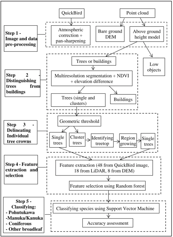
Methods ... 35
Step 1 - Image and data pre-processing ... 36
Step 2 - Distinguishing trees from buildings ... 38
Step 3 - Delineating individual tree crowns ... 39
Step 4 - Feature extraction and selection ... 41
Step 5- Classification and accuracy assessment ... 48
Results and Discussions ... 49
The contribution of different features ... 52
Conclusion ... 54
REFERENCES ... 56
CHAPTER 4 AN EVALUATION OF DIMENSIONALITY REDUCTION AND CLASSIFICATION TECHNIQUES FOR IDENTIFYING TREE SPECIES USING INTEGRATED QUICKBIRD IMAGERY AND LIDAR DATA ... 61
Introduction ... 61
Materials ... 62
Study area and data sets ... 62
Methods ... 63
Dimensionality reduction methods ... 66
Classification techniques ... 68
Validation and comparison method ... 71
Results and Discussions ... 71
Comparison of dimensionality reduction and non-dimensionality reduction for the different classifiers ... 72
Comparing the performance of different classifiers using different training sample sizes and no DR ... 75
Comparing the performance of the best combinations of classifier and DR (or no DR) ... 76
Conclusion ... 79
CHAPTER 5 MONITORING MANGROVE BIOMASS CHANGE IN VIETNAM USING SPOT IMAGES AND AN OBJECT-BASED APPROACH
COMBINED WITH MACHINE LEARNING ALGORITHMS ... 85
Introduction ... 86
Materials ... 88
Study area ... 88
Field data collection ... 89
Image data ... 91
Methods ... 91
Image data pre-processing... 92
Classifying different mangrove associations ... 93
Estimating biomass ... 95
Accuracy assessment ... 101
Results and Discussion ... 101
Classification results ... 101
Variable importance ... 104
Variable selection for the final three RF models ... 105
Biomass distribution and change between 2000 -2011 ... 108
The role of different feature variables for predicting biomass ... 110
Conclusion ... 111
REFERENCES ... 113
CHAPTER 6 DISCUSSION AND CONCLUSION ... 119
Key questions addressed by this research ... 119
Limitations ... 121
Implications for mapping vegetation and future research ... 122
Overall conclusion ... 123
REFERENCES ... 125
REFERENCES ... 127
APPENDICES ... 141
APPENDIX 1 Co-authorship form ... 142
APPENDIX 2 Co-authorship form ... 143
LIST OF FIGURES
Figure 1.1. The sequence of image analysis techniques and the choices available 2 Figure 2.1. The (a) panel shows the linear SVM separable case while the (b) panel shows the linearly non-separable case. Source: adapted from Hastie et al. (2009).
... 20
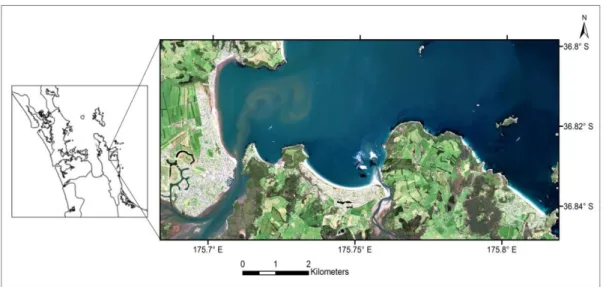
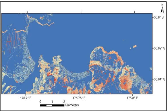
Figure 3.1. QuickBird image of the Coromandel study area. The coordinate is in NZTM2000 projection system. ... 34
Figure 3.2. Workflow of tree species classification ... 36
Figure 3.3. The LiDAR derived height above bare ground model ... 37
Figure 3.4. Decision steps for distinguishing trees and buildings ... 39
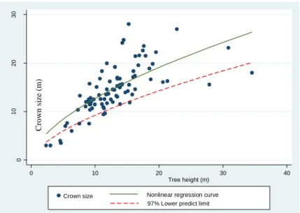
Figure 3.5. The relationship between tree crown size and height ... 40
Figure 3.6. a) A subset image showing crown overlap. b) Segmentation of the image - red polygons represent the ground reference crowns and the blue polygons representing automatic segmentation ... 41
Figure 3.7. The effect of different ntree and mtry values on the performance of RF measured by OOB estimate of error rate using only QuickBird data ... 45
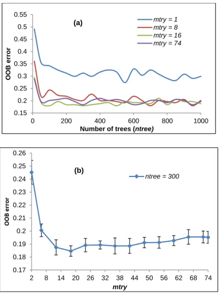
Figure 3.8. The effect of different ntree and mtry values on the performance of RF measured by OOB estimate of error rate using both QuickBird and LiDAR data. ... 46
Figure 3.9. The importance of different features measured by mean decrease accuracy (a) using spectral data (b) using both spectral and LiDAR data. ... 47
Figure 3.10. Box-and-whisker plot showing the statistics of reflectance of different tree species across 4 multi-spectral bands ... 53
Figure 3.11. Box-and-whisker plot showing the statistics of the standard deviation of intensity of all returns of different tree species... 53
Figure 3.12. Box-and-whisker plot showing the statistics of the maximum height of all returns of different tree species ... 54
Figure 4.1. Work flow of mapping tree species using dimensionality reduction and classification techniques... 64
Figure 4.2. Individual tree crowns are represented by polygons. ... 64
Figure 4.3. Classification accuracy (OA) of NB, LR, RF, and SVM with different DR and no DR using a range of training samples per class ... 74
Figure 4.4. Classification accuracy (OA) of NB, LR, RF, and SVM with different training sizes per class with no DR ... 75
xiv
Figure 4.5. The classification accuracy of the best combination of classifier and DR (or no DR) for different training sample size per class. Note: the DR (or no DR) changes with the sample size. ... 79 Figure 5.1. SPOT4 image of the Cangio study area. The coordinate is in WGS 1984 UTM zone 48N projection system. ... 89 Figure 5.2. A workflow of estimating ABG in the Cangio mangrove forest from SPOT data and ground inventory data. ... 92 Figure 5.3.The RMSEOOB is stable after ntree = 1000 for all three cases: spectral +
texture + vegetation association type + vegetation indices (123 variables); spectral + texture + vegetation indices (122 variables); and spectral + vegetation indices (10 variables) used respectively. ... 100 Figure 5.4. Mangrove classification map of the Cangio in: (a) 26th March 2000 and (b) 24th February 2011 ... 102 Figure 5.5. The importance of different features measured by %InMSE (the percentage increase in the mean squared error) determined from 100 runs of the RF for: (a) all 123 variables used (spectral + texture + VI + vegetation association type); (b) 122 variables used (spectral + texture + VI); (c) 10 variables (spectral + VI). ... 105 Figure 5.6. The number of variables used and the average RMSE of models based on 100 times of 10-fold cross validation: (a) all 123 variables; (b) 122 variables; (c) 10 variables. ... 106 Figure 5.7. Plots of the observed and predicted biomass values using RF with a) Model 1; b) Model 2; c) Model 3 ... 108 Figure 5.8. Biomass map of the Cangio mangrove forest: (a) 2000 derived from SPOT4 and (b) 2011 derived from SPOT5 ... 109
LIST OF TABLES
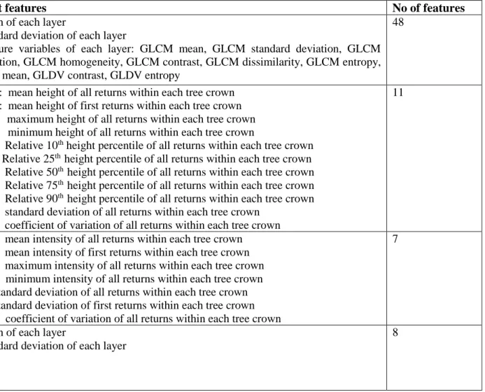
Table 3.1. Ground-truthed data ... 35 Table 3.2. Image object features used for classifications... 43 Table 3.3. Confusion matrix of classification accuracies obtained through RF feature selection and SVM classifier... 50 Table 3.4. Confusion matrix of classification accuracies obtained through SVM classifier without feature selection ... 51 Table 4.1. Image object features were used for classifications ... 65 Table 4.2. Comparison between four different classifiers combined with four different DR methods and no DR. Paired t-test (corrected) between the use of DR and no DR at 0.05 significance level from 10-fold CV repeated 5 times. Note: (b) and (w) denote that the result was statistically better or worse respectively than the no DR, while (-) denotes that there was no significant difference. ... 73 Table 4.3. Comparing NB, LR, RF, and SVM using all features and different training set sizes with 10-fold CV repeated 5 times and paired t-tester (corrected) at 0.05 significance level. Note: Bolded OA and Kappa scores indicate the highest performance, b and w denote the result is statistically better or worse than the classifier compared; while - denotes there is no significant difference between classifiers. ... 76 Table 4.4. Comparing the best classification accuracy of NB, LR, RF, and SVM and different training set sizes with 10-fold CV repeated 5 times and paired t-tester (corrected) at 0.05 significance level. Note: Bolded OA and Kappa scores indicate the highest performance, b and w denote that the result is statistically significantly better or worse respectively than the classifier compared; while - denotes there is no significant difference between classifiers. ... 78 Table 5.1. Species-specific biomass allometric equations for the Cangio mangrove forest ... 90 Table 5.2. Descriptive statistics of biomass plots ... 90 Table 5.3. Variables for calculating biomass (spectral and texture variables were also used for classification) ... 96 Table 5.4. Confusion matrix of classification accuracies obtained through SVM classifier in 2000 and 2011 ... 103 Table 5.5. Summary of settings for Random Forest Models ... 107
xvi
Table 5.6. Calibration and validation results ... 107 Table 5.7. General descriptive statistics of AGB in the Cangio mangrove forest in the years 2000 and 2011 ... 109
LIST OF ACRONYMS & ABBREVIATIONS
AD Allocation Disagreement
AGB Above-Ground Biomass
ANN Artificial Neutral Network
ATCOR Atmospheric Correction Algorithm
CFS Correlation-Based Feature Selection
CHM Canopy Height Model
CMM Canopy Maxima Model
DBH Diameter at Breast Height
DEM Digital Elevation Model
DR Dimensionality Reduction
DT Decision Tree
EVI Enhanced Vegetation Index
FLAASH Fast Line-of-sight Atmospheric Analysis of Hypercubes
GLCM Grey-Level Co-occurrence
GLDV Gray-Level Difference Vector
GPS Global Positioning System
INFOGAIN Information Gain
K Kappa coefficient of agreement
LiDAR Light Detection And Raging
LR Logistic Regression
MIR Mid-Infrared
ML Maximum Likelihood
MSAVI Modified Soil-Adjusted Vegetation Index
NB Naïve Bayes
NDVI Normalized Difference Vegetation Index
NDWI Normalized Difference Water Index
NIR Near InfraRed
OA Overall Accuracy
OBIA Object-based Image Analysis
OOB Out-Of-Bag
OSAVI Optimized Soil-Adjusted Vegetation Index
xviii
PCA Principal Component Analysis
QD Quantity Disagreement
RBF Radial Basis Function
RF Random Forest
SAVI Soil-Adjusted Vegetation Index
SPOT Satellite Pour l'Observation de la Terre
SS Sequential Selection
SVM Support Vector Machine
TD Total Disagreement
TWI Topographical Wetness Index
CHAPTER 1
INTRODUCTION AND THE RESEARCH CONTEXT
The motivation for this research was to develop techniques for monitoring change to coastal vegetation using remote sensing. Natural and anthropogenic disturbances of coastal vegetation are a major issue. Monitoring the spatial extent of coastal vegetation is an important step in understanding these disturbances, and remote sensing technology is a useful tool for providing such information. This thesis researches the use of advanced remote sensing techniques, including object-based image analysis and machine learning algorithms for coastal vegetation.
The first sections of this introduction chapter provide an overview of previous remote sensing research and what this thesis will do to address the gaps in the literature. Next sections provide the aim and scope of this research. The final section provides information about thesis structure and chapter outlines.
Remote sensing research
Remote sensing has been demonstrated to be cost efficient and effective for many practical applications such as biodiversity monitoring, agriculture planning, and forest fire control and management. Remote sensing is a rapidly changing technology due to new data sources becoming available as well as advancing image analysis techniques.
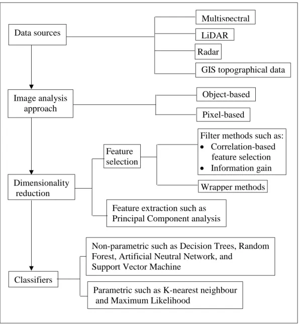
Image analysis is a combination of different data sets, pre-processing, and image classification techniques. Figure 1.1 shows the sequence of these techniques and the choices available, which are represented on the left of this Figure as data sources, image analysis, dimensionality reduction, and classifiers. These techniques interact and can impact on the accuracy of the final classification. For example, using the object-based image analysis for high resolution multispectral data can extract more input variables for classification such as contextual variables than the pixel-based approach. The large number of input data requires pre-processing steps using dimensionality reduction methods to obtain higher classification accuracy. The preferred combination of analysis techniques therefore requires research.
2
Figure 1.1. The sequence of image analysis techniques and the choices available
Traditionally remotely sensed data has mainly focused on multispectral images, but now there is a wide range of data sets that can be used in remote sensing, which includes hyperspectral images, LiDAR, and RADAR data, as well as GIS topographical data that provides environmental context. Spectral data can now be combined with tree height and shape, as well as landform and wetness indices. Using simultaneously multiple data sets introduces new challenges in image analysis and this research investigates whether such data sets improve image classification accuracy.
As well as advances in the number and quality of available data sets, techniques for image analysis have also improved. Traditionally images have been classified at the
Data sources
Multispectral LiDAR Radar
GIS topographical data
Image analysis approach Object-based Feature selection Dimensionality reduction Classifiers
Filter methods such as: • Correlation-based feature selection • Information gain
Feature extraction such as Principal Component analysis
Wrapper methods Pixel-based
Non-parametric such as Decision Trees, Random Forest, Artificial Neutral Network, and
Support Vector Machine
Parametric such as K-nearest neighbour and Maximum Likelihood
pixel level but a more sophisticated technique is the use of object-based image analysis (OBIA; see chapter 2 for details). The OBIA first joins pixels into objects (this process is known as segmentation), and then classification is performed on these objects using the diversity of spectral, textural, and contextual information. In contrast to the pixel-based approach, the OBIA exploits various information simultaneously such as spectral, spatial, shape, textural, and contextual information. The effectiveness of using OBIA combined with multiple data sets depends on the classification targets and the types of data sources available. However, there is no general framework about how to integrate OBIA and multiple data sets for mapping vegetation; therefore research is required. In addition, the level of segmentation used depends on the data and the objects being identified. This level needs to be investigated to produce the most optimal results.
Combining multiple datasets can result in high computational demand as well as feature redundancy that compromise classification performance. Therefore, pre-processing the data using dimensionality reduction methods is often done to not only reduce processing time but also improve the classification accuracy. There are many dimensionality reduction techniques to choose from such as Correlation-based feature selection filter, Information gain, and Wrapper methods. Choosing the best dimensionality reduction methods is important for improving classification accuracy and will be explored in this research.
In addition to the above techniques, several image classification algorithms have been developed. These include parametric classifiers such as Maximum Likelihood, and K-nearest neighbour, as well as non-parametric methods such as Decision Trees, Artificial Neutral Network, Random Forest, and Support Vector Machine (see details in Chapter 2). The choice of classification algorithms depends on the data properties and this is investigated to determine which is best for classification accuracy.
Remote sensing of coastal vegetation
Another aspect of remote sensing research is developing new applications of remote sensing such as single tree mapping and biomass estimation. The performance of different remote sensing techniques, such as described previously, will vary with
4
different vegetation types. It is therefore necessary to choose a particular context for the research as it is not practical to research their accuracy with all the different vegetation types. This thesis focuses on using remote sensing techniques for mapping coastal vegetation and testing their accuracies. The reason for choosing coastal vegetation is twofold. Firstly the research was supported by an international collaboration between the University of Waikato in NZ and the University of Bremen in Germany, called INTERCOAST. This collaboration focuses on coastal research.
The second reason was because of the importance of coastal vegetation. Coastal ecosystems such as dunes, mangrove forests, salt marshes, and coral reefs provide several important services such as purifying the water from human wastes and pollutants, preventing coastal erosion, and minimizing the impact of natural disasters such as flood, tsunamis and hurricane (Tanaka et al., 2007; Wang and Wang, 2010). In addition, coastal ecosystems provide scenic beauty and recreation (Álvarez-Molina et al., 2012). However, those ecosystems are facing increased natural and anthropogenic disturbances such as climate change, sea level rise, storms, land use change and encroachment by urban development (Álvarez-Molina et al., 2012; Wang and Wang, 2010). Providing accurate up-to-date information about the characteristics of the coastal vegetation such as the presence of individual species, distribution, and biomass is necessary to help managers and policy makers decide on appropriate conservation and restoration strategies within a restricted time span.
Coastal vegetation can be mapped using a range of methods. Traditional vegetation mapping methods such as field surveys or aerial photography interpretation are time-consuming, costly and provide inconsistent results (Castillejo-González et al., 2009; Xie et al., 2008). Compared to traditional field surveys, the use of satellite remotely sensed data has many advantages such as significantly lower costs; it is also quicker and more suitable for use over extensive areas (Castillejo-González et al., 2009; Xie et al., 2008). Given these strengths, remote sensing data have been commonly used for identifying coastal vegetation and measuring its physical characteristics.
Many studies using remote sensing have mapped vegetation at a coarse spatial resolution data which is defined by Xie et al. (2008) as pixels with ground sampling distance of 30 m or greater and identified vegetation types that often include several different species. Given the desire to provide the most detailed and accurate results, vegetation maps should use high quality remotely sensed data and advanced image analysis techniques. This research thus focuses on mapping single trees in New Zealand, where high quality data is available.
Although this study uses high quality data, such as LIDAR and QuickBird images, for New Zealand, it is important to be mindful that many developing countries do not have access to such data because of the expense. Developing countries also face high environmental pressures and have a need for vegetation monitoring. Therefore, research on remote sensing should consider how best to utilise low resolution images, such as Landsat and SPOT, which are considerably cheaper. This research modified the methodology developed in New Zealand and applied this to the context of developing countries lower spatial resolution data sources.
Aim of this research
The main objective of this research is to evaluate a range of remote sensing techniques for mapping coastal vegetation as accurately as possible, including the best combination of techniques. This vegetation mapping includes mapping the location of individual trees in New Zealand as well as calculating biomass of mangrove forests in Vietnam.
Specific research questions
1. What levels of segmentation are required to separate individual tree crowns/mangrove associations from other land-cover types such as grasslands, buildings, and water?
2. Which dimensionality reduction methods improve the accuracy of vegetation classification or biomass prediction?
3. Which classifier algorithms should be used for identifying coastal vegetation?
4. Does the combination of spectral and GIS derived data improve the accuracy of vegetation classification and biomass prediction?
6
Scope of this research
This study will use a unique combination of GIS data, remotely sensed images, OBIA with different dimensionality reduction and classification techniques that have never been used before for mapping tree species and estimating biomass. Improving the vegetation classification accuracy is the main goal of this research. The accuracy will be compared with other vegetation mapping studies conducted elsewhere in the world.
Two study areas have been chosen for this research – a coastal site in NZ for which higher spatial resolution data is available and a coastal site in Vietnam that has lower spatial resolution data sources. These two countries provided the opportunity to investigate whether the object-based approach with various classifiers is widely applicable for different types of environments and vegetation species.
Case study in New Zealand – Coromandel Peninsula
The New Zealand site is the Coromandel Peninsula. The site is characterized by different land cover types including built-up area, urban parkland/open space, sand or gravel, coastal broadleaved species of scrub or scrublands, pine forests, manuka and/or kanuka, and pohutukawa forests on the coast (Humphreys and Tyler, 1990; Weeks et al., 2009).
Pohutukawa, one of the best-known native trees in New Zealand, is a coastal species and found mainly in northern New Zealand (Bergin and Hosking, 2006; Simpson, 2005). Pohutukawa has cultural significance to Maori including medicinal uses. It has also provided timber for boat building. At present, it is used for honey production as well as cosmetic and cleaning products (Bergin and Hosking, 2006; Simpson, 2005). Regarding its ecological and environmental functions, it helps stabilize soil on eroding or unstable areas and provides habitat and resources to plant and animal associates such as tui and bellbird (Bergin and Hosking, 2006). Despite such benefits, the number of Pohutukawa trees has considerably declined in the past due to fires and land clearance (Bergin and Hosking, 2006; Simpson, 2005). Unfortunately, this decrease is continuing at present, mainly due to possum and herbivore browsing (Bergin and Hosking, 2006; Bylsma, 2012). Recently
Pohutukawa has been considered to be at risk from myrtle rust. Therefore, counting the trees which is the first step at monitoring impacts such as possum browsing is necessary to help managers develop appropriate conservation strategies. These tasks can be done effectively and economically using remote sensing data combined with the object-based approach to identify individual trees. A map showing individual tree locations of Pohutukawa would be a first for NZ and would generate considerable interest. It is expected that the method developed will be applicable in similar locations throughout NZ.
The Coromandel Peninsula has been chosen because: 1) LIDAR and QuickBird data sets (high spatial resolution) are available, 2) there is a range of coastal vegetation including Pohutukawa, conifers, and exotic species, and 3) it is accessible by car so that ground-truth data can be collected easily.
Case study in Vietnam – Cangio mangrove forests
The Vietnam site is the Cangio mangrove forests. The Cangio mangrove forest is located in Cangio District - one of 24 districts of Ho Chi Minh City - covering an area of about 72 000 ha. In January 2000, the Cangio mangrove forest was recognized as the first biosphere reserve in Vietnam. This reserve consists of 60% planted and 40% natural forests (Kuenzer and Tuan, 2013). There are more than 200 species of fauna and more than 52 species of flora, so it is considered to have high biodiversity (Nguyen, 2006). Besides those types of vegetation, the research area includes shrimp ponds, bare lands, and muddy flats. Mangroves in Cangio have been facing the threat of increased coastal erosion as a result of the transit of large cargo ships, the ever expanding aquaculture and salt farming activities, and the negative impacts of socio-economic transformation (Kuenzer and Tuan, 2013). This site has been chosen because: 1) SPOT images and Digital Elevation data (DEM) are freely available; 2) there are various mangrove species; 3) there is a range of GIS data available; and 4) mangrove forest in Cangio is extensive and the methodology developed by this research can be evaluated in different environments.
8
Thesis structure and chapter outlines
This thesis consists of six chapters – this general introductory chapter (Chapter 1), a literature review of advanced image analysis techniques (Chapter 2), three chapters written as manuscripts for publication (Chapters 3, 4, and 5), and a concluding chapter (Chapter 6) that provides discussions and a final conclusion. Because the research chapters 3, 4, and 5 have been submitted to different journals, they follow different specific formatting and referencing styles appropriate to each journal. However, changes have been made in the formats of the individual chapters to maintain the overall consistency of the overall thesis.
Chapter 2 – “A literature review of advanced image analysis techniques for mapping vegetation”.
Chapter 2 clarifies the advantages of OBIA compared to the traditional pixel-based approach. It also reviews different machine learning algorithms for classifying vegetation and predicting biomass. It enables the discovery of knowledge gaps in the use and combination of existing techniques that the thesis seeks to fill.
Chapter 3 - “Combining QuickBird, LiDAR, and GIS topography indices to identify a single native tree species in a complex landscape using an object-based classification approach”.
Chapter 3 is a peer-reviewed paper published as “Pham, L.T.H, Brabyn, L., Ashraf, S., 2016. Combining QuickBird, LiDAR, and GIS topography indices to identify a single native tree species in a complex landscape using an object-based classification approach. International Journal of Applied Earth Observation and Geoinformation 50, 187-197”. http://dx.doi.org/10.1016/j.jag.2016.03.015
The chapter investigates the benefits of combining a range of techniques to identify individual tree species. A QuickBird image and low point density LiDAR data for a coastal region in New Zealand were used to examine the possibility of mapping individual Pohutukawa trees, which are regarded as an iconic tree in New Zealand. This chapter shows how combining LiDAR and spectral data improves classification for Pohutukawa trees.
Chapter 4 - “An evaluation of dimensionality reduction and classification techniques for identifying tree species using integrated QuickBird imagery and LiDAR data”
Chapter 4 is a paper submitted to the “IEEE Transactions on Geoscience and Remote Sensing” Journal. This chapter investigates and compares tree species classification performance for a variety of classification schemes (Naïve Bayes, Logistic Regression, Random Forest, and Support Vector Machine), combined with various dimensionality reduction methods (Correlation-based feature selection filter, Information Gain, Wrapper methods, and Principle component analysis). This chapter concludes that the SVM and RF achieve highest classification accuracy, and dimensionality reduction should be applied prior to the classification step to make the classifier algorithms run faster and/or achieve higher classification accuracy.
Chapter 5 - “Monitoring mangrove biomass change in Vietnam using SPOT images and an object-based approach combined with machine learning algorithms”. Chapter 5 is a peer-reviewed paper published as “Pham, L.T.H., Brabyn, L., 2017. Monitoring mangrove biomass change in Vietnam using SPOT images and an object-based approach combined with machine learning algorithms”. ISPRS Journal of Photogrammetry and Remote Sensing 128, 86 -97”. http://dx.doi.org/10.1016/j.isprsjprs.2017.03.013
The chapter extends the applications of an object-based approach for measuring the biomass change between 2000 and 2011 of mangrove forests in the Cangio region in Vietnam. Firstly, it uses object-based image analysis and Support Vector Machine classifier for identifying different mangrove types. Random Forest regression algorithms are then used for modelling and mapping biomass. This chapter concludes that the integration of spectral, vegetation association type, texture, and vegetation indices obtains the highest accuracy (R2adj = 0.73).
Chapter 6 – “Discussion and Conclusion”
This final chapter synthesises resultsgiven in previous chapters, and summarises the answers to the research questions. This chapter recaps the contribution of this
10
research in establishing new knowledge for remote sensing of vegetation. Limitations of this research are discussed, including suggestions for future research that address these limitations.
REFERENCES
Álvarez-Molina, L.L., Martínez, M.L., Pérez-Maqueo, O., Gallego-Fernández, J.B., Flores, P., 2012. Richness, diversity, and rate of primary succession over 20 year in tropical coastal dunes. Plant Ecology 213(10), 1597-1608.
https://doi.org/10.1007/s11258-012-0114-5
Bergin, D., Hosking, G., 2006. Pohutukawa-ecology, establishment, growth and management. New Zealand Indigenous Tree Series No. 4. New Zealand Forest Research Institute, Rotorua.
Bylsma, R.J., 2012. Structure, composition and dynamics of Metrosideros excelsa (pōhutukawa) forest, Bay of Plenty, New ZealandUniversity of Waikato. Castillejo-González, I.L., López-Granados, F., García-Ferrer, A., Peña-Barragán,
J.M., Jurado-Expósito, M., de la Orden, M.S., González-Audicana, M., 2009. Object- and pixel-based analysis for mapping crops and their agro-environmental associated measures using QuickBird imagery. Computers
and Electronics in Agriculture 68(2), 207-215.
https://doi.org/10.1016/j.compag.2009.06.004
Humphreys, E.A., Tyler, A.M., 1990. Coromandel Ecological Region: survey report for the Protected Natural Areas Programme. Department of Conservation, Waikato Conservancy.
Kuenzer, C., Tuan, V.Q., 2013. Assessing the ecosystem services value of Can Gio Mangrove Biosphere Reserve: Combining earth-observation- and household-survey-based analyses. Applied Geography 45, 167-184.
https://doi.org/10.1016/j.apgeog.2013.08.012
Nguyen, H.N., 2006. The environment in Ho Chi Minh City harbours, in: Wolanski, E. (Ed.), The Environment in Asia Pacific Harbours. Springer, Dordrecht, The Netherlands, pp. 261-291.
Simpson, P., 2005. Pohutukawa and Rata: New Zealand's Iron-Hearted Trees. Te Papa Press, Wellington, New Zealand.
Tanaka, N., Sasaki, Y., Mowjood, M.I.M., Jinadasa, K.B.S.N., Homchuen, S., 2007. Coastal vegetation structures and their functions in tsunami protection: experience of the recent Indian Ocean tsunami. Landscape Ecol Eng 3(1), 33-45. https://doi.org/10.1007/s11355-006-0013-9
Wang, Y., Wang, J., 2010. Remote sensing of coastal environments: An overview, in: Wang, Y. (Ed.), Remote Sensing of Coastal Environments. CRC Press, Boca Raton, FL, pp. 1-24.
Weeks, E., Newsome, P., Shepherd, J., 2009. National SPOT-5 Image Ortho-rectification and Reflectance Standardisatio: Final Project Report Landcare Research Contract Report: LC0809/102, Palmerston North, New Zealand. Xie, Y., Sha, Z., Yu, M., 2008. Remote sensing imagery in vegetation mapping: a
review. Journal of Plant Ecology 1(1), 9-23.
CHAPTER 2
A LITERATURE REVIEW OF ADVANCED IMAGE ANALYSIS TECHNIQUES FOR MAPPING VEGETATION
2.1 Introduction
Remote sensing techniques cover a wide range of image preparation, classification, and accuracy assessment techniques. The emergence of various remote sensing data sources requires new and advanced image processing techniques to use these data sets efficiently. An overview of different types of image analysis techniques used for mapping vegetation can be found in many articles and remote sensing text books such as Chuvieco (2016), Houborg et al. (2015), Pettorelli et al. (2014), and Wang (2009). As stated in the introduction chapter this thesis focuses on advanced image analysis techniques. Therefore this review chapter focuses on just these techniques and the methods that are common to all three chapter/papers. This includes object based classification, integration of GIS and remotely sensed data, classifiers, and accuracy assessment. The subsequent chapters/papers summarise the main points of this review in light of the restriction imposed by the publication format as well as review specialised methods that are relevant to the particular chapter/paper. These specialised methods include LiDAR processing, treetop identification, biomass estimation, allometric functions, and dimensionality reduction techniques. 2.2 Pixel-based versus object-based approach
Two common categorial image analysis approaches are pixel-based and object-based analysis (Aguirre-Gutiérrez et al., 2012). While the pixel-object-based analysis has long been the main approach used in remote sensing studies, the object-based image analysis has become increasingly popular over the last decade (Blaschke, 2010; Duro et al., 2012). A pixel-based analysis approach assigns an individual pixel into one category (Liu and Xia, 2010) while an object-based approach operates on objects which are groups of homogenous and contiguous pixels (Liu and Xia, 2010). Compared to the pixel-based technique, the OBIA has many advantages. Firstly, shifting the classification units from pixels to image objects decreases the intra-class spectral variability and removes the “salt-and-pepper” problem which is usual
14
in pixel-based classification of high spatial resolution imagery (Gao et al., 2007; Liu and Xia, 2010; Yu et al., 2006). Secondly, the OBIA integrates various features of image objects. It can use not only the spectral properties but also spatial and contextual information into the classification process, which may be able to perform the classification more accurately (Blaschke, 2010; Blaschke et al., 2014a; Gao et al., 2007; Han et al., 2014; Ouyang et al., 2011). Thirdly, the object-based approach with multi-scale segmentation and hierarchical structure of the classification scheme will provide detailed information at different levels of landscape such as from individual trees to forests (Mishra and Crews, 2014). Thanks to these flexibility characteristics, the cost for producing many products and updating information at different levels of the landscape is reduced significantly. However, one of the drawbacks of object-based image analysis is that the segmentation process and the calculation of the topological relationships between objects can consume a large amount of computer memory (Liu and Xia, 2010; Whiteside et al., 2011). In addition, there are no objective methods to choose parameters for producing image objects (Jakubowski et al., 2013; Liu and Xia, 2010; Whiteside et al., 2011). Other disadvantages are that the software is expensive and has a steep learning curve.
Many studies showed that the OBIA performed better than the pixel-based methods using a great variety of remote sensing imagery for mapping vegetation. For example, Ouyang et al. (2011) compared pixel-based and object-based analysis using QuickBird imagery and different classification models for mapping saltmarsh plants. The results indicated that OBIA achieved higher overall accuracy (87%) than the pixel-based approach (82%). Moreover, there was no “salt and pepper” in the map created from object-based classification approaches. Ghosh and Joshi (2014) used WorldView-2 imagery and different classification algorithms to map bamboo patches in West Bengal, India. Their method combined both the OBIA and a Support Vector Machine classifier, which produced 91% accuracy while the pixel-based classification scheme was only 80% accurate. Similarly, Fu et al. (2017) showed that the object-based Random Forest algorithm improved the overall accuracy (OA) between 3%-10% when compared to pixel-based classifications for wetland vegetation using high spatial resolution Gaofen-1 satellite image, L-band PALSAR and C-band Radarsat-2 data.
The OBIA outperforms pixel-based analysis for not only high but also medium resolution satellite imagery. For instance, Whiteside et al. (2011) used ASTER data to map land cover in the tropical north of the Northern Territory of Australia. The OA of using the object-oriented approach was statistically significantly greater than that of the pixel-based approach. Similarly, Myint et al. (2008) found that an object-based approach with the lacunarity technique for Landsat Thematic Mapper data was more effective in identifying three types of mangrove species than a pixel-based classifier. The OA of the object-oriented classifier was significantly higher than that of the pixel-based classifier (94.2% and 62.8% respectively).
Although the above studies found that the OBIA obtained more accurate results than pixel-based methods, the pixel-based approach may achieve similar or sometimes more accurate classification results for certain land cover categories (Duro et al., 2012; Flanders et al., 2003). In such cases, the combination of two approaches can produce the best results. Wang et al. (2004a) demonstrated that the OA of mangrove maps created from very high-resolution IKONOS imagery was improved when combining pixel-based and object-based classifications. Similarly, Aguirre-Gutiérrez et al. (2012) compared the land cover classification results among pixel-based, object-based, and the combined object-based and pixel-based classification using medium resolution imagery (Landsat ETM+). The result showed that the combination method delivered the best results. Li et al. (2013) also illustrated that the hybrid of image segmentation and pixel-based classification for land cover classification outperformed the use of object-based or pixel-based approach alone.
2.3 Object-based image segmentation
A defining step in OBIA is image segmentation (Kim et al., 2009a; Lang, 2008), which divides an image into contiguous, separate and homogeneous areas. These areas are called image objects (Blaschke et al., 2004; Blaschke et al., 2014b; Duro et al., 2012), which are then classified into different categories using a range of classifiers (reviewed in the next section). The quality of segmentation will affect the accuracy of the classified image (Kim et al., 2009a; Liu and Xia, 2010). The segmenting process can produce meaningful image objects at different scales of the landscape (granularity), which enables multiple features to be extracted from a
16
single dataset (Burnett and Blaschke, 2003; Lang and Langanke, 2006; Mishra and Crews, 2014).
Image segmentation methods can be divided into three categories, including point-based or pixel-point-based (e.g. grey-level thresholding), edge-point-based (e.g. edge detection techniques), and region-based (Blaschke et al., 2004; Pal and Pal, 1993; Van Coillie et al., 2007). Point-based methods gather pixels in a feature space using thresholds and clusters (Yu et al., 2006). Edge-based methods determine boundaries between image objects using edge detection algorithms based on changes in values (Blaschke et al., 2004; Yu et al., 2006). Region extraction can be divided into region growing, region dividing, and their combinations (Blaschke et al., 2004; Yu et al., 2006). The region growing method starts with a set of seed pixels, which are then merged to adjacent pixels that are similar (Ke and Quackenbush, 2011). This process of growing continues until a threshold is reached, and defined by specified homogeneity criteria (Blaschke et al., 2004). For segmenting individual tree crowns, various semi- and fully-automated methods have been developed and can be generally categorized into: template matching (Korpela et al., 2007; Olofsson et al., 2006); valley following (Leckie et al., 2003); watershed segmentation (Chen et al., 2006); and region growing (Bunting and Lucas, 2006; Li et al., 2012; Zhen et al., 2014). The region growing method outperformed other methods, e.g., valley-following (Hussin et al., 2014; Larsen et al., 2011), and template matching (Larsen et al., 2011) in a mixed forest.
2.4 Combining GIS data with remotely sensed data
The OBIA provides the possibilities to integrate GIS techniques and image processing to use data effectively and improve classification. This is especially useful for situations where shape or neighbourhood relations are distinctive and spectral properties are not (Blaschke et al., 2014b). For example, old meandering river beds can have a range of land cover possibilities such as remaining water filled in by sediment or overgrown by vegetation. The mixed spectral properties in this case limits the meanders identification. However, the unchanged shape of the meander provides a unique property to distinguish it from its land cover appearance (Blaschke et al., 2014b).
The integration of GIS data with remotely sensed data has been used in many studies. Han et al. (2014) used the linkages between vegetated objects at different scales to identify land cover types in shadow areas for Moso bamboo forest. Similarly, MacFaden et al. (2012) combined multispectral imagery and LiDAR data using OBIA with contextual analysis to distinguish urban tree canopy from other land cover types. The contextual analysis in their research focused on the relationship between individual objects and their neighbours. MacFaden et al. (2012) identified tree canopy with accuracy that exceeded 90%. Yu et al. (2006) also used integrated Digital Airborne Imaging System imagery and topographic data with the object-based approach for detailed vegetation classification in Northern California. They pointed out that topographic information such as slope, aspect, and distance to water courses contributed significantly for vegetation classification besides spectral and texture features derived from airborne imagery. Likewise, Blaschke et al. (2014a) showed that the combination of difference variables from satellite images with GIS variables such as slope and flow direction derivatives can detect and delineate landslides more accurately than using a single data source.
2.5 Classification algorithms
Choosing suitable classification algorithms is important to improve classification accuracy (Lu and Weng, 2007; Otukei and Blaschke, 2010). There are two main types of classification algorithms - supervised and unsupervised classification (Lu and Weng, 2007). Commonly used supervised classification techniques include Maximum Likelihood (ML), Minimum Distance, Artificial Neutral Network (ANN), and Support Vector Machine (SVM); while unsupervised methods include K-Means and ISODATA (Ghosh and Joshi, 2014; Lu and Weng, 2007). Classification algorithms are also divided into non-parametric methods such as Decision Tree (DT), ANN, and SVM,and parametric methods such as ML and K-nearest neighbour (Ghosh and Joshi, 2014; Lu and Weng, 2007; Yu et al., 2006). The most commonly used parametric classifier in remote sensing is the ML because it is widely available in image-processing software programmes (Ghosh and Joshi, 2014; Lu and Weng, 2007). However, the parametric approach assumes that the image data are normally distributed. Such assumption is often not guaranteed, especially in complex landscapes (Löw et al., 2015; Lu and Weng, 2007). This
18
assumption error is more serious in circumstances where training samples are not adequate, unrepresentative, or multimode distributed (Cracknell and Reading, 2014; Lu and Weng, 2007).
In contrast to parametric classifiers, non-parametric classifiers do not need an assumption of normal distribution of the dataset (Löw et al., 2015; Lu and Weng, 2007). This flexible characteristic of non-parametric classifiers allows integration of spectral and ancillary data into a classification process. Several previous studies have shown that non-parametric classifiers can produce better results than parametric classifiers in complex landscapes (Cracknell and Reading, 2014; Ghosh and Joshi, 2014). Neural Networks, DT, SVM, and Random Forest (RF) are the most common non-parametric classifiers (Löw et al., 2015; Lu and Weng, 2007; Raczko and Zagajewski, 2017).
Many studies compare the performance between parametric classifiers and non-parametric classifiers and amongst non-non-parametric classifiers. There is no consensus as to which method is the best practice. In general, RF and SVM perform better than ANN and MLC, especially when there is a limited number of training samples and many different classes (Cracknell and Reading, 2014). Ghosh and Joshi (2014) compared the performance among kernel based SVM, ensemble based RF and parametric ML classifiers in both pixel-based and object-based classification approaches for mapping bamboo patches in West Bengal India with WorldView 2 imagery. They showed that SVM produced higher accuracy than RF and ML classifiers while ML classifiers ran faster than SVM and RF. Similarly, Dalponte et al. (2012) identified tree species in the Southern Alps, Italy using the fused multispectral/hyperspectral images and LiDAR data and two non-parametric classifiers (SVM and RF). Their results showed that SVM provided better results than RF. Dalponte et al. (2012) explained that the unbalanced number of training samples among tree species classes may lead to the poor performance of RF. Duro et al. (2012) mapped agricultural landscapes in western Canada using SPOT-5 HRG imagery (medium spatial resolution multi-spectral imagery). Duro et al. (2012) compared the performance between three non-parametric classifiers: DT, RF, and SVM. They found that object-based classification using the DT algorithm had lower overall classification accuracy (88.84%) than the RF (93.39%) and the SVM
(94.21%) classifiers. Furthermore, statistical assessment of the classification results showed that there were statistically significant differences between DT and SVM algorithms and DT and RF algorithms. On the other hand, Otukei and Blaschke (2010) found that DT generally performed better than classifications produced using SVM. Pal (2005) showed that both SVM and RF algorithms produced similar classification accuracies.
Because this thesis mainly uses machine learning SVM and RF algorithms, these are reviewed in detail in the following subsections. The reason why the SVM and RF are used in this thesis is explained in Chapter 3 and 5. Naïve Bayes and Logistic Regressions are reviewed in Chapter 5.
2.5.1 Support Vector Machine
The theory of SVM was developed by Vapnik (1995). The SVM algorithm determines a hyperplane that separates the dataset into a discrete number of classes (Han et al., 2012). The basic theory of SVM is explained by Vapnik (1995) and Hastie et al. (2009) using the following mathematical nomenclature: Given the training data T with N samples: T = {(x1,y1), (x2,y2),…(xn,yn)}, where xi∈ ℝ𝑑and
yi ∈{-1,1}, i=1,2,…,n. With the linear data, the separating hyperplane which
classifies the data input can be written as: 𝑓(x) = wT. x + b = ∑ (wT𝑥
𝑖 + b) 𝑁
𝑖=1 = 0, (2.1)
where 𝑤 is a N-dimensional vector and b is a scalar.
The separating hyperplane satisfies the following constraint in order for data points to lie on the correct side of the margin:
𝑦𝑖𝑓(𝑥𝑖) = 𝑦𝑖(wT𝑥𝑖 + b) ≥ 1, ∀𝑖 (𝑖 = 1, … , 𝑁). (2.2)
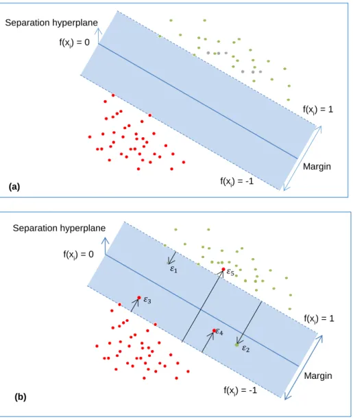
The separating hyperplane which has the maximum distance between the plane and the nearest training data (or the maximum margin) is the optimal separating hyperplane. The nearest data samples that are used to define the margin are support vectors, shown as thick borders (see Figure 2.1).
20
Figure 2.1. The (a) panel shows the linear SVM separable case while the (b) panel shows the linearly non-separable case. Source: adapted from Hastie et al. (2009).
Geometrically, the margin is equal to ‖𝑤‖2 . To maximize the distance between the plane and the nearest training data, ‖w‖ should be minimized. Therefore, the optimal separating hyperplane for classifying two different categories of data can be obtained as a solution to the following optimization problem:
min
w,𝑏‖w‖ (2.3)
subject to the constraint (2.2)
When introducing the slack variables 𝜀𝑖 to intensify the generalization, the optimization problem is modified to:
f(xi) = -1 f(xi) = 1 (a) Separation hyperplane Margin f(xi) = 0 f(xi) = -1 f(xi) = 1 f(xi) = 0 Margin (b) 𝜀1 𝜀2 𝜀3 𝜀5 𝜀4 Separation hyperplane
min
w,𝑏(‖w‖) subject to {
𝑦𝑖(wT𝑥𝑖 + b) ≥ 1 − 𝜀𝑖, ∀𝑖 (𝑖 = 1, … . , 𝑁),
𝜀𝑖 ≥ 0, ∑ 𝜀𝑖 ≤ constant
(2.4)
The slack variables measure the distance between the margin and the data point that lies beyond the correct margin. The problem (2.4) is quadratic with linear inequality constraints, therefore it is a convex optimization problem. For computational convenience, (2.4) is re-expressed in the equivalent form:
min w,𝑏 ( 1 2 ‖w‖ 2) + 𝐶 ∑ 𝜀 𝑖 𝑁 𝑖=1 (2.5) subject to 𝜀𝑖 ≥ 0, 𝑦𝑖(wT𝑥𝑖 + b) ≥ 1 − 𝜀𝑖, ∀𝑖,
where the parameter C replaces the constant in (2.4)
To optimize (2.5), the Lagrange (primal) function is applied:
L (w, b, 𝜀𝑖) = 1 2 ‖w‖ 2+ 𝐶 ∑ 𝜀 𝑖 𝑁 𝑖=1 − ∑𝑁𝑖=1𝛼𝑖[𝑦𝑖(wT𝑥𝑖+ b) − (1 − 𝜀𝑖)] − ∑𝑁𝑖=1𝜇𝑖𝜀𝑖 (2.6)
Setting the derivatives of L with respect to w, b, and 𝜀𝑖 to zero, we get:
w = ∑𝑁𝑖=1𝛼𝑖𝑦𝑖𝑥𝑖, (2.7)
0 = 𝛼𝑖𝑦𝑖, (2.8)
𝛼𝑖 = 𝐶 − 𝜇𝑖, ∀𝑖, (2.9)
Substituting (2.7), (2.8), (2.9) into (2.6), we get the Lagrangian dual problem: maximize L (𝛼) = ∑𝑁𝑖=1𝛼𝑖−1 2∑ ∑ 𝛼𝑖𝛼𝑗 𝑁 𝑗=1 𝑁 𝑖=1 𝑦𝑖𝑦𝑗𝑥𝑖𝑥𝑗 (2.10) subject to 0 ≤ 𝛼𝑖 ≤ 𝐶, ∑𝑁𝑖=1𝛼𝑖𝑦𝑖 = 0
The coefficients 𝛼𝑖 is obtained by solving the dual optimization problem. Then, the
decision function is define by:
𝑓(x) = sign(∑𝑁𝑖,𝑗=1𝛼𝑖𝑦𝑖(𝑥𝑖𝑥𝑗) + b) (2.11) In the nonlinear SVM classification, the nonlinear vector function 𝜙(x) = (𝜙1(x), … . , 𝜙𝑚(x)is used to map the input data into a higher dimensional feature space:
22
The Lagrangian dual problem is given by: L (𝛼) = ∑𝑁𝑖=1𝛼𝑖−1 2∑ ∑ 𝛼𝑖𝛼𝑗 𝑁 𝑗=1 𝑁 𝑖=1 𝑦𝑖𝑦𝑗𝜙T(𝑥𝑖)𝜙(𝑥𝑗) (2.13)
The decision function is written as:
𝑓(x) = sign (∑𝑁𝑖,𝑗=1𝛼𝑖𝑦𝑖(𝜙T(𝑥𝑖). 𝜙(𝑥𝑗)) + b) (2.14)
The high dimensional feature space can cause computational problem. To solve this problem, the kernel function K is used where:
𝐾(x𝑖, x𝑗) = 𝜙T(𝑥𝑖). 𝜙(𝑥𝑗), (2.15)
When applying the kernel function, (2.14) becomes:
𝑓(x) = sign(∑𝑁𝑖,𝑗=1𝛼𝑖𝑦𝑖𝐾(x𝑖, x𝑗) + b) (2.16) 2.5.2 Random Forest
RF is an ensemble method that combines multiple decision trees and obtains results by aggregating the predictions from all individual trees (majority votes for classification, average for regression). Random forest was developed by Breiman (2001a). The advantages of RF compared to other tree ensemble methods are: (1) high accuracy for prediction outcomes, (2) robustness to outliers and noise, (3) fast computation speed, and (4) ability to estimate the importance of predictor variables (Cutler et al., 2007; Rodriguez-Galiano et al., 2012). In addition, RF can use a large number of predictor variables (Breiman, 2001a; Chaudhary et al., 2015). These characteristics led to the use of RF for this research.
RF is built using bagging (bootstrap aggregating) with random predictor selection (Breiman, 2001a). The process involves the following steps:
(1) Given the training dataset of size k, bagging generates n new training datasets Di (i = 1, 2,…, n) - the same size as the original dataset - by picking data randomly with replacement from the original dataset. This is called a bootstrap sample. Some data points in the original dataset can be used more than once to generate a bootstrap sample while others may never be used (Belgiu and Drăguţ, 2016).
(2) The bootstrap samples are then used to build decision trees (ntree). To construct a decision tree, a random subset of the predictors (mtry) is used to determine the best split at each node of the tree (Breiman, 2001a). Such a
random predictive variable selection reduces correlation among trees, which decreases bias (Breiman, 2001a; Prasad et al., 2006). The trees are grown to maximum size and not pruned, hence the computation is light (Rodriguez-Galiano et al., 2012).
(3) The prediction at a target point x results from majority votes (for classification) and average (for regression) from the predictions of all trees. It is usual for 2/3 of data points from the original dataset to be included in a bootstrap sample (‘in bag’ data) while the 1/3 remaining data set is excluded from the bootstrap sample – known as ‘out-of-bag’ (OOB) data (Rodriguez-Galiano et al., 2012). The OOB data are used to calculate a prediction error, known as the OOB error estimate, by contrasting the predictions from the in-bag data and the OOB data (Poulos and Camp, 2010). The OOB samples are also used to measure the variable importance (the prediction strength of each variable) by changing randomly the values of a given variable in the OOB samples. The increase of OOB error from these changes are averaged over all trees and is a measure of the importance of the variable (Hastie et al., 2009).
2.6 Accuracy assessment
The error matrix is the most commonly used approach for classification accuracy assessment (Comber et al., 2012; Foody, 2002; Lu and Weng, 2007). An error matrix is a square array of rows and columns in which columns express the reference data and rows represent the classification produced from remotely sensed data (Congalton and Green, 2008; Lillesand et al., 2014). Important accuracy measures such as overall accuracy and kappa coefficient can be derived from the error matrix (Congalton and Green, 2008). The advantage of overall accuracy is its easy interpretation as a proportion of the correctly classified sample units to the total number of the sample units (Congalton and Green, 2008). The Kappa coefficient is considered as a powerful method for assessing statistical difference between classifications (Congalton, 1991; Congalton and Green, 2008).
Three additional indices are useful to evaluate the performance of the classifications. These include quantity disagreement (QD), allocation disagreement (AD), and total disagreement (TD) developed by Pontius Jr and Millones (2011). The quantity disagreement is defined as the difference in the proportions of the categories
24
between the reference map and the predicted map. The allocation disagreement represents the amount of difference between the reference map and the predicted map, based on the spatial allocation of the categories. Total disagreement is the sum of the quantity disagreement and the allocation disagreement.
Studies assessing the performance of different classifiers often use the same testing and training samples (Duro et al., 2012; Foody, 2004). Therefore, the samples are not independent and a statistical comparison using Kappa coefficient which requires independent samples is inappropriate (Foody, 2004). In such case, using McNemar’s test, a non-parametric test based on confusion matrixes and on the binary distinction between correct and incorrect class allocations is suggested (Foody, 2004; Pal and Foody, 2010).
𝜒2 =(𝑓12−𝑓21)2
𝑓12+ 𝑓21
in which f12 and f21, respectively, are the number of points correctly identified by
one classifier and not the other. 2.7 Conclusion
There are now a wide range of image analysis techniques to consider. This review has highlighted the development of object based techniques as an advancement over pixel based techniques. OBIA can be used with both remotely sensed data and GIS derived data to improve classification. In considering OBIA it is necessary to determine the appropriate segmentation parameters and classifiers. There are now a wide range of classifiers to choose from that go beyond consideration of supervised versus non supervised techniques. Machine learning is a relatively new classifier technique used for remote sensing, and there is a wide range of machine learning techniques to choose from. Research that tests the performance of these different techniques as well as different combinations of techniques and parameters is necessary.
REFERENCES
Aguirre-Gutiérrez, J., Seijmonsbergen, A.C., Duivenvoorden, J.F., 2012. Optimizing land cover classification accuracy for change detection, a combined pixel-based and object-based approach in a mountainous area in
Mexico. Applied Geography 34, 29-37.
https://doi.org/10.1016/j.apgeog.2011.10.010
Belgiu, M., Drăguţ, L., 2016. Random forest in remote sensing: A review of applications and future directions. ISPRS Journal of Photogrammetry and Remote Sensing 114, 24-31. https://doi.org/10.1016/j.isprsjprs.2016.01.011
Blaschke, T., 2010. Object based image analysis for remote sensing. ISPRS Journal of Photogrammetry and Remote Sensing 65(1), 2-16.
https://doi.org/10.1016/j.isprsjprs.2009.06.004
Blaschke, T., Burnett, C., Pekkarinen, A., 2004. Image segmentation methods for object-based analysis and classification, in: de Jong, S.M., van der Meer, F.D. (Eds.), Remote Sensing Image Analysis: Including the Spatial Domain. Springer, Dordrecht, pp. 211-236.
Blaschke, T., Feizizadeh, B., Hölbling, D., 2014a. Object-based image analysis and digital terrain analysis for locating landslides in the Urmia Lake basin, Iran. IEEE Journal of Selected Topics in Applied Earth Observations and Remote Sensing 7(12), 4806-4817. https://doi.org/10.1109/JSTARS.2014.2350036
Blaschke, T., Hay, G.J., Kelly, M., Lang, S., Hofmann, P., Addink, E., Queiroz Feitosa, R., van der Meer, F., van der Werff, H., van Coillie, F., Tiede, D., 2014b. Geographic object-based image analysis – towards a new paradigm. ISPRS Journal of Photogrammetry and Remote Sensing 87, 180-191.
https://doi.org/10.1016/j.isprsjprs.2013.09.014
Breiman, L., 2001a. Random forests. Machine Learning 45(1), 5-32.
https://doi.org/10.1023/A:1010933404324
Bunting, P., Lucas, R., 2006. The delineation of tree crowns in Australian mixed species forests using hyperspectral Compact Airborne Spectrographic Imager (CASI) data. Remote Sensing of Environment 101(2), 230-248.
https://doi.org/10.1016/j.rse.2005.12.015
Burnett, C., Blaschke, T., 2003. A multi-scale segmentation/object relationship modelling methodology for landscape analysis. Ecological Modelling 168(3), 233-249. https://doi.org/10.1016/S0304-3800(03)00139-X
Chaudhary, N., Sharma, A.K., Agarwal, P., Gupta, A., Sharma, V.K., 2015. 16S classifier: a tool for fast and accurate taxonomic classification of 16S rRNA hypervariable regions in metagenomic datasets. PloS One 10(2), e0116106.
https://doi.org/10.1371/journal.pone.0116106
Chen, Q., Baldocchi, D., Gong, P., Kelly, M., 2006. Isolating individual trees in a savanna woodland using small footprint lidar data. Photogrammetric Engineering & Remote Sensing 72(8), 923-932.
https://doi.org/10.14358/PERS.72.8.923
Chuvieco, E., 2016. Fundamentals of Satellite Remote Sensing: An Environmental Approach, 2nd ed. CRC press, Boca Raton, FL.
Comber, A., Fisher, P., Brunsdon, C., Khmag, A., 2012. Spatial analysis of remote sensing image classification accuracy. Remote Sensing of Environment
127(Supplement C), 237-246.