Conditional network embeddings

CONDITIONAL

NETWORK

EMBEDDINGS

Department of Electronics and Information Systems (ELIS), IDLab Ghent University

Ghent, Belgium

{firstname.lastname}@ugent.be

A

Network Embeddings (NEs) map the nodes of a given network intod-dimensional Euclidean spaceRd. Ideally, this mapping is such that ‘similar’ nodes are mapped onto nearby points, such that the NE can be used for purposes such as link pre-diction (if ‘similar’ means being ‘more likely to be connected’ or ‘having similar neighborhoods’) or classification (if ‘similar’ means ‘being more likely to have the same label’). In recent years various methods for NE have been introduced, all following a similar strategy: defining a notion of similarity between nodes, a distance measure in the embedding space, and a loss function that penalizes large distances for similar nodes and small distances for dissimilar nodes.

A difficulty faced by existing methods is that certain networks are fundamentally hard to embed due to their structural properties: (approximate) multipartiteness, certain degree distributions, assortativity, etc. To overcome this, we introduce a conceptual innovation to the NE literature and propose to createConditional Network Embeddings(CNEs); embeddings that maximally add information with respect to given structural properties (e.g. node degrees, block densities, etc.). We use a simple Bayesian approach to achieve this, and propose a block stochastic gradient descent algorithm for fitting it efficiently. We demonstrate that CNEs are superior for link prediction and multi-label classification when compared to state-of-the-art methods, and this without adding significant mathematical or computational complexity. Finally, we illustrate the potential of CNE for network visualization.

1 I

Network Embeddings (NEs) map nodes intod-dimensional Euclidean spaceRdsuch that an ordinary distance measure allows for meaningful comparisons between nodes. Embeddings directly enable the use of a variety of machine learning methods (classification, clustering, etc.) on networks, explaining their exploding popularity. NE approaches typically have three components (Hamilton et al., 2017): (1) A measure of similarity between nodes. E.g. nodes can be deemed more similar if they are adjacent, have strongly overlapping neighborhoods, or are otherwise close to each other (link and path-based measures) (Grover & Leskovec, 2016; Perozzi et al., 2014; Tang et al., 2015), or if they have similar functional properties (structural measures) (Ribeiro et al., 2017). (2) A metric in the embedding space. (3) A loss function comparing similarity between node pairs in the network with the proximity of their embeddings. A good NE is then one for which the average loss is small. Limitations of existing NE approaches A problem with all NE approaches is that networks are fundamentally more expressive than embeddings in Euclidean spaces. Consider for example a bipartite networkG= (V, U, E)withV, U two disjoint sets of nodes andE _⊆V _×U the set of links. It is in general impossible to find an embedding inRdsuch thatv∈V andu∈Uare close for all(v, u)∈E, while all pairsv, v0 ∈V are far from each other, as well as all pairsu, u0 ∈U. To a lesser extent, this problem will persist in approximately bipartite networks, or more generally (approximately)k-partite networks such as networks derived from stochastic block models.1 _This

1_{For example multi-relational data can be represented as ak-partite network, where the schema specifies}

between which types of objects links may exist. Another example is a heterogeneous information network, where no schema is provided but links are more or less common depending on the (specified) types of the nodes.

shows that first-order similarity (i.e. adjacency) in networks cannot be modeled well using a NE. Similar difficulties exist for second-order proximity (i.e. neighborhood overlap) and other node similarity notions. A more subtle example is a network with a power law degree distribution. A first-order similarity NE will tend to embed high degree nodes towards the center (to be close to lots of other nodes), while the low degree nodes will be on the periphery. Yet, this effect reduces the embedding’s degrees of freedom for representing similarity independent of node degree.

CNE: the idea To address these limitations of NEs, we propose a principled probabilistic approach— dubbedConditional Network Embedding (CNE)—that allows optimizing embeddings w.r.t. certain prior knowledge about the network, formalized as a prior distribution over the links. This prior knowledge may be derived from the network itself such that no external information is required. A combined representation of a prior based on structural information and a Euclidean embedding makes it possible to overcome the problems highlighted in the examples above. For example, nodes in different blocks of an approximatelyk-partite network need not be particularly distant from each other if they are a priori known to belong to the same block (and hence are unlikely or impossible to be connected a priori). Similarly, high degree nodes need not be embedded near the center of the point cloud if they are known to have high degree, as it is then known that they are connected to many other nodes. The embedding can thus focus on encoding which nodes in particular it is connected to. CNE is also potentially useful for network visualization, with the ability to filter out certain informa-tion by using it as a prior. For example, suppose the nodes in a network represent people working in a company with a matrix-structure (vertical being units or departments, horizontal contents such as projects) and links represent whether they interact a lot. If we know the vertical structure, we can construct an embedding where the prior is the vertical structure. The information that the embedding will try to capture corresponds to the horizontal structure. The embedding can then be used in downstream analysis, e.g., to discover clusters that correspond to teams in the horizontal structure.

Contributions and outline Our contributions can be summarized as follows:

• This paper introduces theconcept of NE conditional on certain prior knowledgeabout the network. • Section 2 presentsCNE (‘Conditional Network Embedding’), which realizes this idea by using Bayes rule to combine a prior distribution for the network with a probabilistic model for the Euclidean embedding conditioned on the network. This yields the posterior probability for the network conditioned on the embedding, which can be maximized to yield a maximum likelihood embedding. Section 2.2 describesa scalable algorithmbased on block stochastic gradient descent. • Section 3 reports onextensive experiments, comparing with state-of-the-art baselines on link pre-diction and multi-label classification, on commonly used benchmark networks. These experiments show that CNE’s link prediction accuracy is consistently superior. For multi-label classification CNE is consistently best on the Macro-F1score and best or second best on the Micro-F1score. These results are achieved withconsiderably lower-dimensional embeddingsthan the baselines. A case study also demonstrates the usefulness of CNE inexploratory data analysisof networks. • Section 4 gives a brief overview ofrelated work, beforeconcludingthe paper in Section 5. • All code, including code for repeating the experiments, and links to the datasets are available at:

https://bitbucket.org/ghentdatascience/cne.

2 M

Section 2.1 introduces the probabilistic model used by CNE, and Section 2.2 describes an algorithm for optimizing it to find an optimal CNE. Before doing that, let us introduce some notation. An undirected network is denotedG= (V, E)whereV is a set ofn=_|V_|nodes andE_⊆ V₂is the set of links (also known as edges). A link is denoted by an unordered node pair{i, j_{} ∈}E. Let_Aˆ

denote the network’s adjacency matrix, with elementˆaij = 1for{i, j} ∈Eandˆaij= 0otherwise.

The goal of NE (and thus of CNE) is to find a mappingf :V _→Rdfrom nodes tod-dimensional real vectors. The resulting embedding is denotedX= (x1,x2, . . . ,xn)0 ∈Rn×d.

2.1 THECONDITIONALNETWORKEMBEDDING MODEL

The newly proposed method CNE aims to find an embeddingXthat is maximally informative about the given networkG, formalized as a Maximum Likelihood (ML) estimation problem:

argmax

X

P(G_|X). (1)

Innovative about CNE is that we do not postulate the likelihood functionP(G_|X)directly, as is

common in ML estimation. Instead, we use a generic approach to derive prior distributions for the networkP(G), and we postulate the density function for the data conditional on the networkp(X|G).

This allows one to introduce any prior knowledge about the network into the formulation, through a simple application of Bayes rule2_{:P(G|X) =}p(X|G)P(G)

p(X) . The consequence is that the embedding will not need to represent any information that is already represented by the priorP(G).

Section 2.1.1 describes how a broad class of prior information types can be modeled for use by CNE. Section 2.1.2 describes a possible conditional distribution (albeit an improper one), the one we used for the particular CNE method in this paper. Section 2.1.3 describes the posterior distribution. 2.1.1 THE PRIOR DISTRIBUTION FOR THE NETWORK

We wish to be able to model a broad class of prior knowledge types in the form of a manageable prior probability distributionP(G)for the network. Let us first focus on three common types of prior knowledge: knowledge about the overall network density, knowledge about the individual node degrees, and knowledge about the edge density within or between particular subsets of the nodes (e.g. for multipartite networks). Each of these can be expressed as sets of constraints on the expectations of the sum of various subsetsS _⊆ V₂of elements from the adjacency matrix: EnP_{i,j}∈Saij

o

=P_{i,j}∈Sˆaij, where the expectation is taken w.r.t. the sought prior distribution

P(G). In the 1stcase,S = V₂; in the 2nd case,S =_{(i, j)_|j _∈V, j ₆=i_}for information on the degree of nodei; and in the 3rd_{caseS={(i, j)|i∈A, j∈B, i6=j}for specified setsA, B∈V.}

Such constraints do not determineP(G)fully, so we determine P(G) as the distribution with

maximum entropy from all distributions satisfying all these constraints. Adriaens et al. (2017); van Leeuwen et al. (2016) showed that finding this distribution is a convex optimization problem that can be solved efficiently, particularly for sparse networks. They also showed that the resulting distribution is a product of independent Bernoulli distributions, one for each element of the adjacency matrix:

P(G) = Y

{i,j}∈(V 2)

Pˆaij

ij (1−Pij)1−ˆaij, (2)

wherePij ∈[0,1]is the probability that{i, j}is linked in the network under this distribution. They

showed that all thesePijcan be expressed in terms of a limited number of parameters, namely the

unique Lagrange multipliers for the prior knowledge constraints in the maximum entropy problem. In practice, the number of such unique Lagrange multipliers is far smaller thann.

The three cases discussed above are merely examples of how constraints on the expectation of subsets of the elements of the adjacency matrix can be useful in practice. For example, if nodes are ordered in some way (e.g. according to time), it could be used to express the fact that nodes are connected only to nodes that are not too distant in that ordering. Moreover, the above results continue to hold for constraints that are onweightedlinear combinations of elements of the adjacency matrix. This makes it possible to express other kinds of prior knowledge, e.g. on the relation between connectedness and distance in a node order (if provided), or on the network’s (degree) assortativity. A detailed discussion and empirical analysis of such alternatives is deferred to further work.

2.1.2 THE DISTRIBUTION OF THE DATA CONDITIONED ON THE NETWORK

We now move on to postulating the conditional densityP(X_|G). Clearly, any rotation or translation of an embedding should be considered equally good, as we are only interested in distances between pairs

2_{Note that this approach is uncommon: despite the usage of Bayes rule, it is not Maximum A Posteriori}

of nodes in the embedding. Thus, the pairwise distances between points, denoted asdij,kxi−xjk2 for pointsxi,xj ∈Rd, must form a set of sufficient statistics.

The density should also reflect the fact that connected node pairs tend to be embedded to nearby points, while disconnected node pairs tend to be embedded to more distant points. Let us focus initially on the marginal density ofdijconditioned onG. The proposed model assumes that given ˆ

aij(i.e. knowledge of whether{i, j} ∈Eor not),dijis conditionally independent of the rest of the

adjacency matrix. More specifically, we model the conditional distribution for the distancesdijgiven

{i, j_{} ∈}Eas half-normalN+(Leone et al., 1961) with spread parameterσ1>0:3 p(dij|{i, j} ∈E) =N+ dij|σ21

, (3)

and the distribution of distancesdklwith{k, l} 6∈Eas half-normal with spread parameterσ2> σ1:

p(dkl|{k, l}∈/E) =N+ dkl|σ22

. (4)

The choice of0< σ1< σ2will ensure the embedding reflects the neighborhood proximity of the network. Indeed, the differences between the embedded nodes that are not connected in the network are expected to be larger than the differences between the embedding of connected nodes. Without losing generality (as it merely fixes the scale), we setσ1= 1through out this paper.

It is clear that the distancesdij cannot be independent of each other (e.g. the triangle inequality

entails a restriction of the range ofdij given the values ofdikanddjk for somek). Nevertheless,

akin to Naive Bayes, we still model the joint distribution of all distances (and thus of the embedding

Xup to a rotation/translation) as the product of the marginal densities for all pairwise distances:

p(X|G) = Y {i,j}∈E N+ dij|σ21 · Y {k,l}∈/E N+ dkl|σ22 . (5)

This is an improper density function, due to the constraints imposed by Euclidean geometry. Indeed, certain combinations of pairwise distances should be assigned a probability0as they are geometrically

impossible. As a result, p(X_|G)is also not properly normalized. Yet, even thoughp(X_|G)is improper, it can still be used to derive a properly normalized posterior forGas detailed next. 2.1.3 THE POSTERIOR OF THE NETWORK CONDITIONED ON THE EMBEDDING

The (also improper) marginal densityp(X)can now be computed as:

p(X) =X G p(X|G)P(G) =X G Y {i,j}∈E N+ dij|σ21 Pij· Y {k,l}∈/E N+ dkl|σ22 (1−Pkl), =Y i,j N+ dij|σ12 Pij+N+ dij|σ22 (1₋Pij).

We now have all ingredients to compute the posterior of the network conditioned on the embedding by a simple application of Bayes’ rule:

P(G|X) = p(X|G)·P(G) p(X) = Y {i,j}∈E N+ dij|σ12 Pij N+(dij|σ12)Pij+N+(dij|σ22) (1−Pij) · Y {k,l}∈/E N+ dkl|σ22 (1₋Pkl) N+(dkl|σ12)Pkl+N+(dkl|σ22) (1−Pkl) . (6) This is the likelihood function to be maximized in order to get the ML embedding. Note that, although it was derived using the improper density functionp(X_|G), thanks to the normalization with the (equally improper)p(X), this is indeed a properly normalized distribution.

3_{A half-normal distribution, with density denoted here asN}

+(·|σ2), is a zero-mean normal distribution with

standard deviationσ, conditioned on the random variable being positive. Of course the standard deviation of the

2.2 FINDING THE MOST INFORMATIVE EMBEDDING

Maximizing the likelihood functionP(G|X)is a non-convex optimization problem. We propose to

solve it using a block stochastic gradient descent approach, explained below. The gradient of the likelihood function (Eq. 6) with respect to the embeddingxiof nodeiis:4

∇xilog (P(G|X)) = 2 X j:{i,j}∈E (xi−xj)P(aij = 0|X) ₁ σ2 2 − 1 σ2 1 + 2 X j:{i,j}∈/E (xi−xj)P(aij = 1|X) ₁ σ2 1 − 1 σ2 2 . (7) As1 σ2 2 − 1 σ2 1

<0, the first summation pulls the embedding of nodeitowards embeddings of the nodes it is connected to inG. Moreover, if the current prediction of the linkP(aij = 1|X)is small

(i.e., ifP(aij = 0|X)is large), the pulling effect will be larger. Similarly, the second summation

pushesxi away from the embeddings of unconnected nodes, and more strongly so if the current

prediction of a link between these two unconnected nodesP(aij = 1|X)is larger. The magnitudes

of the gradient terms are also affected by parameterσ2and priorP(G): a largeσ2gives stronger push and pulling effect. In our quantitative experiments we always setσ2= 2.

Computing this gradient w.r.t. a particular node’s embedding requires computing the pairwise differences betweennproposedd-dim embedding vectors, with time complexityO(n2_{d)and space} complexityO(nd). This is computationally demanding for mainstream hardware even for networks

of sizes of the ordern= 1000and dimensionalities of the orderd= 10, and prohibitive beyond

that. To address this issue, we approximate both summations in the objective by samplingk < n/2

terms from each. This amounts to uniformly samplingknodes from the set of connected nodes (whereaij = 1), andkfrom the set of unconnected nodes (whereaij= 0).5This reduces the time

complexity toO(ndk).

Note that each of the terms is bound in norm by the diameter of the embedding, as the other factors are bound by1forσ1= 1, σ1< σ2. If the diameter were bounded, a simple application of Hoeffding’s inequality would demonstrate that this average is sharply concentrated around its expectation, and is thus a suitable approximation. Although there is no prior bound that holds with guarantee on the diameter of the embedding, this does shed some light on why this approach works well in practice. The choice ofkwill in practice be motivated by computational constraints. In our experiments we set it equal or similar to the largest degree, such that the first term is computed exactly.

3 E

We first evaluate the network representation obtained by CNE on downstream tasks typically used for evaluating NE methods: link prediction for links and multi-label classification for nodes. Then, we illustrate how to use CNE to visually explore multi-relational data.

3.1 EXPERIMENT SETUP

For the quantitative evaluations, we compare CNE against a panel of state-of-the-art baselines for NE: Deepwalk (Perozzi et al., 2014), LINE (Tang et al., 2015), node2vec (Grover & Leskovec, 2016), metapath2vec++ (Dong et al., 2017), and struc2vec (Ribeiro et al., 2017). Table 1 lists the networks used in the experiments. A brief discussion of the methods and the networks is given in the supplement.

For all methods we used their default parameter settings reported in the original papers and with d= 128. For node2vec, the hyperparameterspandqare tuned over a gridp, q∈ {0.25,0.05,1,2,4} using 10-fold cross validation. We repeat our experiments for 10 times with different random seeds. The final scores are averaged over the 10 repetitions.

4_{We refer the reader to the supplementary material for detailed derivations.}

5_{If a nodeihas a degree smaller thank, we sample more non-connected neighbors to make sure that2k}

Table 1: Networks used in experiments.

Data Type #Nodes #Links #Labels

Facebook (Leskovec & Krevl, 2015) Friendship 4,039 88,234 – arXiv ASTRO-PH (Leskovec & Krevl, 2015) Co-authorship 18,722 198,110 –

Gowalla (Cho et al., 2011) Friendship 196,591 950,327 –

StudentDB (Goethals et al., 2010) Relational/k-partite 403 3,429 – BlogCatalog (Zafarani & Liu, 2009) Bloggers 10,312 333,983 39 Protein-Protein Int. (Breitkreutz et al., 2007) Biological 3,890 76,584 50

Wikipedia (Mahoney, 2011) Word co-occurrence 4,777 184,812 40

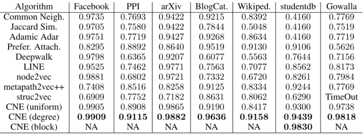
Table 2: The AUC scores for link prediction. TimeOut means aborted after 24 hours. Algorithm Facebook PPI arXiv BlogCat. Wikiped. studentdb Gowalla Common Neigh. 0.9735 0.7693 0.9422 0.9215 0.8392 0.4160 0.7769 Jaccard Sim. 0.9705 0.7580 0.9422 0.7844 0.5048 0.4160 0.7519 Adamic Adar 0.9751 0.7719 0.9427 0.9268 0.8634 0.4160 0.7719 Prefer. Attach. 0.8295 0.8892 0.8640 0.9519 0.9130 0.9106 0.5626 Deepwalk 0.9798 0.6365 0.9207 0.6077 0.5563 0.7644 0.7156 LINE 0.9525 0.7462 0.9771 0.7563 0.7077 0.8562 0.8173 node2vec 0.9881 0.6802 0.9721 0.7332 0.6720 0.8261 0.7984 metapath2vec++ 0.7408 0.8516 0.8258 0.9125 0.8334 0.9244 0.7769 struc2vec 0.6909 0.7752 0.7182 0.8631 0.8062 0.6290 TimeOut CNE (uniform) 0.9905 0.8908 0.9865 0.9190 0.8417 0.9300 0.9738 CNE (degree) 0.9909 0.9115 0.9882 0.9636 0.9158 0.9439 0.9818 CNE (block) NA NA NA NA NA 0.9830 NA 3.2 LINK PREDICTION

In link prediction, we randomly remove50%of the links of the network while keeping it connected. The remaining network is thus used for training the embedding, while the removed links (positive links, labeled1) are used as a part of the test set. Then, the test set is topped up by an equal number

of negative links (labeled0) randomly drawn from the original network. In each repetition of the

experiment, the node indices are shuffled so as to obtain different train-test splits.

We compare CNE with other methods based on the area under the ROC curve (AUC). The methods are evaluated against all datasets mentioned in the previous section. CNE typically works well with small dimensionalitydand sample sizek. In this experiment we setd= 8andk= 50. Only for the two largest networks (arXiv and Gowalla), we increase the dimensionality to d= 16to reduce

underfitting. To calculate AUC, we first compute the posteriorP(aij = 1|Xtrain)of the test links

based on the embeddingXtrainlearned on the training network. Then the AUC score is computed by

comparing the posterior probability of the test links and their true labels.

In this task we first compare CNE against four simple baselines (Grover & Leskovec, 2016): Common Neighbors (|N(i) _∩ N(j)_|), Jaccard Similarity (|N(i)∩N(j)|

|N(i)∪N(j)|), Adamic-Adar Score (P_{t∈N(i)∩N(j)} 1

log|N(t)|), and Preferential Attachment (|N(i)| · |N(j)|). These baselines are neigh-borhood based node similarity measures. We first compute pairwise similarity on the training network. Then from the computed similarities we obtain scores for testing links as the similarity between the two ending nodes. Those scores are then used to compute the AUC against the true labels.

For the NE baselines, we perform link prediction using logistic regression based on the link repre-sentation derived from the node embeddingXtrain. The link representation is computed by applying

the Hadamard operator (element wise multiplication) on the node representationxiandxj, which

is reported to give good results (Grover & Leskovec, 2016). Then the AUC score is computed by comparing the link probability (from logistic regression) of the test links with their true labels.

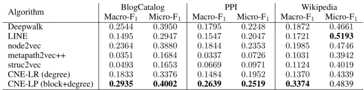
Table 3: The F1scores for multi-label classification.

Algorithm _Macro-F1BlogCatalog_{Micro-F1 Macro-F1}PPI_{Micro-F1 Macro-F1}Wikipedia_Micro-F1 Deepwalk 0.2544 0.3950 0.1795 0.2248 0.1872 0.4661 LINE 0.1495 0.2947 0.1547 0.2047 0.1721 0.5193 node2vec 0.2364 0.3880 0.1844 0.2353 0.1985 0.4746 metapath2vec++ 0.0351 0.1684 0.0337 0.0726 0.1031 0.3942 struc2vec 0.0493 0.1653 0.0669 0.0971 0.1124 0.4019 CNE-LR (degree) 0.1833 0.3376 0.1484 0.1952 0.1370 0.4339 CNE-LP (block+degree) 0.2935 0.4002 0.2639 0.2519 0.3374 0.4839

Results The link prediction results are shown in Table 2. Even with a uniform prior (i.e. prior knowledge only on the overall density), CNE performs better than all baselines on 5 of the 7 networks. With a degree prior, however, CNE outperforms all baselines on all networks. We attribute this to the fact that the degree prior encodes information which is hard to encode using a metric embedding alone. For the multi-relational dataset studentdb, metapath2vec++, which is designed for heterogeneous data, outperforms other baselines but not CNE (regardless of the prior information). Moreover, CNE is capable of encoding the knowledge of the block structure of this multi-relational network as a prior, with each block corresponding to one node type. Doing this improves the AUC further by3.91%

versus CNE with degree prior (from94.39%to98.30%; i.e., a70%reduction in error).

In terms of runtime, over the seven datasets CNE is fastest in two cases, 12% slower than the fastest (metapath2vec++) in one case, and takes approximately twice as long in the four other cases (also metapath2vec++). Detailed runtime results can be found in the supplementary material.

3.3 MULTI-LABEL CLASSIFICATION

We performed multi-label classification on the following networks: BlogCatalog, PPI, and Wikipedia. Detailed results are given in the supplement, while Table 3 contains an excerpt of the results. All baselines are evaluated in a standard logistic regression (LR) setup (Perozzi et al., 2014).

When using logistic regression also on the CNE embeddings, CNE performs on-par, but not particu-larly well (row CNE-LR). This should not be a surprise though, as potentially relevant information encoded by the prior (the degrees) will not be reflected in the embedding. However, multi-label classification can easily be cast as a link prediction problem, by adding to the network a node for each label, with a link to each node to which the label applies. Predicting a label for a node then amounts to predicting a link to that label node. To evaluate this strategy, we train an embedding on the original network plus half the label links, while the other half of the label links is held out for testing. For the baselines, this link prediction setup does not lead to consistent improvements (see supplement), but for CNE it does (row CNE-LP, where LP stands for Link Prediction, in Table 3). On Micro-F1 it is best or once close second best (after LINE with LR, see Table 3), and on Macro-F1it greatly outperforms any other method, suggesting improved performance mainly on the less frequent labels. 3.4 VISUAL EXPLORATION OF MULTI-RELATIONAL DATA

Here we qualitatively evaluate CNE’s ability to facilitate visual exploration of multi-relational data, and how a suitable choice of the prior can help with this. To this end, we use CNE to embed the studentdb dataset directly into 2-dimensional space. As a largerσ2in general appears to give better visual separation between node clusters, we setσ2= 15.

For comparison, we first apply CNE with uniform prior (overall network density). The resulting embedding (Fig. 1a) clearly separates bachelor student/courses/program nodes (upper) from the master’s nodes (lower). Also observe that the embedding is strongly affected by the node degrees (coded as marker size = log degree): high degree nodes flock together in the center. E.g., these are students who interact with many other smaller degree nodes (courses/programs). Although there are no direct links between program nodes (green) and course nodes (blue), the students (red) that connect them are pulling courses towards the corresponding program and pushing away other courses.

(a) contracts profs rooms students tracks courses programs (b) Master Program: Database Bachelor Program Master Program: Computer Networks Master Program: Software Engineering Computer Networks Computer Graphics Software Re-engineering Project: Database _Software Testing Mobile and Wireless network Database Security Seminar: Computer Network Bachelor Program Master Program: Database Master Program:

Computer Networks Master Program:

Software Engineering Prof. #13 Prof. #19 Prof. #13 Prof. #19 Calculus

Figure 1: (a) 2-d embedding with uniform prior. (b) 2-d embedding with degree prior.

Next, we encode the individual node degrees as prior. As in this case the degree information is known, the embedding in addition shows the courses grouped around different programs, e.g.: “Bachelor Program” is close to course “Calculus”; “Master Program Computer Network” is close to course “Seminar Computer Network”; “Master Program Database” is close to course “Database Security”; “Master Program Software Engineering” is close to courses “Software Testing”.

Thus, although this last evaluation remains qualitative and preliminary, it confirms that CNE with a suitable prior can create embeddings that clearly convey information in addition to the given prior.

4 R

W

NE methods typically have three components (Hamilton et al., 2017): (1) A similarity measure between nodes, (2) A metric in embedding space, (3) A loss function comparing proximity between nodes in embedding space with the similarity in the network. Early NE methods such as Laplacian Eigenmaps (Belkin & Niyogi, 2002), Graph factorization (Ahmed et al., 2013), GraRep (Cao et al., 2015), and HOPE (Ou et al., 2016) optimize mean-squared-error loss between Euclidean distance or inner product based proximity and link based (adjacency matrix) similarity in the network. Recently, a few NE methods define node similarity based on paths. Those paths are generated using either the adjacency matrix (LINE, Tang et al., 2015) or random walks (Deepwalk, Perozzi et al. 2014, node2vec, Grover & Leskovec 2016, methapath2vec++, Dong et al. 2017, and struc2vec Ribeiro et al. 2017). Path based embedding methods typically use inner products as proximity measure in the embedding space and optimize a cross-entropy loss. The recent struc2vec method (Ribeiro et al., 2017) uses a node similarity measure that explicitly builds on structural network properties. CNE, unlike the aforementioned methods, unifies the proximity in embeddings space and node similarity using a probabilistic measure. This allows CNE to find a more informative ML embedding.

The question of how to visualize networks on digital screens has been studied for a long time. Recently there has been an uplift in methods to embed networks in a ‘small’ number of dimensions, where small means small as compared to the number of nodes, yet typically much larger than two. These methods enable most machine learning methods to readily apply to tasks on networks, such as node classification or network partitioning. Popular methods include node2vec (Grover & Leskovec, 2016), where for example the default output dimensionality is 128. It is not designed for direct use in visualization, and typically one would fit a higher-dimensional embedding and then apply dimensionality reduction, such as PCA (Peason, 1901) or t-SNE (Maaten & Hinton, 2008) to visualize the data. CNE finds meaningful 2-d embeddings that can be visualized directly. Besides, CNE gives a visualization that conveys maximum information in addition to prior knowledge about the network.

5 C

The literature on NE has so far considered embeddings as tools that are used on their own. Yet, Euclidean embeddings are unable to accurately reflect certain kinds of network topologies, such that

this approach is inevitably limited. We proposed the notion of Conditional Network Embeddings (CNEs), which seeks an embedding of a network that maximally adds information with respect to certain given prior knowledge about the network. This prior knowledge can encode information about the network that cannot be represented well by means of an embedding.

We implemented this conceptually novel idea in a new algorithm based on a simple probabilistic model for the joint of the data and the network, which scales similarly to state-of-the-art NE approaches. The empirical evaluation of this algorithm confirms our intuition that the combination of structural prior knowledge and a Euclidean embedding is extremely powerful. This is confirmed empirically for both the tasks of link prediction and multi-label classification, where CNE outperforms a range of state-of-the-art baselines on a wide range of networks.

In our future work we intend to investigate other models implementing the idea of conditional NEs, alternative and more scalable optimization strategies, as well as the use of other types of structural information as prior knowledge on the network.

ACKNOWLEDGMENTS

The research leading to these results has received funding from the European Research Council under the European Union’s Seventh Framework Programme (FP7/2007-2013) / ERC Grant Agreement no. 615517, from the FWO (project no. G091017N, G0F9816N), and from the European Union’s Horizon 2020 research and innovation programme and the FWO under the Marie Sklodowska-Curie Grant Agreement no. 665501.

R

Florian Adriaens, Jefrey Lijffijt, and Tijl De Bie. Subjectively interesting connecting trees. InJoint European Conference on Machine Learning and Knowledge Discovery in Databases, pp. 53–69. Springer, 2017.

Amr Ahmed, Nino Shervashidze, Shravan Narayanamurthy, Vanja Josifovski, and Alexander J Smola. Distributed large-scale natural graph factorization. In Proceedings of the 22nd international conference on World Wide Web, pp. 37–48. ACM, 2013.

Mikhail Belkin and Partha Niyogi. Laplacian eigenmaps and spectral techniques for embedding and clustering. InAdvances in neural information processing systems, pp. 585–591, 2002.

Bobby-Joe Breitkreutz, Chris Stark, Teresa Reguly, Lorrie Boucher, Ashton Breitkreutz, Michael Livstone, Rose Oughtred, Daniel H Lackner, J¨urg B¨ahler, Valerie Wood, et al. The biogrid interaction database: 2008 update.Nucleic acids research, 36:D637–D640, 2007.

Shaosheng Cao, Wei Lu, and Qiongkai Xu. Grarep: Learning graph representations with global structural information. InProceedings of the 24th ACM International on Conference on Information and Knowledge Management, pp. 891–900. ACM, 2015.

Eunjoon Cho, Seth A Myers, and Jure Leskovec. Friendship and mobility: user movement in location-based social networks. InProceedings of the 17th ACM SIGKDD international conference on Knowledge discovery and data mining, pp. 1082–1090. ACM, 2011.

Yuxiao Dong, Nitesh V Chawla, and Ananthram Swami. metapath2vec: Scalable representation learning for heterogeneous networks. InProceedings of the 23rd ACM SIGKDD International Conference on Knowledge Discovery and Data Mining, pp. 135–144. ACM, 2017.

Bart Goethals, Wim Le Page, and Michael Mampaey. Mining interesting sets and rules in relational databases. InProceedings of the 2010 ACM Symposium on Applied Computing, SAC ’10, pp. 997–1001, New York, NY, USA, 2010. ACM. ISBN 978-1-60558-639-7. doi: 10.1145/1774088. 1774299. URLhttp://doi.acm.org/10.1145/1774088.1774299.

Aditya Grover and Jure Leskovec. node2vec: Scalable feature learning for networks. InProceedings of the 22nd ACM SIGKDD international conference on Knowledge discovery and data mining, pp. 855–864. ACM, 2016.

William L Hamilton, Rex Ying, and Jure Leskovec. Representation learning on graphs: Methods and applications.arXiv preprint arXiv:1709.05584, 2017.

FC Leone, LS Nelson, and RB Nottingham. The folded normal distribution. Technometrics, 3(4): 543–550, 1961.

Jure Leskovec and Andrej Krevl. SNAP Datasets: Stanford large network dataset collection, 2015. Laurens van der Maaten and Geoffrey Hinton. Visualizing data using t-SNE. Journal of machine

learning research, 9(Nov):2579–2605, 2008.

Matt Mahoney. Large text compression benchmark. URL: http://www. mattmahoney. net/text/text. html, 2011.

Mingdong Ou, Peng Cui, Jian Pei, Ziwei Zhang, and Wenwu Zhu. Asymmetric transitivity preserv-ing graph embeddpreserv-ing. InProceedings of the 22nd ACM SIGKDD international conference on Knowledge discovery and data mining, pp. 1105–1114. ACM, 2016.

K Peason. On lines and planes of closest fit to systems of point in space.Philosophical Magazine, 2 (11):559–572, 1901.

Bryan Perozzi, Rami Al-Rfou, and Steven Skiena. Deepwalk: Online learning of social representa-tions. InProceedings of the 20th ACM SIGKDD international conference on Knowledge discovery and data mining, pp. 701–710. ACM, 2014.

Leonardo FR Ribeiro, Pedro HP Saverese, and Daniel R Figueiredo. struc2vec: Learning node representations from structural identity. InProceedings of the 23rd ACM SIGKDD International Conference on Knowledge Discovery and Data Mining, pp. 385–394. ACM, 2017.

Jian Tang, Meng Qu, Mingzhe Wang, Ming Zhang, Jun Yan, and Qiaozhu Mei. Line: Large-scale information network embedding. InProceedings of the 24th International Conference on World Wide Web, pp. 1067–1077. International World Wide Web Conferences Steering Committee, 2015. Matthijs van Leeuwen, Tijl De Bie, Eirini Spyropoulou, and C´edric Mesnage. Subjective

interesting-ness of subgraph patterns. Machine Learning, 105(1):41–75, 2016. Reza Zafarani and Huan Liu. Social computing data repository at asu, 2009.

CONDITIONAL

NETWORK

EMBEDDINGS:

SUPPLE

-MENT

Bo Kang, Jefrey Lijffijt & Tijl De Bie

Department of Electronics and Information Systems (ELIS), IDLab Ghent University

Ghent, Belgium

{firstname.lastname_}@ugent.be

1 D

Denote the Euclidean distance between two points asdij ,||xi−xj||2. The derivative ofdijwith

respect to embeddingxiof nodeireads:

∇xidij= xi−xj

dij

Then the derivative of the log posterior with respect toxiis given by:

∇xilog (P(G|X)) = X j:{i,j}∈E _{∂log (P(G} |X)) ∂dij + ∂log (P(G_|X)) ∂dji ∇xidij + X j:{i,j}∈/E _{∂log (P(G} |X)) ∂dij +∂log (P(G|X)) ∂dji ∇xidij = 2 X j:{i,j}∈E ∂log (P(G|X)) ∂dij xi−xj dij + 2 X j:{i,j}∈/E ∂log (P(G|X)) ∂dij xi−xj dij

Using shorthand notation_Nij,σ1 =N+ dij|σ

2 1 and_Nij,σ2 =N+ dij|σ 2 2

, we can compute the partial derivative ∂log(P(G|X))

∂dij for{i, j} ∈Eas: ∂log (P(G|X)) ∂dij = ∂ ∂dij X {i,j}∈E

log (Nij,σ1Pij)−log (Nij,σ1Pij+Nij,σ2(1−Pij))

=Nij,σ1Pij· −dij σ2 1 Nij,σ1Pij −Nij,σ1Pij· −dij σ2 1 +Nij,σ2(1−Pij)· −dij σ2 2 Nij,σ1Pij+Nij,σ2(1−Pij) =₋dij σ2 1 +P(aij= 1|X) dij σ2 1 +P(aij = 0|X) dij σ2 2 Similarly, the partial derivative∂log(P(G|X))

∂dij for{i, j}∈/Ereads: ∂log (P(G|X)) ∂dij =₋dij σ2 2 +P(aij = 1|X) dij σ2 1 +P(aij= 0|X) dij σ2 2 . The partial derivatives ∂Nmn,σPmn

∂dij are nonzero only whenm=iandn=j, which gives the final

gradient: ∇xilog (P(G|X)) = 2 X j:{i,j}∈E (xi−xj)P(aij= 0|X) ₁ σ2 2 − 1 σ2 1 + 2 X j:{i,j}∈/E (xi−xj)P(aij = 1|X) ₁ σ2 1 − 1 σ2 2 (1)

-10 -8 -6 -4 -2 0 2 4 6 8 10 0 0.1 0.2 0.3 0.4 0.5 0.6 0.7 0.8 0.9 1 a ij = 1 ( p=0.1, 2=2 ) a ij = 0 (p=0.1, 2=2) a_ij = 1 (p=0.1, ₂=10) a ij = 0 (p=0.1, 2=10) -10 -8 -6 -4 -2 0 2 4 6 8 10 0 0.1 0.2 0.3 0.4 0.5 0.6 0.7 0.8 0.9 1 a ij = 1 ( p=0.9, 2=2 ) a ij = 0 (p=0.9, 2=2) a_ij = 1 (p=0.9, ₂=10) a ij = 0 (p=0.9, 2=10)

Figure 1: The posterior distributionP(aij = 1|X)andP(aij= 0|X)with different prior probability

Pij andσ2

2 D

P

(

G

_|

X

)

logP(G_|X) = log   Y {i,j}∈E Nij,σ1Pij Nij,σ1Pij+Nij,σ2(1−Pij) · Y {k,l}∈/E Nkl,σ2(1−Pkl) Nkl,σ1Pkl+Nkl,σ2(1−Pkl)   = log   Y {i,j}∈E 1 1 + Nij,σ₂(1−Pij) Nij,σ1Pij · Y {k,l}∈/E 1 1 + Nkl,σ1Pkl Nkl,σ₂(1−Pkl)   =− X {i,j}∈E log 1 + (2πσ 2 2)−1/2exp −d2ij/(2σ22) (1−Pij) (2πσ2 1)−1/2exp −d2ij/(2σ12) Pij ! − X {k,l}∈/E log 1 + (2πσ 2 1)−1/2exp −d2kl/(2σ21) Pkl (2πσ2 2)−1/2exp (−dkl2/(2σ22)) (1−Pkl) ! =₋ X {i,j}∈E log 1 + σ1 σ2 1₋Pij Pij exp 1 σ2 1 − 1 σ2 2 _d2 ij 2 !! − X {k,l}∈/E log 1 + σ2 σ1 Pkl 1₋Pkl exp ₁ σ2 2 − 1 σ2 1 _d2 kl 2 (2)

3 E

σ

σ

CNE seeks the embeddingXthat maximizes the likelihoodP(G_|X)for givenG. To understand the effect of parameterσ1andσ2we plot the posteriorP(aij = 1|X)as well asP(aij = 0|X)in

Figure 1. The plot shows a largeσ2corresponds to more extreme minima of the objective function (Fig1a), thus results in stronger push and pulling effect in the optimization. Large link probability in the network prior further strengthen the pushing and pulling effects (Fig 1b). The flat area in Figure 1b (σ2= 10) allows connected nodes to keep some small distance from each other, and larger σ2also allows larger corrections to the prior probabilities (both Fig 1a and Fig 1b), but also makes the optimization problem harder.

4 B

• Deepwalk (Perozzi et al., 2014): This embedding algorithm learns embedding based on the similarities between nodes. The proximities are measured by random walks. The transition probability of walking from one node to all its neighbors are the same and are based on one-hop connectivity.

• LINE (Tang et al., 2015): Instead of random walks, this algorithm defines similarity between nodes based on first and second order adjacencies of the given network.

• node2vec (Grover & Leskovec, 2016): This is again based on random walks. In addition to its predecessors, it offers two parametersp,qthat interpolates the importance of BFS and DFS like random walk in the learning.

• metapath2vec++ (Dong et al., 2017): This approach is developed for heterogeneous NE, namely, the nodes belong to different node types. methapath2vec++ performs random walks by hopping from a node form one type to a node from another type. It also utilizes the node type information in the softmax based objective function.

• struc2vec (Ribeiro et al., 2017): The method first measures the structural information by computing pairwise similarity between nodes using a range of neighborhood sizes. This results in a multilayer weighted graph where the edge weights on the same layer are derived from the node similarity computed on one neighborhood size. Then the embedding is constructed by a random walk strategy that navigates the multilayer graph.

5 N

We used the following commonly used benchmark networks in the experiments:

• Facebook (Leskovec & Krevl, 2015): In this network, nodes are the users and links represent the friendships between the users. The network has 4,039 nodes and 88,234 links.

• arXiv ASTRO-PH (Leskovec & Krevl, 2015): In this network nodes represent authors of papers submitted to arXiv. The links represents the collaborations: two authors are connected if they co-authored at least one paper. The network has 18,722 nodes and 198,110 links.

• studentdb (Goethals et al., 2010): This is a snapshot of the student database from the University of Antwerp’s Computer Science department. There are 403 nodes that belong to one of the following node types including: course, student, professor, program, track, contract, and room. There 3429 links that are the binary relationships between the nodes: student-in-track, student-in-program, student-in-contract, student-take-course, professor-teach-course, course-in-room. The database schema is given in Figure 2.

• Gowalla (Cho et al., 2011): This is a undirected location-based friendship network. The network has 196,591 nodes, 950,327 links.

• BlogCatalog (Zafarani & Liu, 2009): This social network contains nodes representing bloggers and links representing their relations with other bloggers. The labels are the bloggers’ interests inferred from the meta data. The network has 10,312 nodes, 333,983 links, and 39 labels (used for multi-label classifications).

• Protein-Protein Interactions (PPI) (Breitkreutz et al., 2007): A subnetwork of the PPI network for Homo Sapiens. The subnetwork has 3,890 nodes, 76,584 links, and 50 labels. • Wikipedia (Mahoney, 2011): This network contains nodes representing words and links representing the co-occurrence of words in Wikipedia pages. The labels represents the inferred Part-of-Speech tags (Toutanova et al., 2003). The network has 4,777 nodes, 184,812 links, and 40 different labels.

6 D

-

In the multi-label classification setting, each node is assigned one or more labels. For training,50%

of the nodes and all their labels are used for training. The labels of the remaining nodes need to be predicted. We train CNE and baselines based on the full network. Then50%of the nodes are randomly selected to train a L2 regularized logistic regression classifier. The regularization strength

Track Program Contract Student Professor Course Room 1:N N:1 M:N M:N 1:N 1:N

Figure 2: The entity relationship diagram of the studentdb dataset.

parameter of the classifier is trained with 10-fold cross-validation (CV) on the training data. We report the Macro-F1and Micro-F1based on the predictions. For the logistic regression classifier (sklearn, Pedregosa et al., 2011) we require every fold to have at least one positive and one negative label and we removed the labels that occur fewer than10times (number of folds in CV) in the data.

The detailed results of this approach based on logistic regression are shown in the upper half of Table 1. For CNE (written as CNE-LR to emphasize logistic regression was used for classifying), the embeddings are obtained withd= 32andk= 150(without optimizing). Somewhat surprisingly, CNE still performs in line with the state-of-the-art graph embedded methods, although without improving on them (on BlogCatalog, CNE performs third out of five methods, in PPI and Wikipedia it performs fourth out of five). This is surprising, given the fact that CNE yields embeddings that, by design, do not reflect certain information about the nodes that may be useful in classifying (here, their degree).

Multi-label classification can however be cast as a link prediction problem—a task we know CNE performs well at. To do this, we insert a node into the network corresponding to each of labels, and link the original nodes to the label nodes if they have that label. We can then employ link prediction, exactly as in the link prediction case (training on the full network, but with only50%of the edges between original nodes and label nodes, and the other half for testing), to do multi-label classification. For CNE, besides a degree prior, we can encode a ’block’ prior which encodes the average connectivity between original nodes–original nodes, original nodes–labels, and labels–labels (which is zero, as labels are not connected to each other). Note that this approach means that also neighborhood-based link prediction methods can be used for multi-label classification.

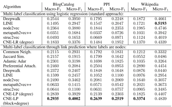
The detailed results of this link prediction approach to multi-label classification are shown in the lower half of Table 1. CNE-LP (block+degree) (with LP to indicate it is based on link prediction) consistently outperforms all baselines on Macro-F1, while on Micro-F1it is best on two datasets (BlogCatalog and PPI), and close second-best on one (Wikipedia). We note that while the benefit of this link prediction approach to multi-label classification is clear (and unsurprising) for CNE, there is no consistent benefit to other methods. This shows that the superior performance of CNE-LP for multi-label classification is not (or at least not exclusively) thanks to the link prediction approach, but at least in part also thanks to a more informative embedding when considered in combination with the prior.

7 R

We compare the runtime (in second) of CNE with other baselines in this section. We use the parameters settings in link prediction task for all methods. Namely, for CNE, we setd= 8(For arXiv

k= 16to reduce underfitting) andk= 50. We set stopping criterion of CNE||∇X||∞<10−2or

maxIter <250(whichever is met first). These stopping criteria yield embeddings with the same

performance in link prediction tasks as reported in the paper. For other methods, we use the default setting as reported in their original paper. The hyper-parametersp,qof node2vec are tuned using

Table 1: The F1scores for multi-label classification.

Algorithm _Macro-F1BlogCatalog_{Micro-F1 Macro-F1}PPI_{Micro-F1 Macro-F1}Wikipedia_Micro-F1 Multi-label classification using logistic regression (standard approach):

Deepwalk 0.2544 0.3950 0.1795 0.2248 0.1872 0.4661 LINE 0.1495 0.2947 0.1547 0.2047 0.1721 0.5193 node2vec 0.2364 0.3880 0.1844 0.2353 0.1985 0.4746 metapath2vec++ 0.0351 0.1684 0.0337 0.0726 0.1031 0.3942 struc2vec 0.0493 0.1653 0.0669 0.0971 0.1124 0.4019 CNE-LR (degree) 0.1833 0.3376 0.1484 0.1952 0.1370 0.4339

Multi-label classification through link prediction where labels are nodes:

Common Neigh. 0.2115 0.2931 0.1792 0.1831 0.1212 0.3332 Jaccard Sim. 0.2157 0.1915 0.1799 0.1642 0.0552 0.0486 Adamic Adar 0.2301 0.3198 0.1698 0.1825 0.1035 0.3264 Preferential Attach. 0.2460 0.2084 0.2504 0.0953 0.2890 0.4454 Deepwalk 0.2372 0.2407 0.1848 0.1648 0.0876 0.0440 LINE 0.1599 0.2457 0.1052 0.1100 0.0976 0.2954 node2vec 0.2490 0.3462 0.2081 0.2069 0.1640 0.3057 metapath2vec++ 0.0633 0.1415 0.0571 0.0542 0.2021 0.3673 struc2vec 0.0644 0.1100 0.0631 0.0757 0.0905 0.3485 CNE-LP (degree) 0.2839 0.3929 0.2139 0.2303 0.1825 0.4407 CNE-LP (block+degree) 0.2935 0.4002 0.2639 0.2519 0.3374 0.4839

Table 2: The runtime (in seconds) of embedding methods. TimeOut means aborted after 24 hours. Algorithm Facebook PPI arXiv BlogCat. Wikiped. studentdb Gowalla Deepwalk 120.78 116.09 714.68 344.72 138.89 8.34 5717.67 LINE 253.20 203.92 649.98 218.20 232.11 180.35 10988.71 node2vec 86.61 64.96 291.42 1054.73 288.32 6.04 5593.52 metapath2vec++ 130.78 39.59 274.60 332.19 78.14 3.50 333.29 struc2vec 2692.96 1105.41 54218.82 1356.67 1691.79 9245.23 TimeOut CNE (uniform) 86.89 75.15 728.74 227.11 92.35 7.25 642.14 CNE (degree) 77.80 70.35 579.85 204.48 87.69 6.80 670.26 CNE (block) NA NA NA NA NA 10.68 NA

cross validation. This experiment is performed with single process/thread on a desktop with CPU 2,7 GHz Intel Core i5 and RAM 16 GB 1600 MHz DDR3. Table 2 summarizes the runtime of all methods against all datasets we used in the paper. Over the seven datasets CNE is fastest in two cases, 12% slower than the fastest in one case (metapath2vec++), and approximately twice slower in the four other cases (also metapath2vec++).

R

Bobby-Joe Breitkreutz, Chris Stark, Teresa Reguly, Lorrie Boucher, Ashton Breitkreutz, Michael Livstone, Rose Oughtred, Daniel H Lackner, J¨urg B¨ahler, Valerie Wood, et al. The biogrid interaction database: 2008 update.Nucleic acids research, 36:D637–D640, 2007.

Eunjoon Cho, Seth A Myers, and Jure Leskovec. Friendship and mobility: user movement in location-based social networks. InProceedings of the 17th ACM SIGKDD international conference on Knowledge discovery and data mining, pp. 1082–1090. ACM, 2011.

Yuxiao Dong, Nitesh V Chawla, and Ananthram Swami. metapath2vec: Scalable representation learning for heterogeneous networks. InProceedings of the 23rd ACM SIGKDD International Conference on Knowledge Discovery and Data Mining, pp. 135–144. ACM, 2017.

Bart Goethals, Wim Le Page, and Michael Mampaey. Mining interesting sets and rules in relational databases. InProceedings of the 2010 ACM Symposium on Applied Computing, SAC ’10, pp. 997–1001, New York, NY, USA, 2010. ACM. ISBN 978-1-60558-639-7. doi: 10.1145/1774088. 1774299. URLhttp://doi.acm.org/10.1145/1774088.1774299.

Aditya Grover and Jure Leskovec. node2vec: Scalable feature learning for networks. InProceedings of the 22nd ACM SIGKDD international conference on Knowledge discovery and data mining, pp. 855–864. ACM, 2016.

Jure Leskovec and Andrej Krevl. SNAP Datasets: Stanford large network dataset collection, 2015. Matt Mahoney. Large text compression benchmark. URL: http://www. mattmahoney. net/text/text.

html, 2011.

Fabian Pedregosa, Ga¨el Varoquaux, Alexandre Gramfort, Vincent Michel, Bertrand Thirion, Olivier Grisel, Mathieu Blondel, Peter Prettenhofer, Ron Weiss, Vincent Dubourg, et al. Scikit-learn: Machine learning in python.Journal of machine learning research, 12(Oct):2825–2830, 2011. Bryan Perozzi, Rami Al-Rfou, and Steven Skiena. Deepwalk: Online learning of social

representa-tions. InProceedings of the 20th ACM SIGKDD international conference on Knowledge discovery and data mining, pp. 701–710. ACM, 2014.

Leonardo FR Ribeiro, Pedro HP Saverese, and Daniel R Figueiredo. struc2vec: Learning node representations from structural identity. InProceedings of the 23rd ACM SIGKDD International Conference on Knowledge Discovery and Data Mining, pp. 385–394. ACM, 2017.

Jian Tang, Meng Qu, Mingzhe Wang, Ming Zhang, Jun Yan, and Qiaozhu Mei. Line: Large-scale information network embedding. InProceedings of the 24th International Conference on World Wide Web, pp. 1067–1077. International World Wide Web Conferences Steering Committee, 2015. Kristina Toutanova, Dan Klein, Christopher D Manning, and Yoram Singer. Feature-rich part-of-speech tagging with a cyclic dependency network. InProceedings of the 2003 Conference of the North American Chapter of the Association for Computational Linguistics on Human Language Technology-Volume 1, pp. 173–180. Association for Computational Linguistics, 2003.