High order second derivative methods with Runge--Kutta stability for the numerical solution of stiff ODEs

Vol. 5, No. 2, (2015), pp 1-10

High order second derivative methods

with Runge–Kutta stability for the

numerical solution of stiff ODEs

A. Abdi∗ and G. Hojjati

Abstract

We describe the construction of second derivative general linear methods (SGLMs) of orders five and six. We will aim for methods which areA–stable and have Runge–Kutta stability property. Some numerical results are given to show the efficiency of the constructed methods in solving stiff initial value problems.

Keywords: Ordinary differential equation; General linear methods; Runge– Kutta stability; A–stability; Second derivative methods.

1 Introduction

In many fields such as control theory, chemical kinetics, biology and the movement of stars in galaxies, dynamic behavior is modeled by systems of ordinary differential equations (ODEs). We consider the autonomous ODEs in the form

y′(x) =f(y(x)), x∈[x0, x],

y(x0) =y0,

(1)

wheref :Rm→Rmandm is the dimensionality of the system. We restrict our attention to autonomous systems because non-autonomous systems can be made autonomous by adding an extra equation to the system.

For system (1), let g := fyf. For problems in which g can be

calcu-lated along with f, at a moderate additional cost, second derivative meth-ods become feasible. General linear methmeth-ods (GLMs) [6, 7, 12] as a unifying

∗_{Corresponding author}

Received 15 October 2014; revised 15 February 2015; accepted 21 February 2015 A. Abdi

Faculty of Mathematical Sciences, University of Tabriz, Tabriz, Iran. e-mail: a [email protected]

G. Hojjati

Faculty of Mathematical Sciences, University of Tabriz, Tabriz, Iran. email: [email protected]

2 A. Abdi and G. Hojjati framework for the traditional methods, like Runge–Kutta methods, linear multistep methods, predictor–corrector methods and hybrid methods, have been extended to the second derivative general linear methods (SGLMs) by Butcher and Hojjati [8]. These methods which are s-stage and r-value, for the numerical solution of (1) are given by

Y[n] =h(A⊗Im)F(Y[n]) +h2(A⊗Im)G(Y[n]) + (U⊗Im)y[n−1],

y[n] =h(B⊗Im)F(Y[n]) +h2(B⊗Im)G(Y[n]) + (V ⊗Im)y[n−1],

(2)

where h is the stepsize, A, A ∈ Rs×s, U ∈ Rs×r, B, B ∈ Rr×s and V ∈

Rr_×r _{and notation⊗is the Kronecker product. Here, Y}[n] _{= [Y}[n]

i ] s

i=1 is an

approximation of stage orderqto the vectory(xn−1+ch) = [y(xn−1+cih)]si=1,

i.e.

Y_i[n]=

q ∑

k=0

ck i

k!h

k

y(k)(xn−1) +O(hq+1), i= 1,2, . . . , s, (3)

F(Y[n]_{) := [f(Y}[n]

i )]si=1 and G(Y[n]) := [g(Y [n]

i )]si=1 where the vector c =

[c1 c2 · · · cs]T is the abscissa vector. Also the vectors y[n−1] = [y

[n−1]

i ]

r i=1

and y[n] = [y_i[n]]r_i=1 are the input and output vectors at the step numbern, respectively, which for a method of orderptake the following forms

y_i[n−1]=

p ∑

k=0

αikhky(k)(xn−1) +O(hp+1), i= 1,2, . . . , r, (4)

and

y_i[n] =

p ∑

k=0

αikhky(k)(xn) +O(hp+1), i= 1,2, . . . , r, (5)

for someαik∈Rassociated with the method.

The main features of SGLMs including pre-consistency, consistency, zero-stability and types of these methods have been discussed in [3]. It has been shown in [4] that the SGLM (2) with the input vector (4) has order p and stage order q=piff

ecz =zAecz+z2Aecz+U w(z) +O(zp+1), (6)

ezw(z) =zBecz+z2Becz+V w(z) +O(zp+1). (7)

where

ecz=

[

ec1z _ec2z · · · _ecsz

]T

,

andw(z) is a vector with elements given by

wi(z) = p ∑

k=0

In the special SGLMs with p = q = r = s, U = Is and Ve = e, e =

[1,1, . . . ,1]T _{∈ R}s_{, an equivalent condition for order conditions has been}

found in [5] as

B=B0−AB1−AB2−V B3−(B−V A)B4+V A,

where the (i, j) elements ofB0,B1,B2,B3, andB4are given respectively by

∫1+ci

0 ϕj(x)dx

ϕj(cj)

, ϕj(1 +ci) ϕj(cj)

, ϕ

′

j(1 +ci)

ϕj(cj)

,

∫ci

0 ϕj(x)dx

ϕj(cj)

, ϕ

′

j(ci)

ϕj(cj)

.

Here,

ϕi(x) = s ∏

j=1,j̸=i

(x−cj), i= 1,2,· · · , s.

Construction of SGLMs which are also suitable for the numerical solution of differential algebraic equations (DAEs) has been discussed in [10]. Some ob-tained order barries for different types of SGLMs, found in [3,4,10], are useful in construction of these methods. These barriers have been also confirmed by means of order arrows by Abdi and Butcher [1, 2]. Recently, efficiency of these methods in solving stiff ODEs arising from chemical reactions has been shown in [11].

In continuation of studying on SGLMs, in this paper we construct A– stable methods of orders five and six with r = s = 3 and Runge–Kutta stability property.

Next sections of this paper are organized as follows: In Sec. 2, we discuss about stability behaviour of Runge–Kutta stable three-stage methods. Sec. 3 is devoted to construction of SGLMs of orders five and six withA–stability property. Some numerical experiments are given in Sec. 4 to demonstrate the efficiency of the constructed methods.

2 RKS three-stage methods

We first recall that the stability matrix for SGLMs can be obtained by ap-plying the methods to the standard test problem of Dahlquist [9] y′ = ζy, whereζ is a complex number, which it is

M(z) =V +(zB+z2B)(I−zA−z2A)−1U,

wherez=hζ. Thus, we are interested in stable behavior of powers ofM(z). IfM(z) has only a single non-zero eigenvalue, R(z), then the method is said to possess Runge-Kutta stability (RKS) property. For RKS methods, the stability behaviour is related toR(z).

4 A. Abdi and G. Hojjati with the same elementsλandµon the diagonal, respectively,R(z) takes the form

R(z) = N(z)

(1−λz−µz2₎s, (8)

where deg(N)≤2s. For the methods of order five and six with three stages that will be discussed in Sec. 3, the polynomialN defined in (8) satisfies

N(z) = (1−λz−µz2)3ez−C5z6+O(z7),

and

N(z) = (1−λz−µz2)3ez+O(z7),

respectively, for an arbitraryC5as the error constant of the method. For the

method of order six, the error constant is

C6=

1 5040−

1 240λ−

1 40µ+

1 4λµ+

( 1 40−

1 2µ

)

λ2+(1 2−

3 2λ

)

µ2− 1

24λ

3_−µ3_.

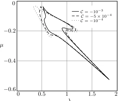
For these methods to be A–stable, using E-polynomial theorem [7], it is necessary and sufficient that λ > 0, µ < 0, and so that the E(y) is non-negative fory real where the E-polynomial is defined by

E(y) =|1−λiy+µy2|6− |N(iy)|2,

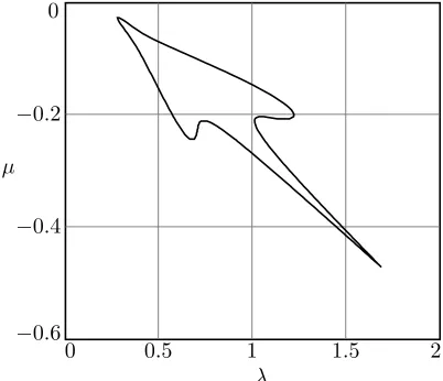
whereiis the imaginary unit. The boundary of the regions ofA-stable choices of (λ, µ) for the methods of order five (with different values ofC5) and order

six are plotted in Figure 1 and Figure 2.

λ µ

0 0.5 1 1.5 2

−0.6 −0.4 −0.2 0

C=−10−3

C=−5×10−4 C=−10−4

λ µ

0 0.5 1 1.5 2

−0.6 −0.4 −0.2 0

Figure 2: The boundary of the region ofA–stable choices of (λ, µ) fors= 3,p= 6

3

A

–stable RKS methods of orders 5 and 6

Construction SGLMs of orders p=q≤4 has been discussed in [3–5, 10]. In this section, we construct A–stable three-stage methods of orders five and six with RKS property. Throughout the construction of these methods, we will consider U =Is and V = evT where v ∈ Rr and vTe = 1. The later

guarantees zero-stability of the methods [3].

3.1 Order 5 methods

6 A. Abdi and G. Hojjati A=    

0.6000000000 0 0

0.4538633794 0.6000000000 0

0.8442059328 0.8999163314 0.6000000000

   , A=    

−0.1000000000 0 0

−0.1450566118−0.1000000000 0 −0.9847293116−0.1278647721−0.1000000000

   , B=    

0.3902646263 0.4639576064 0.2524239604

−0.3312778090 1.1306242731 0.3534363496 5.0478598121−4.1644469839−0.5208888994

   , B=    

−0.2677332867−0.3732899225−0.0223237563 −0.4095181371−0.6362626571−0.0357186615 0.5750983052 1.6053219094 0.0622616286

   ,

v=[1.2203054517−0.3423946125 0.1220891608]T.

This method isA–stable with the error constantC5≈ −3.50×10−4.

3.2 Order 6 methods

Choosingc= [0 c1 1]T,c1as a free parameter, and solving the order

condi-tions and the nonlinear RKS condicondi-tions, we getc1=−1.4989329045 and the

coefficients matrices of the method take the following forms

A=

   

0.4007120047 0 0

0.5574459850 0.4007120047 0

0.7281456081 0.0121320319 0.4007120047

   , A=    

−0.0612701047 0 0

−0.0145743957−0.0612701047 0 0.3881180321 0.1117302066 −0.0612701047

   , B =    

1.1371686053 0.2249968367 0.0903218055

−0.0512895056 0.1078326109−0.6604347472 1.5642870990 0.3929237249−0.2450012162

B=

   

−0.0425486219 0.0078897842−0.0128566928 0.1945434509−0.0296649869 0.0449770864

0.3584398092 0.0701030286−0.0116769898

   ,

v=[0.8572479903 0.2113738061−0.0686217964]T.

The obtained value for (λ, µ) is the interior of the region ofA–stable choices presented in Figure 2. The error constant for thisA–stable method isC6≈

2.56×10−5.

4 Numerical verifications

In this section we present some numerical results by applying the constructed methods of orders five and six in Sec. 3, in order to demonstrate the theo-retical expectations. Computational experiments are carried out by applying the methods to the following two stiff problems.

S1– The non-linear stiff test problem

{

y₁′(x) =−1002y1(x) + 1000y22(x), y1(0) = 1,

y2′(x) =y1(x)−y2(x)(1 +y2(x)), y2(0) = 1.

The exact solution is y1(x) = exp(−2x) and y2(x) = exp(−x) and

x∈[0,1].

S2– The stiff initial value problem arose from a chemistry problem

      

y′₁(x) =−0.013y2−1000y1y2−2500y1y3, y1(0) = 0,

y′₂(x) =−0.013y2−1000y1y2, y2(0) = 1,

y′₃(x) =−2500y1y3, y3(0) = 1.

The reference solution atx= 2 is

y1(2) =−0.3616933169289×10−5,

y2(2) = 0.9815029948230,

y3(2) = 1.018493388244.

Numerical results for the Problem S1, reported in Table 1, illustrate accuracy of the methods of order 5 and 6. These results are obtained with fixed stepsizes h= 1/2k with several integer values for k. In this table, we have listed norm of error ∥eh(x)∥ at the endpoint of integration x = 1. Also,

8 A. Abdi and G. Hojjati convergence, computed by the formula p = log₂(∥eh(x)∥/∥eh/2(x)∥) where

eh(x) andeh/2(x) are errors corresponding to stepsizes handh/2.

Table 1: The global error at the end of the interval of integration [0,1] for problem S1

h 2−2 2−3 2−4 2−5

Order 5 method 2.25×10−7 _5.61×10−9 _1.51×10−10 _4.34×10−12

p 5.33 5.22 5.12

Order 6 method 6.92×10−8 2.94×10−10 2.45×10−12 5.03×10−14

p 7.88 6.91 5.61

Numerical results for the Problem S2 are given in Table 2 with stepsize

h= 0.001. Comparing the obtained results by the methods with the refer-ence solution shows the efficiency of the methods for solving stiff non-linear problems.

Table 2: Numerical results for problem S2 solved by the methods of orders five and six

x y Order 5 method Order 6 method

y1 −0.3616933169478728×10−5 −0.3616933215630078×10−5

2 y2 0.9815029948594308 0.9815030036954803 y3 1.018493388207507 1.018493379371295

0 0.5 1 1.5 2

10−16

10−15

10−14

10−13

10−12

x

2+y

1

−y

2

−y

3

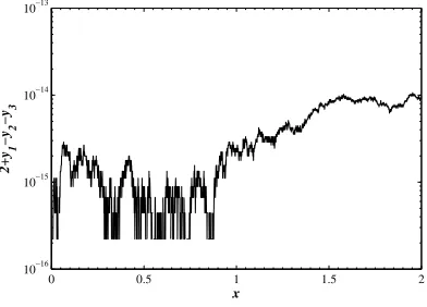
Figure 3: Variation of 2 +y1−y2−y3 versusxwhichy1,y2and y3 are the

0 0.5 1 1.5 2

10−16

10−15

10−14

10−13

x

2+y

1

−y

2

−y

3

Figure 4: Variation of 2 +y1−y2−y3 versusxwhichy1,y2and y3 are the

numerical solutions obtained by the method of order 6

The differential equations in Problem S2 satisfy a linear conservation law

2 +y1(x)−y2(x)−y3(x) = 0, (9)

for allx. In Figure 3 and Figure 4, we have plotted the graph of 2+y1−y2−y3

versusx. We observe that for both methods of orders five and six equation (9) for the obtained numerical solutions holds approximately with high accuracy which demonstrate the accuracy of the applied methods.

5 Conclusion

For methods of higher orders (p≥5) withp=q=r=s, it is no longer pos-sible to solve the nonlinear systems of equations for satisfying RKS property by symbolic manipulation packages [5]. It seems that this difficulty does not appear for methods with fewer stages. In this paper we constructed RKS methods of ordersp= 5 andp= 6 withr=s= 3.

References

1. Abdi, A. and Butcher, J. C. Order bounds for second derivative approci-mations, BIT, 52 (2012) 273–281.

10 A. Abdi and G. Hojjati 3. Abdi, A. and Hojjati, G.An extension of general linear methods, Numer.

Algor., 57 (2011) 149–167.

4. Abdi, A. and Hojjati, G. Maximal order for second derivative general linear methods with Runge–Kutta stability, Appl. Numer. Math., 61 (2011) 1046–1058.

5. Abdi, A., Bra`s, M. and Hojjati, G. On the construction of second derivative diagonally implicit multistage integration methods, Appl. Numer. Math., 76 (2014) 1–18.

6. Butcher, J. C.On the convergence of numerical solutions to ordinary dif-ferential equations, Math. Comp., 20 (1966) 1–10.

7. Butcher, J. C. Numerical Methods for Ordinary Differential Equations, Wiley, New York, 2008.

8. Butcher, J. C. and Hojjati, G.Second derivative methods with RK stability, Numer. Algor., 40 (2005) 415–429.

9. Dahlquist, G.A special stability problem for linear multistep methods, BIT, 3 (1963) 27–43.

10. Ezzeddine, A. K., Hojjati, G. and Abdi, A. Sequential second derivative general linear methods for stiff systems, Bull. Iranian Math. Soc., 40 (2014) 83–100.

11. Hojjati, G., Abdi, A., Mirzaee, F. and Bimesl, S.Numerical solution of stiff systems of differential equations arising from chemical reactions, Iran. J. Numer. Anal. Optim., 4 (2014) 25–39.

ﯽﻟﻮﻤﻌﻣ ﻞﯿﺴﻧاﺮﻔﯾد تﻻدﺎﻌﻣ یدﺪﻋ ﻞﺣ یاﺮﺑ ﺎﺗﻮﮐ-ﮓﻧار یراﺪﯾﺎﭘ ﺎﺑ ﻻﺎﺑ ﻪﺒﺗﺮﻣ مود ﻖﺘﺸﻣ یﺎﻫشور ﺖﺨﺳ

ﯽﺘﺠﺣ ﺎﺿﺮﻣﻼﻏ و یﺪﺒﻋ ﯽﻠﻋ

ﯽﺿﺎﯾر مﻮﻠﻋ هﺪﮑﺸﻧاد ،ﺰﯾﺮﺒﺗ هﺎﮕﺸﻧاد

ﻒﯿﺻﻮﺗ و ﺚﺤﺑ ار ﺶﺷ و ﺞﻨﭘ ﺐﺗاﺮﻣ زا (SGLMs) مود ﻖﺘﺸﻣ ﯽﻣﻮﻤﻋ ﯽﻄﺧ یﺎﻬ-ﺷور ﺖﺧﺎﺳ: هﺪﯿﮑﭼ

ﺎﺗﻮﮐ-ﮓﻧار یراﺪﯾﺎﭘ ﺖﯿﺻﺎﺧ یاراد و هدﻮﺑ راﺪﯾﺎﭘ - A هﺪﺷ ﻪﺘﺧﺎﺳ یﺎﻬ-ﺷور ،ﯽﺳرﺮﺑ ﻦﯾا رد .ﻢﯿﻨﮐ ﯽﻣ ﻪﯿﻟوا راﺪﻘﻣ ﻞﺋﺎﺴﻣ ﻞﺣ یاﺮﺑ هﺪﺷ ﻪﺘﺧﺎﺳ یﺎﻬ-ﺷور ﯽﯾارﺎﮐ نداد نﺎﺸﻧ یاﺮﺑ یدﺪﻋ ﺞﯾﺎﺘﻧ ﯽﺧﺮﺑ .ﺪﻨﺘﺴﻫ . ﺪﻧﻮﺷ ﯽﻣ ﻪﺋارا ﺖﺨﺳ

؛یراﺪﯾﺎﭘ - A ؛ﺎﺗﻮﮐ-ﮓﻧار یراﺪﯾﺎﭘ ؛ﯽﻣﻮﻤﻋ ﯽﻄﺧ یﺎﻬ-ﺷور ؛ﯽﻟﻮﻤﻌﻣ ﻞﯿﺴﻧاﺮﻔﯾد ﻪﻟدﺎﻌﻣ : یﺪﯿﻠﮐ تﺎﻤﻠﮐ