https://doi.org/10.1007/s41019-019-0092-x
Neural‑Brane: Neural Bayesian Personalized Ranking for Attributed
Network Embedding
Vachik S. Dave1 · Baichuan Zhang2 · Pin‑Yu Chen3 · Mohammad Al Hasan1
Received: 24 October 2018 / Revised: 8 May 2019 / Accepted: 1 June 2019 / Published online: 22 June 2019 © The Author(s) 2019
Abstract
Network embedding methodologies, which learn a distributed vector representation for each vertex in a network, have attracted considerable interest in recent years. Existing works have demonstrated that vertex representation learned through an embedding method provides superior performance in many real-world applications, such as node classification, link prediction, and community detection. However, most of the existing methods for network embedding only utilize topo-logical information of a vertex, ignoring a rich set of nodal attributes (such as user profiles of an online social network, or textual contents of a citation network), which is abundant in all real-life networks. A joint network embedding that takes into account both attributional and relational information entails a complete network information and could further enrich the learned vector representations. In this work, we present Neural-Brane, a novel Neural Bayesian Personalized Ranking based Attributed Network Embedding. For a given network, Neural-Brane extracts latent feature representation of its vertices using a designed neural network model that unifies network topological information and nodal attributes. Besides, it utilizes Bayesian personalized ranking objective, which exploits the proximity ordering between a similar node pair and a dissimilar node pair. We evaluate the quality of vertex embedding produced by Neural-Brane by solving the node classification and clustering tasks on four real-world datasets. Experimental results demonstrate the superiority of our proposed method over the state-of-the-art existing methods.
Keywords Attributed network embedding · Bayesian personalized ranking · Neural network
1 Introduction
The past few years have witnessed a surge in research on embedding the vertices of a network into a low-dimensional, dense vector space. The embedded vector representation of the vertices in such a vector space enables effortless
invocation of off-the-shelf machine learning algorithms, thereby facilitating several downstream network mining tasks, including node classification [20], link prediction [9], community detection [22], job recommendation [6], and entity disambiguation [25]. Most existing network embed-ding methods, incluembed-ding DeepWalk [15], LINE [18], Node-2Vec [9], and SDNE [21], utilize the topological informa-tion of a network with the rainforma-tionale that nodes with similar topological roles should be distributed closely in the learned low-dimensional vector space. While this suffices for node embedding of a bare-bone network, it is inadequate for most of today’s network datasets which include useful information beyond link connectivity. Specifically, for most of the social and communication networks, a rich set of nodal attributes is typically available, and more importantly, the similarity between a pair of nodes is dictated significantly by the simi-larity of their attribute values. Yet, the existing embedding models do not provide a principled approach for incorporat-ing nodal attributes into network embeddincorporat-ing and thus fail to achieve the performance boost that may be obtained through
* Vachik S. Dave [email protected] Baichuan Zhang [email protected] Pin-Yu Chen [email protected] Mohammad Al Hasan [email protected]
1 Indiana University Purdue University Indianapolis,
Indianapolis, USA
2 Facebook Inc., Menlo Park, USA 3 IBM Research, Yorktown Heights, USA
modeling attribute based nodal similarity. Intuitively, joint network embedding that considers both attributional and relational information could entail complementary informa-tion and further enrich the learned vector representainforma-tions.
We provide a few examples from real-life networks to high-light the importance of vertex attributes for understanding the role of the vertices and to predict their interactions. For example, users on social websites contain biographical pro-files like age, gender, and textual comments, which dictate who they befriend with and what are their common interests. In a citation network, each scientific paper is associated with a title, an abstract, and a publication venue, which largely dictates its future citation patterns. In fact, nodal attributes are specifically important when the network topology fails to capture the similarity between a pair of nodes. For example, in academic domain, two researchers who write scientific papers related to “machine learning” and “information retrieval” are not considered to be similar by existing embedding methods (say, DeepWalk or LINE) unless they are co-authors or they share common collaborators. In such a scenario, node attrib-utes of the researchers (e.g., research keywords) are crucial for compensating for the lack of topological similarity between the researchers. In summary, by jointly considering the attrib-ute homophily and the network topology, more informative node representations can be expected.
Recently, a few works have been proposed which con-sider attributed network embedding [12, 23, 26]; however, the majority of these methods use a matrix factorization approach, which suffers from some crucial limitations. For example, earliest among these works is Text-Associated DeepWalk (TADW) [23], which incorporates the text fea-tures of nodes into DeepWalk by factorizing a matrix 𝐌
constructed from the summation of a set of graph transition matrices. But, SVD based matrix factorization is both time and memory consuming, which restricts TADW to scale up to large datasets. Furthermore, obtaining an accurate matrix
𝐌 for factorization is difficult and TADW instead
factor-izes an approximate matrix, which reduces its representation capacity. Huang et al. [12] proposed another matrix factori-zation (MF) based method, known as Accelerated Attrib-uted Network Embedding (AANE). It suffers from the same limitation as TADW. Another crucial limitation of the above methods is that they have a design matrix which they factor-ize, but such a matrix cannot deal with nodal attributes of rich types. In summary, the representation power of a matrix factorization based method is found to be poorer than a neu-ral network based method, as we will show in the experiment section of this paper.
We found two most recent attributed network embed-ding methods, GraphSAGE and Graph2Gauss, which use deep neural network methods. To generate embedding of a node, GraphSAGE [10] aggregates embedding of its multi-hope neighbors using a convolution neural network model.
GraphSAGE has a high time complexity, besides such ad hoc aggregation may introduce noise which adversely affects its performance. Recently, Bojchevski et al. [2] proposed the Graph2Gauss (G2G), where they embed each node as a Gaussian distribution. G2G uses a neural network based deep encoder to process the nodal attributes and obtains an intermediate hidden representation, which is then used to generate the mean vector and the covariance matrix of the learned Gaussian distribution of a node. As a result, in G2G’s learning, the interaction between the attribute infor-mation and the topology inforinfor-mation of a node is poor. On the other hand, the learning pipeline of our proposed Neural-Brane enables effective information exchange between the attribute and topology of a node, making it much superior than G2G while learning embedding for attributed networks. It is worth noting that some recent works have proposed semi-supervised attributed network embedding consider-ing the availability of node labels [13, 14], but our focus in this work is unsupervised attributed network embedding, for which vertex labels are not available.
1.1 Our Solution and Contribution
In this paper, we present Neural-Brane, a novel method for attributed network embedding. For a vertex of the input network, Neural-Brane infuses its network topological information and nodal attributes by using a custom neural network model, which returns a single representation vec-tor capturing both the aspects of that vertex. The loss func-tion of Neural-Brane utilizes BPR [16] to capture attribute and topological similarities between a pair of nodes in their learned representation vectors. Specifically, the BPR objec-tive elevates the ranking of a vertex-pair having similar attributes and topology by embedding the vertices in close proximity in the representation space, in comparison with other vertex-pairs which are not similar. We summarize the key contributions of this work as follows:
1. We propose Neural-Brane, a custom neural network based model for learning node embedding vectors by integrating local topology structure and nodal attributes. The source code (with datasets) of the Neural-Brane is available at: https ://git.io/fNF6X .
2. Neural-Brane has a novel neural network architecture which enables effective mixing of attribute and struc-ture information for learning node representation vectors capturing both the aspects of a node. Besides, it uses Bayesian personalized ranking as its objective function, which is superior than cross-entropy based objective function used in several existing network embedding works.
3. Extensive validations on four real-world datasets dem-onstrate that Neural-Brane consistently outperforms
10 state-of-the-art methods, which results in up to 25%
Macro-F1 lift for node classification and more than 10%
NMI gain for node clustering, respectively.
2 Related Work
There is a large body of works on representation learning on graphs (a.k.a. network embedding). Well known among these methods are DeepWalk [15] and Node2Vec [9], both of which capture local topology around a node through sequences of vertices obtained by uniform or biased ran-dom walk, and then use the Skip-Gram language model for obtaining the representation of each vertex. LINE [18] com-putes the similarity of a node to other nodes as a probability distribution by computing first and second order proximi-ties and designs a KL divergence based objective function which minimizes the divergence between empirical distribu-tion from data and actual distribudistribu-tion from the embedding vectors. GraRep [3] is a matrix factorization based approach that leverages both local and global structural information. Furthermore, a few neural network based approaches are proposed for network embedding, such as [4, 5, 21] . Inter-ested readers can refer to the survey articles in [8, 11] , which present a taxonomy of various network embedding methods in the existing literature.
Most of the aforementioned works only investigate the topological structure for network embedding, which is in fact only a partial view of an attributed network. To bridge this gap, a few attributed network embedding based approaches [7, 12, 14, 17, 23, 26] are proposed. The gen-eral philosophy of such works is to integrate nodal features, such as text information and user profile, into topology-oriented network embedding model to enhance the perfor-mance of downstream network mining tasks. For example, TADW [23] performs low-rank matrix factorization con-sidering graph structure and text features. Furthermore, TriDNR [14] adopts a two-layer neural networks to jointly learn the network representations by leveraging internode, node–word, and label–word relationships. Different from the existing methods, our proposed unsupervised embed-ding method (Neural-Brane) utilizes a designed neural net-work architecture and a novel Bayesian personalized ranking based loss function to learn better network representations.
3 Problem Statement
Throughout this paper, scalars are denoted by lowercase alphabets (e.g., n). Vectors are represented by boldface low-ercase letters (e.g., 𝐱 ). Bold uppercase letters (e.g., 𝐗 ) denote
matrices, and the ith row of a matrix 𝐗 is denoted as 𝐱i . The
transpose of the vector 𝐱 is denoted by 𝐱T . The dot product
of two vectors is denoted by ⟨𝐚,𝐛⟩ . ||𝐗||F is the Frobenius
norm of matrix 𝐗 . Finally, calligraphic uppercase letter (e.g.,
X ) is used to denote a set and |X| is used to denote the
car-dinality of the set X.
Let G= (V,E,𝐀) be an attributed network, where V is a
set of n nodes, and E is a set of edges, and 𝐀 is a n×m binary
attribute matrix such that the row 𝐚i denotes a row attribute
vector associated with node i in G. Each edge (i, j) ∈E is
associated with a weight wij . The neighbors of node i are
represented as N(i) . m is the number of node attributes in 𝐀 . We use A(i) to denote the nonzero attribute set of node i.
The attributed network embedding problem is for-mally defined as follows: Given an attributed network
G= (V,E,𝐀) , we aim to obtain the representation of its
ver-tices as a n×d matrix 𝐅= [𝐟T 1, ...,𝐟 T n] T∈I Rn×d , where 𝐟 i is
the row vector representing the embedding of node i. The representation matrix 𝐅 should preserve the node proximity
from both network topological structure E and node
attrib-utes 𝐀 . Eventually, 𝐅 serves as feature representation for
the vertices of G, as such, that they can be used for various downstream network mining tasks.
4
Neural‑Brane
: Attributed Network
Embedding Framework
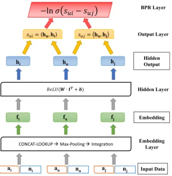
In this section, we discuss the proposed neural Bayesian personalized ranking model for attributed network embed-ding. The model uses a neural network architecture with embedding layer, hidden layer, output layer, and BPR layer from bottom to top, as illustrated in Fig. 1. Specifically, the embedding layer learns a unified vector representation of a node from the vector representation of its nodal attributes and neighbors; the hidden layer applies nonlinear dimen-sionality reduction over the embedding vectors of the nodes; the output layer and the BPR layer enable model inference through back-propagation.
4.1 Embedding Layer
The embedding layer has two embedding matrices 𝐏 and 𝐏′ ;
each row of 𝐏 is a d1-dimensional vector representation of
an attribute, and each row of 𝐏′ is a d2-dimensional vector
representation of a vertex (both d1 and d2 are user-defined
parameter). These matrices are updated iteratively during the learning process. For a given vertex u, embedding layer produces u’s latent representation vector 𝐟u by learning from
embedding vectors of u’s attributes and neighbors, i.e., cor-responding rows of 𝐏 and 𝐏′ , respectively; thus, the
neigh-bors and attributes of u are jointly involved in the construc-tion of u’s latent representation vector ( 𝐟u ), which enables
nodes with similar attributes and neighborhood in close proximity in the latent space.
We illustrate the vector construction process using a toy attributed graph in Fig. 2. Given the vertex b from the toy graph, the embedding layer first takes its attribute and adja-cency vectors (from 𝐏 and 𝐏′ ) as input and then generates its
corresponding attributional and nodal embedding matrices ( 𝐏(attr)
b and 𝐏 �(nbr)
b ) by using the CONCAT-LOOKUP(⋅)
func-tion. After that, attributional and neighborhood embedding vectors are obtained from 𝐏(attr)
b and 𝐏 �(nbr)
b by using the max
pooling operation, respectively. Finally, the learned attri-butional and neighborhood embedding vectors are concat-enated together to obtain the final embedding representation of the vertex b. Below we provide more details of the opera-tions in embedding layer.
4.1.1 Encoding Attributional Information
Given a node u∈V and the attribute matrix 𝐀 , 𝐚u ∈I R1×m
is 𝐀 ’s row corresponding to u’s binary attribute vector. We
apply a row-wise concatenation based embedding lookup layer to transform 𝐚u into a latent matrix, 𝐏(attr)
u , shown as
follows:
where 𝐏∈I Rm×d1 is the attribute embedding matrix in which
each row is a d1 (user-defined parameter) sized vector
repre-sentation of an attribute. Lookup is performed by CONCAT-LOOKUP(⋅) function which first performs a row projection
(1)
𝐏(attr)
u =CONCAT-LOOKUP(𝐏,𝐚u),
on 𝐏 by selecting the rows corresponding to the attribute
set A(u) and then stacks the selected vectors row-wise into
the matrix 𝐏(attr) u ∈I R|
A(u)|×d1 . Then we apply a max pooling
operation on the generated 𝐏(attr)
u matrix in order to transform
it into a single vector. Specifically, max pooling operation retains the most informative signal by extracting the largest value in each dimension (i.e., column) of the matrix 𝐏(attr)
u
to obtain 𝐯attr u .
where 𝐯attr u ∈I R
1×d1 is the latent vector representation of
node u based on its attributional signals and MP(⋅) denotes
the max pooling operation.
4.1.2 Encoding Network Topology
Given a node u, we describe its neighborhood by using a binary adjacency vector, denoted as 𝐧u∈I R1×n , in which u’s neighbors are set to 1, and the rest of entries are set as 0. Similar to the operations we use for encoding the attri-butional information, we apply a row-wise concatenation based lookup layer to transform 𝐧u into a latent matrix 𝐏�(nbr)
u
and then apply max pooling operation on the obtained latent matrix. Thus, (2) 𝐯attr u =MP(𝐏 (attr) u ), (3) 𝐏�(nbr) u =CONCAT-LOOKUP(𝐏 � ,𝐧u) BPR Layer Output Layer Hidden Layer Embedding Layer Input Data Embedding Hidden Output ni ai
CONCAT-LOOKUP Max-Pooling Integraon
fu fj fi ( ∙ + ) hu hj hi = , = , −ln − nu au aj nj
Fig. 1 Neural-Brane architecture. Given a node u, 𝐚
u is its binary
attribute vector and 𝐧
u is its adjacency vector. Our training uses node
triplets (u, i, j), such that (u,i) ∈E and (u,j) ∉E
1 0 1 1 0 0 1 0 0 0 1 Inputs ( ) ( ) ̵ ∙ [max−pooling] ⨁[concat] a e c d [x4] [x2, x4, x5] [x2, x6] [x2] [x1, x3, x7] b (1 × ) (3 × 2) (2 × 1) (1 × 1) (1 × 2) e a b c d 2 = 4 ′ x5 x6 x1 x2 x3 x4 x7 1 = 3 x2 x6 ( ) a c d ′ ( )
Fig. 2 Mechanism of the embedding layer for the vertex b of a toy attributed graph. The graph contains 5 vertices and 6 edges, where each vertex is associated with a collection of nodal attributes. For example, vertex b is connected to vertices {a,c,d} and associated
with attributes {x2,x6} , respectively. The cardinality of the attribute
where 𝐏�∈I Rn×d2 is the neighborhood embedding matrix
for lookup (similar to matrix 𝐏 ), and 𝐏�(nbr) u ∈I R|
N(u)|×d2 is
the obtained latent matrix generated from the CONCAT-LOOKUP(⋅) function. Moreover, 𝐯nbr
u ∈I R
1×d2 obtained
from the MP(⋅) operation is the latent vector representation
of node u based on its neighborhood topology.
4.1.3 Integration Component
Once we obtain the vector representation of node u from both its attributional information and topological structure as developed in Eqs. 1, 2, 3, and 4, we further integrate both latent vectors into a unified vector representation by vector concatenation, shown as follows:
where 𝐟u∈I R1×d ( d1+d2=d ) and “||” denotes the vector
concatenation operation.
4.2 Hidden Layer
Given the obtained embedding vector 𝐟𝐮∈I R1×d for node u
in the attributed network G, the hidden layer aims to trans-form its embedding vector into another representation 𝐡u , in
which signals from attributes and neighborhood of a vertex interact with each other. Formally, given 𝐟u , the hidden layer
produces 𝐡u∈I R1×h by the following formula:
Here we use rectified linear function ReLU(x), defined as max(0, x) , as the activation function for achieving better
convergence speed. Parameters 𝐖∈I Rh×d and 𝐛∈I Rh×1
are weights and bias for the hidden layer, respectively; h is a user-defined parameter denoting the number of neurons in the hidden layer. It is worth mentioning that in the hidden layer, all the nodes share the same set of parameters {𝐖,𝐛} ,
which enables information sharing across different vertices (see the box denoted as “hidden layer” in Fig. 1).
4.3 Output and BPR Layers
Given a node pair u and i, we use their corresponding repre-sentations 𝐡u and 𝐡i from hidden layer (Eq. 6) as input for the
output layer. The task of this layer is to measure the similar-ity score between a pair of vertices by taking the dot product of their representation vectors. Since this computation uses the vector representation of the vertices from the hidden layer, it encodes both attribute similarity and neighborhood similarity jointly. The similarity score between vertices u
and i, defined as sui , is calculated as ⟨𝐡u,𝐡i⟩.
(4) 𝐯nbr u =MP(𝐏 �(nbr) u ), (5) 𝐟u=𝐯attr u ||𝐯 nbr u ∶= [𝐯 attr u 𝐯 nbr u ], (6) 𝐡T u =ReLU(𝐖𝐟 T u +𝐛)
BPR layer implements the Bayesian personalized ranking objective. For the embedding task, the ranking objective is that the neighboring nodes in the graph should have more similar vector representations in the embedding space than non-neighboring nodes. For example, the similarity score between two neighboring vertices u and i should be larger than the similarity score between two non-neighboring nodes u and j. As shown in Fig. 1, given the vertex triplet (u, i, j), we model the probability of preserving ranking order
sui>s
uj using the sigmoid function 𝜎(x) = 1 1+e−x .
Mathematically,
As we observe from Eq. 7, the larger the difference between sui and suj , the more likely the ranking order sui>suj
is preserved. By assuming that all the triplet based rank-ing orders generated from the graph G to be independent, the probability of all the ranking orders being preserved is defined as follows:
where D represents training triplet sets generated from
G and i>uj is a shorthand notation denoting sui>suj ; the
notation is motivated from the concept that i is larger than j
considering the partial-order relation >
u.
The goal of our attributed network embedding is to maxi-mize the expression in Eq. 8. For the computational con-venience, we minimize the sum of negative likelihood loss function, which is shown as follows:
where 𝛩= {𝐏,𝐏�,𝐖,𝐛} are model parameters used in all
different layers and 𝜆
⋅||𝛩||2F is a regularization term to
pre-vent model overfitting.
4.4 Model Inference and Optimization
We employ the back-propagation algorithm by utilizing mini-batch gradient descent to optimize the parameters
𝛩= {𝐏,𝐏�,𝐖,𝐛} in our model. The first step of mini-batch
gradient descent is to sample a batch of triplets from G. Specifically, given an arbitrary node u, we sample one of its neighbors i, i.e., i∈N(u) , with the probability proportional
to the edge weight wij . On the other hand, we sample its
non-neighboring node j, i.e., j∉N(u) , with the
probabil-ity proportional to the node degree in the graph. Next, for each mini-batch training triplet, we compute the derivative (7) P�sui>suj�𝐡u,𝐡i,𝐡j�=𝜎�s ui−suj � = 1 1+e− � ⟨𝐡𝐮,𝐡 i⟩−⟨𝐡u,𝐡j⟩ � (8) ∏ (u,i,j)∈D P(i>uj) = ∏ (u,i,j)∈D 𝜎(sui−suj ) , (9) L(𝛩) =min 𝛩 − ∑ (u,i,j)∈D ln𝜎(s ui−suj ) +𝜆 ⋅||𝛩||2F
and update the corresponding parameters 𝛩 . For that, first
we find the gradient of the objective function in Eq. 9 with respect to model parameter
Now, for each model parameter we find 𝜕
𝜕𝛩(sui−suj)
using the chain rule. In particular, by back-propagating from Bayesian personalized ranking layer to hidden layer, we update the gradients w.r.t. weight matrix 𝐖 and bias
vec-tor 𝐛 accordingly. Then in the embedding layer, we update
the gradients of the corresponding embedding vectors (i.e., rows) in {𝐏,𝐏�} associated with all the neighboring nodes
and attributes involved in each mini-batch training triplet, respectively. Mathematically,
where 𝛼 is the learning rate. In addition, we initialize all
model parameters 𝛩 by using a Gaussian distribution with
0 mean and 0.01 standard deviation. The pseudo-code of the proposed Neural-Brane framework is summarized in Algorithm 1.
4.5 Model Complexity Analysis
For the time complexity analysis, given the sampled train-ing triplet set D , the total costs of calculating and
updat-ing gradients of L w.r.t. corresponding embedding vectors
involved in {𝐏,𝐏�} are O(d) . Similarly, the total costs of
(10) 𝜕L(𝛩) 𝜕𝛩 = − ∑ (u,i,j)∈D 𝜕ln𝜎(s ui−suj ) 𝜕𝛩 + 𝜆 𝜕||𝛩||2 F 𝜕𝛩 = − ∑ (u,i,j)∈D ( 1−𝜎(s ui−suj) ) ⋅ 𝜕 𝜕𝛩 ( sui−suj) +2𝜆||𝛩||F (11) 𝛩t+1 =𝛩t−𝛼×𝜕L(𝛩) 𝜕𝛩
computing and updating gradients of L w.r.t. parameters
{𝐖,𝐛} in the hidden layer are O(hd+h) . To generate
train-ing mini-batch, we use degree proportional sampltrain-ing and its time complexity is O(n) . Therefore, the total computational
complexity of the proposed methodology for Neural-Brane
is |D|∗(O(d) +O(hd+h) +O(n)) . As time complexity of
the Neural-Brane is linear to the embedding size, hidden layer dimension, and input graph size, it is extremely fast. For example, it takes around 15 minutes to learn embedding for our largest dataset Arnetminer (see Table 1). We can easily observe that the space complexity for the proposed
Neural-Brane is proportional to input graph size and embed-ding size, i.e., O(n⋅d).
5 Experiments and Results
In this section, we first introduce the datasets and baseline comparisons used in this work. Then we thoroughly evaluate our proposed Neural-Brane through two downstream data mining tasks (node classification and clustering) on four real-world networks, for which node attributes are available. Finally, we analyze the quantitative experimental results and investigate parameter sensitivity, convergence behavior, and the effect of pooling strategy of Neural-Brane.
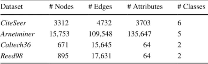
Table 1 Statistics of four real-world datasets
Dataset # Nodes # Edges # Attributes # Classes
CiteSeer 3312 4732 3703 6
Arnetminer 15,753 109,548 135,647 5
Caltech36 671 15,645 64 2
5.1 Experimental Setup 5.1.1 Datasets
We perform experiments on four real-world datasets, whose statistics are shown in Table 1. The largest among these net-works has around 15.75 K vertices and 109.5 K edges. Note that publicly available networks exist, which are larger than the networks that we use in this work, but those larger net-works are neither attributed nor they have class label for the vertices, so we cannot use those in our experiment. Nev-ertheless, our largest dataset Arnetminer has more nodes, edges, and attributes than datasets used by recent attribute embedding papers [23, 26]. More description of the datasets is given below.
CiteSeer1 is a citation network, in which nodes refer
to papers and links refer to citation relationship among papers. Selected keywords from the paper are used as nodal attributes. Additionally, the papers are classified into 6 cat-egories according to its research domain, namely artificial intelligence (AI), database (DB), information retrieval (IR), machine learning (ML), human computer interaction (HCI), and multi-agent analysis.
Arnetminer2 is a paper relation network consisting of
scientific publications from 5 distinct research areas. Spe-cifically, we select a list of representative conferences and journals from each of them. (1) Data Mining (KDD, SDM, ICDM, WSDM, PKDD); (2) Medical Informatics (JAMIA, J. of Biomedical Info., AI in Medicine, IEEE Tran. on Medi-cal Imaging, IEEE Tran. on Information and Technology in Biomedicine); (3) Theory (STOC, FOCS, SODA); (4)
Computer Vision and Visualization (CVPR, ICCV, VAST, TVCG, IEEE Visualization and Information Visualization); (5) Database (SIGMOD, VLDB, ICDE). Authors and key-words similarity between two papers are used for building edges. Keywords from paper title and abstract are used as attributes.
Caltech36 and Reed98 [19] are two university Face-book networks. Specifically, each node represents a user from the corresponding university and edge represents user friendship. The attributes of each node are represented by a 64-dimensional one-hot vector based on gender, major, second major/minor, dorm/house, and year. We use student/ faculty status of a node as the class label.
5.1.2 Baseline Comparison
To validate the benefit of our proposed Neural-Brane, we compare it against 10 different methods. Among all the
competing methods, DeepWalk, LINE, and Node2Vec are topology-oriented network embedding approaches. NNMF, DeepWalk + NNMF, GraphSAGE, PTE-KL, TADW, AANE, and G2G are state of the arts for combining both network structure and nodal attributes for network repre-sentation learning. Note that PTE-KL is a semi-supervised embedding approach, and we hold the label information out for a fair comparison.
1. DeepWalk [15]: It utilizes Skip-Gram based language model to analyze the truncated uniform random walks on the graph.
2. LINE [18]: It embeds the network into a latent space by leveraging both first-order and second-order proximi-ties of each node.
3. Node2Vec [9]: Similar to DeepWalk, Node2Vec designs a biased random walk procedure for network embedding.
4. Non-Negative Matrix Factorization (NNMF): The model captures both node attributes and network struc-ture to learn topic distributions of each node.
5. DW+NNMF: It simply concatenates the vector repre-sentations learned by DeepWalk and NNMF.
6. GraphSAGE [10]: GraphSAGE presents an inductive representation learning framework that leverages node feature information (e.g., text attributes) to efficiently generate node embeddings in the network.
7. PTE-KL [17]: Predictive Text Embedding framework aims to capture the relations of paper–paper and paper– attribute under matrix factorization framework. The objective is based on KL divergence between empirical similarity distribution and embedding similarity distri-bution.
8. TADW [23]: Text-Associated DeepWalk combines the text features of each node with its topology information and uses the MF version of DeepWalk.
9. AANE [12]: Accelerated Attributed Network Embed-ding learns low-dimensional representation of nodes from network linkage and content information through a joint matrix factorization.
10. G2G [2]: Graph2Gauss learns node representation such that each node vector is a Gaussian distribution.
5.1.3 Parameter Setting and Implementation Details
There are a few user-defined hyper-parameters in our pro-posed embedding model. We fix the embedding dimension
d=150 (same for all baseline methods) with d1=d2=75 .
For the number of neurons in hidden layer h, we set it to be 150. For the regularization coefficient 𝜆 in the embedding
model (see Eq. 9), we set it as 0.00005. In addition to that,
1 https ://linqs .soe.ucsc.edu/data. 2 https ://amine r.org/topic _paper _autho r.
we fix the learning rate 𝛼=0.5 (see Eq. 11) and batch size
to be 100 during the model learning and optimization. For baseline methods such as GraphSAGE, PTE-KL, AANE, G2G and others, we select learning rate 𝛼 from the set {0.01, 0.05, 0.1, 0.5}3 using grid search. Similarly for
PTE-KL, TADW and other baseline methods regularization coef-ficient 𝜆 is selected from the set {0.01, 0.001, 0.0001} . For
random walk based baselines (DeepWalk and Node2Vec), we select the best walk length from the set {20, 40, 60, 80} .
For the rest of hyper-parameters, we use default parameter values as suggested by their original papers.
5.2 Quantitative Results 5.2.1 Node Classification
For fair comparison between network embedding methods, we purposely choose a linear classifier to control the impact of complicated learning approaches on the classification performance. Specifically, we treat the node representations
learned by different approaches as features and train a logis-tic regression classifier for multi-class/binary classification. In each dataset, p% ∈ {30%, 50%, 70%} of nodes are
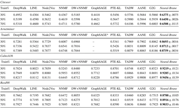
ran-domly selected as training set and the rest as test set. We use the widely used metric Macro-F1 [24] for classifica-tion assessment. Each method is executed 10 times, and the average value is reported. For Neural-Brane, we also report standard deviation. For better visual comparison, we high-light the best Macro-F1 score of each training ratio (p) with bold font.
Table 2 shows results for node classification, where each column is an embedding method and rows represent different train splits (p). As we observe from Table 2, per-formance of the last four (PTE-KL, TADW, AANE, G2G) baseline methods is highly competitive among each other. But, our proposed Neural-Brane consistently outperforms all these and other baseline methods under all training ratios. Moreover, the overall performance improvement that our
Neural-Brane delivers over the second best method is sig-nificant. For example, in Citeseer dataset, when training ratio
p ranges from 30% to 70% , Neural-Brane outperforms the
G2G by 8.8% , 8.6% , 8.4% in terms of Macro-F1, respectively.
Furthermore, the improvement over G2G is statistically sig-nificant (paired t-test with p-value ≪ 0.01). The relatively Table 2 Quantitative results of Macro-F1 between our proposed Neural-Brane and other baselines for the node classification task using logistic regression on various datasets (embedding dimension = 150)
*GraphSAGE for Arnetminer is not able to complete after 2 days
Citeseer
Train% DeepWalk LINE Node2Vec NNMF DW+NNMF GraphSAGE PTE-KL TADW AANE G2G Neural-Brane 30% 0.4952 0.4304 0.5462 0.4367 0.5185 0.4418 0.5456 0.5756 0.5684 0.5860 𝟎.𝟔𝟑𝟕𝟓±.0075 50% 0.5199 0.4590 0.5632 0.4619 0.5598 0.4621 0.5647 0.5900 0.5844 0.5939 𝟎.𝟔𝟒𝟓𝟎±.0026 70% 0.5318 0.4600 0.5743 0.4711 0.5780 0.4662 0.5732 0.6106 0.5996 0.6003 𝟎.𝟔𝟓𝟎𝟖±.0115 Arnetminer
Train% DeepWalk LINE Node2Vec NNMF DW+NNMF GraphSAGE* PTE-KL TADW AANE G2G Neural-Brane 30% 0.7281 0.5364 0.7729 0.6087 0.6968 – 0.5341 0.7969 0.7902 0.8062 𝟎.𝟖𝟔𝟗𝟑±.0016 50% 0.7336 0.5422 0.7837 0.6541 0.7016 – 0.5426 0.8031 0.8009 0.8145 𝟎.𝟖𝟕𝟏𝟑±.0017
70% 0.7389 0.5485 0.7877 0.6748 0.7044 – 0.5519 0.8079 0.8065 0.8186 𝟎.𝟖𝟕𝟓𝟗±.0034 Caltech36
Train% DeepWalk LINE Node2Vec NNMF DW+NNMF GraphSAGE PTE-KL TADW AANE G2G Neural-Brane 30% 0.7824 0.8023 0.7859 0.5243 0.8480 0.7233 0.8701 0.8748 0.8527 0.8523 𝟎.𝟗𝟐𝟏𝟗±.0121 50% 0.7949 0.8079 0.8080 0.5953 0.8552 0.7712 0.8697 0.8866 0.8843 0.8691 𝟎.𝟗𝟐𝟖𝟓±.0134 70% 0.8217 0.8112 0.8131 0.6445 0.8712 0.8220 0.8786 0.8929 0.9008 0.8977 𝟎.𝟗𝟒𝟓𝟔±.0139 Reed98
Train% DeepWalk LINE Node2Vec NNMF DW+NNMF GraphSAGE PTE-KL TADW AANE G2G Neural-Brane 30% 0.7662 0.7195 0.7682 0.6472 0.8055 0.6325 0.8333 0.8460 0.8285 0.7515 𝟎.𝟖𝟕𝟖𝟖±.0105 50% 0.7774 0.7195 0.7805 0.7123 0.8275 0.7012 0.8413 0.8519 0.8433 0.7772 𝟎.𝟖𝟗𝟏𝟔±.0176
70% 0.7927 0.7446 0.7925 0.7695 0.8321 0.7682 0.8590 0.8636 0.8660 0.7925 𝟎.𝟗𝟎𝟑𝟑±.0146
3 For GraphSAGE, we also check smaller values of 𝛼 , i.e.,
good performance of our proposed Neural-Brane across various training ratios is due to the fact that our proposed neural Bayesian personalized ranking framework is able to generate high-quality latent features by capturing crucial ordering information between nodes and incorporating nodal attributes and network topology into network embedding. Furthermore, BPR is shown to be better suited than other loss functions, such as point-wise square loss in TADW and KL divergence based objective in LINE and PTE-KL, for placing similar nodes in the embedding space for the down-stream node classification task.
Among the competing methods, topology-oriented net-work embedding approaches such as LINE and DeepWalk perform fairly poor on all datasets. This is mainly because the network structure is rather sparse and only contains lim-ited information. On the other hand, TADW is much better than DeepWalk due to the fact that textual contents contain richer signals compared to the network structure. When concatenating the embedding vectors from DeepWalk and NNMF, the classification performance is relatively improved compared to a single DeepWalk. However, the naive combi-nation between DeepWalk and NNMF is far from optimal, compared to our proposed Neural-Brane. Note that Graph-SAGE for Arnetminer dataset is not able to complete after 2
days on contemporary server having 64 cores with 2.3 GHz and 132 GB memory.
5.2.2 Visualization and Node Clustering
The primary goal of graph embedding approaches is to put similar nodes closer in their corresponding latent space; hence, a desirable embedding method should generate clus-ters of similar nodes in the embedding space. Visualization for a large number of classes in two-dimensional space is impractical. Instead, in Fig. 3, we plot 2D representation of learned vector representations for Caltech36 and Reed98
datasets. Note that both of these datasets contain only 2 classes and hence provide interpretable visualization. Specif-ically, we plot embedding representations of Neural-Brane
along with two best competing methods, namely TADW and AANE. These figures clearly demonstrate that Neural-Brane
provides better discrimination of classes through clustering in the latent space compared to both TADW and AANE.
For the other two larger datasets (CiteSeer and Arnet-miner), we use k-means clustering approach to the learned vector representations of nodes and utilize both Purity and Normalized Mutual Information (NMI) [24] to assess the quality of clustering results. Furthermore, we match the ground truth number of clusters as input for running
(a)Representation of TADW
forCaltech36 (b)forRepresentation of AANECaltech36 (c)BraneRepresentation offorCaltech36
Neural-(d)Representation of TADW
forReed98 (e)forRepresentation of AANEReed98 (f)BraneRepresentation offorReed98
k-means, execute the clustering process 10 times to allevi-ate the sensitivity of centroid initialization, and report the average results.
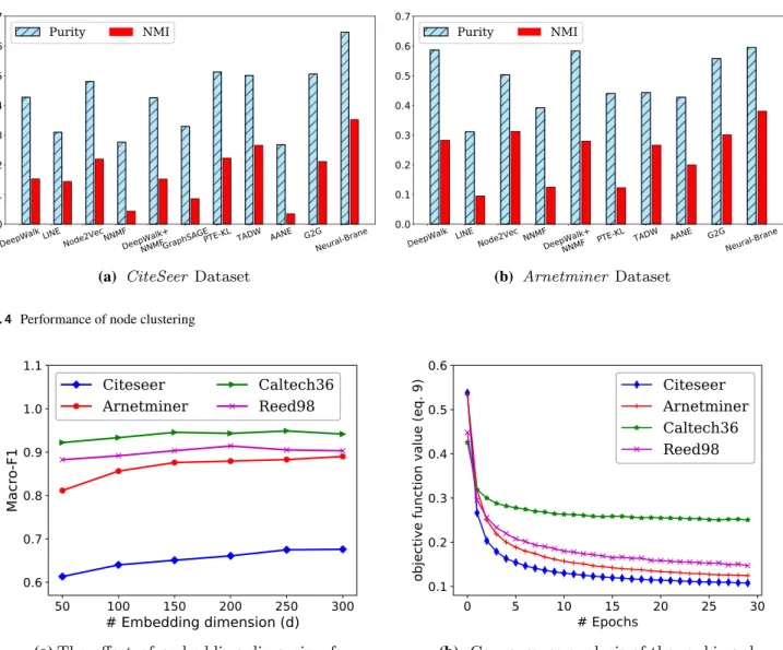
The clustering results for both CiteSeer and Arnetminer
datasets are depicted in Fig. 4. As we can see, our proposed
Neural-Brane consistently achieves the best clustering results in contrast to all competing baselines. For example, in Citeseer dataset, our proposed Neural-Brane achieves 0.3524 NMI. However, the best competing method PTE-KL only obtains 0.2653 NMI, indicating more than 32.8%
gains. Similarly, for Arnetminer dataset, Neural-Brane
obtains 34.5% improvements over the best competing
approach DeepWalk in terms of NMI. The possible expla-nation for higher performance of Neural-Brane could be due to the fact that our proposed Bayesian ranking formulation directly optimizes the pair-wise distance between similar and
dissimilar nodes, thus making their corresponding vectors cluster-aware in the embedded space.
5.3 Analysis of Parameter Sensitivity and Algorithm Convergence
We conduct experiments to demonstrate how the embed-ding dimension affects the node classification task using our proposed Neural-Brane. Specifically, we vary the number of embedding dimension parameter d as
{50, 100, 150, 200, 250, 300} and set the training ratio p=70% . We report the Macro-F1 results on all four
data-sets, which is shown in Fig. 5a. As we observe, as the embedding dimension d increases, the classification perfor-mance in terms of Macro-F1 first increases and then tends to stabilize. The possible explanation could be that when
(a) CiteSeer Dataset (b) Arnetminer Dataset
Fig. 4 Performance of node clustering
(a) The effect of embedding dimension for
node classification (b)jective function shown in Equation 9 Convergence analysis of the ranking
the embedding dimension is too small, the embedding rep-resentation capability is not sufficient. However, when the embedding dimension becomes sufficiently large, it captures all necessary information from the data, leading to the stable classification performance. Furthermore, we investigate the convergence trend of Neural-Brane. As shown in Fig. 6b,
Neural-Brane converges approximately within 10 epochs and achieves promising convergence results in terms of the objective function value on all four datasets.
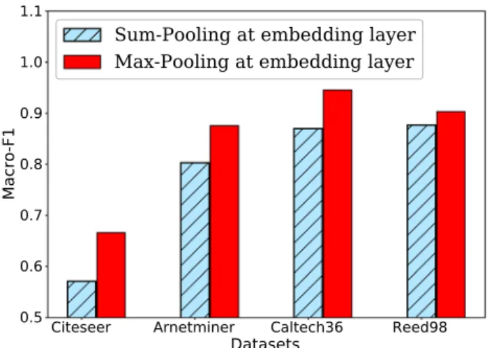
5.4 Effect of Pooling Strategy and Number of Training Triples
We investigate the effect of the pooling strategy in the embedding layer for the task of node classification. For the comparison, we consider to take the sum rather than max pooling and hold the rest of neural architecture and
hyper-parameter settings constant. We report the Macro-F1 results on all four datasets with training ratio p=70% ,
which is shown in Fig. 7a. As we observe, max pooling con-sistently outperforms the alternative sum pooling strategy for the task of node classification across all datasets. The possible explanation is due to the fact that the max pool-ing operation returns the strongest signal for each embed-ding dimension, which alleviates noisy signals. On the other hand, the sum pooling operation considers accumulated sig-nals from each input embedding dimension, which leads to inaccurate information aggregation.
Finally, to verify the efficiency of the Neural-Brane, we study how embedding generation time and node classifica-tion performance vary with count of training triples. For that, we use Arnetminer dataset and plot macro-F1 results and embedding generation time over different counts of training triples in Fig. 7b. We can see that for half a million
(a)The pooling strategy comparison for the
task of node classification (b)performance and time (ArnetminerEffect of # triples used for training ondataset)
Fig. 6 Study effects of pooling strategy and # training triples
(a) Results for scalability study
(b) Results of performance using different loss functions
(c) Combined and indepen-dent learning of attribute and neighborhood embedding.
triples the Neural-Brane doesn’t render the optimal result as the method is not converged. However, it converges with 1.5 million triples and consistently provides very good perfor-mance (high Macro-F1) for higher triple counts. Notice that, for this biggest dataset (Arnetminer), Neural-Brane takes around 6 minutes ( <400 seconds) to sample the 1.5 million
triples and train with those triples. This observation also proves that Neural-Brane is highly scalable because of its linear time complexity (Sect. 4.5).
5.5 Scalability Study
To check the scalability of the proposed Neural-Brane, we conducted experiment to check run times of various large synthetic networks. To generate these synthetic networks, we use popular Barabási–Albert preferential attachment model [1]. We generate low density random binary vector of size 500 as a synthetic attributes for each node. For this experiment, we vary size of the networks such that they have nodes in range of 25,000 to 100,000 with 25,000 increment. The running time of these networks is depicted in Fig. 7a, which shows a linear increase in run time with the increase in size of the network. The empirical linear increase in run time with respect to the size of the network is consistent with our model complexity analysis in Sect. 4.5.
5.6 Effectiveness of BPR Loss and Contribution of Other Neural‑Brane layers
As we discussed before, the ranking BPR loss as an objec-tive function highly contributes toward the remarkable performance of the proposed Neural-Brane. To support this claim, we conduct comparison experiment where we replace the objective function of the Neural-Brane with tra-ditional Hinge loss and Cross-entropy (Log) loss. For fair comparison, we run the modified models with the same set of parameters discussed in Sect. 5.1.2. The performance of the modified methods and proposed Neural-Brane is shown in Fig. 7b, where we can see that Neural-Brane with BPR loss always outperforms both Log loss- and Hinge loss based methods.
Though BPR loss helps in performance improvement in the Neural-Brane, we need to check the importance of embedding and hidden layers which are responsible for information fusion of topology and attributes. For this experiment, we feed attribute vector ( vattr
b for node b)
directly to the output layer to learn attribute embedding ( 𝐏 ). Similarly, we feed neighborhood vector ( vnbr
b for node b) to output layer to learn neighborhood based embedding ( 𝐏′ ). We concatenate these vectors for each node as a final
node representation vectors; we call this method as node & attribute separate embedding. We compare the classifica-tion performance of this embedding method with proposed
Neural-Brane, and results are shown in Fig. 7c. This com-parison result shows that the embedding and hidden layers of the proposed method contribute toward improvement in the performance. Hence, from these results, we can conclude that both BPR loss as an objective function and advanced approach of information fusion using embedding and hidden layers jointly produce superior performance for the proposed
Neural-Brane.
6 Conclusion
We present a novel neural Bayesian personalized ranking formulation for attributed network embedding, which we call Neural-Brane. Specifically, Neural-Brane combines a designed neural network model and a novel Bayesian rank-ing objective to learn informative vector representations that jointly incorporate network topology and nodal attributions. Experimental results on the node classification and clus-tering tasks over four real-world datasets demonstrate the effectiveness of the proposed Neural-Brane over 10 baseline methods.
Funding Funding was provided by Indiana University (Grant No. IU-Bridge research grant).
Open Access This article is distributed under the terms of the
Crea-tive Commons Attribution 4.0 International License (http://creat iveco mmons .org/licen ses/by/4.0/), which permits unrestricted use, distribu-tion, and reproduction in any medium, provided you give appropriate credit to the original author(s) and the source, provide a link to the Creative Commons license, and indicate if changes were made.
References
1. Barabási AL, Albert R (1999) Emergence of scaling in random networks. Science 286(5439):509–512
2. Bojchevski A, Günnemann S (2018) Deep gaussian embedding of graphs: unsupervised inductive learning via ranking. In: Inter-national conference on learning representations (ICLR) 3. Cao S, Lu W, Xu Q (2015) Grarep: Learning graph
representa-tions with global structural information. In: ACM International on conference on information and knowledge management, pp 891–900
4. Cao S, Lu W, Xu Q (2016) Deep neural networks for learning graph representations. In: AAAI, pp 1145–1152
5. Chang S, Han W, Tang J, Qi GJ, Aggarwal CC, Huang TS (2015) Heterogeneous network embedding via deep architectures. In: International conference on knowledge discovery and data min-ing, pp 119–128
6. Dave V, Zhang B, Hasan MA, Jadda KA, Korayem M (2018) A combined representation learning approach for better job and skill recommendation. In: ACM conference on information and knowledge management
7. García-Durán A, Niepert M (2017) Learning graph representa-tions with embedding propagation. In: NIPS, pp 5125–5136 8. Goyal P, Ferrara E (2017) Graph embedding techniques,
9. Grover A, Leskovec J (2016) Node2vec: scalable feature learn-ing for networks. In: ACM SIGKDD international conference on knowledge discovery and data mining, KDD ’16, pp 855–864 10. Hamilton W, Ying Z, Leskovec J (2017) Inductive
representa-tion learning on large graphs. Adv Neural Inf Process Syst 30:1024–1034
11. Hamilton WL, Ying R, Leskovec J (2017) Representation learn-ing on graphs: methods and applications. IEEE Data Eng Bull 40(3):52–74
12. Huang X, Li J, Hu X (2017) Accelerated attributed network embedding. In: SIAM international conference on data mining, pp 633–641
13. Huang X, Li J, Hu X (2017) Label informed attributed network embedding. In: ACM international conference on web search and data mining, pp 731–739
14. Pan S, Wu J, Zhu X, Zhang C, Wang Y (2016) Tri-party deep net-work representation. In: International joint conference on artificial intelligence, pp 1895–1901
15. Perozzi B, Al-Rfou R, Skiena S (2014) Deepwalk: online learning of social representations. In: ACM SIGKDD international con-ference on knowledge discovery and data mining, KDD ’14, pp 701–710
16. Rendle S, Freudenthaler C, Gantner Z, Schmidt-Thieme L (2009) Bpr: Bayesian personalized ranking from implicit feedback. In: Conference on uncertainty in artificial intelligence, UAI ’09, pp 452–461
17. Tang J, Qu M, Mei Q (2015) Pte: Predictive text embedding through large-scale heterogeneous text networks. In: SIGKDD, pp 1165–1174
18. Tang J, Qu M, Wang M, Zhang M, Yan J, Mei Q (2015) Line: large-scale information network embedding. In: International con-ference on world wide web, WWW ’15, pp 1067–1077 19. Traud AL, Mucha PJ, Porter MA (2012) Social structure of
face-book networks. Physica A: Stat Mech Appl 391(16):4165–4180 20. Tu C, Zhang W, Liu Z, Sun M (2016) Max-margin deepwalk:
discriminative learning of network representation. In: IJCAI, pp 3889–3895
21. Wang D, Cui P, Zhu W (2016) Structural deep network embed-ding. In: SIGKDD international conference on knowledge discov-ery and data mining, KDD ’16, pp 1225–1234
22. Wang X, Cui P, Wang J, Pei J, Zhu W, Yang S (2017) Community preserving network embedding. In: AAAI conference on artificial intelligence
23. Yang C, Liu Z, Zhao D, Sun M, Chang EY (2015) Network rep-resentation learning with rich text information. In: International conference on artificial intelligence, IJCAI’15, pp 2111–2117 24. Zaki MJ, Meira W Jr (2014) Data mining and analysis:
funda-mental concepts and algorithms. Cambridge University Press, Cambridge
25. Zhang B, Al Hasan M (2017) Name disambiguation in anonymized graphs using network embedding. In: ACM on conference on information and knowledge management, pp 1239–1248
26. Zhang D, Yin J, Zhu X, Zhang C (2017) User profile preserving social network embedding. In: International joint conference on artificial intelligence, IJCAI-17, pp 3378–3384