1
Chance-constrained Cost Efficiency in Data Envelopment
Analysis model with random inputs and outputs
Rashed Khanjani Shiraz1, Adel Hatami-Marbini2, Ali Emrouznejad3, Hirofumi Fukuyama4
1 School of Mathematical Science, University of Tabriz, Tabriz, Iran, [email protected] 2 Department of Strategic Management and Marketing, Leicester Business School, De Montfort
University, Hugh Aston Building, The Gateway, Leicester LE1 9BH, UK, [email protected]
3 Operations and Information Management Group, Aston Business School, Aston University, Birmingham, UK, [email protected]
4 Faculty of Commerce, Fukuoka University, 8-19-1 Nanakuma, Jonan-Ku, Fukuoka City, Fukuoka 814-0180, Japan, [email protected]
Abstract
Data envelopment analysis (DEA) is a well-known non-parametric technique primarily used to estimate radial efficiency under a set of mild assumptions regarding the production possibility set and the production function. The technical efficiency measure can be complemented with a consistent radial metrics for cost, revenue and profit efficiency in DEA, but only for the setting with known input and output prices. In many real applications of performance measurement, such as the evaluation of utilities, banks and supply chain operations, the input and/or output data are often stochastic and linked to exogenous random variables. It is known from standard results in stochastic programming that rankings of stochastic functions are biased if expected values are used for key parameters. In this paper, we propose economic efficiency measures for stochastic data with known input and output prices. We transform the stochastic economic efficiency models into a deterministic equivalent non-linear form that can be simplified to a deterministic programming with quadratic constraints. An application for a cost minimizing planning problem of a state government in the US is presented to illustrate the applicability of the proposed framework.
Keywords: Data envelopment analysis; Weight restrictions; random input-output; Cost efficiency; Quadratic programming.
2
1. Introduction
Data envelopment analysis (DEA) is recognized as a powerful analytical tool that is widely used in measuring the relative efficiency of a group of decision making units (DMUs) with multiple inputs and multiple outputs. The first DEA model has been presented by Charnes et al. (1978) in the case of constant returns to scale (CRS) and later extended by Banker et al. (1984) in the case of variable returns to scale (VRS) for evaluating the technical efficiency of a set of comparable DMUs. A substantial number of DEA studies have been rapidly developed since 1978 and the evolution of the DEA scientific area can be found in Cook and Seiford (2009), Emrouznejad and De Witte (2010) and Liu et al. (2013).
In the conventional input-oriented DEA models1, the efficiency of the DMU to be evaluated is measured by making a comparison of its observed input vector with a projected point on an input-isoquant. That is, DEA emphasizes technical efficiency measurement by utilizing the radial measures, which are gauged relative to the input-isoquant by seeking the maximal equi-proportional reduction in all the inputs of the DMU that would be feasible for a given output vector. However, the radial input projection corresponding to the input-isoquant may not be located on the efficient (Pareto-Koopmans) input-frontier. Hence, after obtaining the radial projection, solving an additional optimization problem is needed. More precisely, in the radial-based DEA, it is common to use a two-phase procedure where the radial efficiency is estimated in the first phase and the input slack maximization problem is solved in the second phase. An alternative procedure is maximization of input slack by directly solving slack-based measures or input-oriented additive model. In either way, a projection point slack-based on only input slacks (input surpluses) may not be a cost-minimizing vector, which is very important from the economic theoretic and managerial viewpoints. Cost minimization refers to the firm’s decisions on the choice of input quantities given its output level and input prices.
Consider DMUs that minimize costs but do not maximize profits. Such DMUs include, not only non-profit organizations and cooperative firms, but also firms which for example struggle under economic depression and hence the output expansion is not possible. Under cost minimization, management chooses efficient input combinations but beyond that no particular criterion is implemented for choosing a specific output combination (Luenberger 1995). As is well-known, in competitive input and output markets profit maximization implies cost minimization but not vice versa.
According to microeconomic theory, marginal, average and total cost functions are major
3
tools for production analysis, implying that cost minimization is one of the basic norms in economic analysis. However, in real world situations, there exist inefficient firms due to excess use of their input-mix, in which case it is necessary to provide them with optimal input bundles.
For managers of economic entities too, taking cost performance into account is of great necessity because cost minimizing behaviour is at the core of managerial objectives. However, achieving such an objective may not be easy when they face uncertainty in data for which case the standard cost efficiency (CE) analysis cannot provide a practical solution. This necessitates implementing the stochastic nature in CE analysis.
A variety of production-based DEA models of stochastic programming have been developed for performance evaluation of DMUs in the various fields with different types of data such as deterministic, imprecise, interval and fuzzy data. Charnes and Cooper’s (1959) stochastic programming2 is one of the most commonly used methods. In order to enhance the practicality, Charnes and Cooper (1963) further presented a chance-constrained programming (CCP) model, in which a stochastic linear programming problem was transformed into a deterministic non-linear programming problem, and it was first utilized by Land et al. (1993) to deal with data stochasticity in production-based DEA.
Cooper et al. (2000a, b, 2004) further extended the CCP model into a congestion framework in DEA. While we recognise the usefulness of CCP, there does not exist any cost-based chance-constrained DEA model, which has the good theoretical foundation as well as good practicality. Therefore, we propose a cost-based DEA model that directly deals with stochastic input and output data for the purpose of increasing the realism of the CE analysis. To the best of our knowledge, the present study is the first one to develop a CE-DEA model using the stochastic input and output data along the line of chance-constrained programming introduced by Charnes and Cooper (1963) and Cooper et al. (1996). Our extension adapts Cooper et al.’s (2002a, b, 2004) production-based approach.
To show the applicability of our model we provide an illustrative example using the data provided by Ray et al. (2008). The dataset consists of US state-level data collected from the Economic Census. Although the original data values are nonstochastic and single-valued, we show how to use them for a planning purpose by introducing stochasticity in the data.
2Stochastic programming has been nowadays extended into numerous disciplines including
4
The remainder of this paper is organized as follows: In Section 2, we present a brief literature survey. In Section 3 we provide a review of the principle DEA models. Section 4 presents an extension of CE with stochastic input and output data.In Section 5, we develop a slack-based version of CE in the presence of stochastic data. Section 6 is dedicatedto illustrate the application of the proposed approach using a case study for a cost minimizing planning problem of a state government in the US. Section 7finallyconcludes our work and points out some directions of further work.
2. Selective literature
Some observations can be located on the efficient frontier in the deterministic DEA, while some stochastic inputs and outputs are by definition allowed to be around the efficient frontier can be allowed with the aim of conceptualizing the stochastic nature of the data into the model to adapt the measurement and specification errors. Stochastic input and output variations in DEA have been studied within various input-output DEA contexts by many scholars (see e.g., Olesen and Petersen, 2015, Olesen and Petersen, 1995; Huang and Li, 1996; Cooper et al., 1996, 1998, 2002, 2004; Land et al., 1993; Morita and Seiford, 1999; Sueyoshi, 2000; Talluri et al., 2006; Olesen, 2006; Bruni et al., 2009; Wu and Lee, 2010; Tsionas and Papadakis, 2010; Udhayakumar et al., 2011).
Land et al. (1993) were the first to extend the chance-constrained programming (CCP) DEA proposed by Charnes and Cooper (1959), in order to compute efficiency in the presence of uncertainty in which inputs are assumed to be deterministic and outputs are jointly normally distributed. The CCP DEA is a non-parametric approach to evaluate the efficiency while stochastic frontier analysis (SFA) is an alternative parametric approach. The parametric approach puts emphasis on the production or cost function along with studying the characteristics of the functions under the presumption that all DMUs operate under rational behavior. In the literature, relatively few papers on efficiency analysis have analytically compared parametric and non-parametric approaches (e.g., Bjurek et al. 1990; Cooper and Tone 1997). Bjurek et al. (1990) argued that there is no significant difference between deterministic DEA and a loglinear parametric model. Cooper and Tone (1997) discussed DEA and stochastic cost functions, identifying some particular problems of bias in SFA approaches.
To measure the efficiency, several researchers have further extended the concept of the stochastic production function. Coelli (1996) presented a method to estimate the maximum likelihood estimator of SFA developed by Battese and Coelli (1992). In SFA, the inefficiency
5
effect can be used as how far the DMU operates below the frontier production function. Coelli (1996) indicated that the inefficiency effects can be referred to as the technical inefficiency. Olesen and Petersen (1995) developed a chance constrained DEA model by imposing chance constraints on the multiplier model. Cooper et al. (1996) presented a joint chance constraints programming model in the multiplier DEA model. They used “satisficing concepts” presented by Simon (1957) to develop the potential applications of DEA models to situations where 100% efficiency can be replaced by aspired levels of performance. Huang and Li (1996) proposed a dominance structure to remove the anomalous (Pareto) efficient DMUs from the DEA envelopment side where input and output data are characterized by random variations. Cooper et al. (1998) introduced the “alpha-stochastic efficiency” and “alpha-stochastic efficiency dominance” of a DMU in stochastic DEA using the joint chance constraints where random disturbances are applied in the inputs and outputs on the assumption that the statistical distributions of data are known. Morita and Seiford (1999) studied robustness of the efficiency results when input and output data are subject to the stochastic measurement error. Sueyoshi (2000) put forward a stochastic DEA model to restructure strategy of a Japanese petroleum company, which is reformulated in the manner that ex ante information can be incorporated into the stochastic model. Cooper et al. (2002a) proposed a generalization of Cooper et al. (2002b)’s CCP model for identifying the technical efficiencies and inefficiencies. Cooper et al. (2004) extended congestion in DEA models based on CCP models. Talluri et al. (2006) applied chance constrained DEA model for vendor evaluation. Olesen (2006) presented a comparison of two different models (Land et al., 1993; Olesen and Petersen, 1995), both designed to extend DEA to the case of stochastic inputs and outputs. Lahdelma and Salminen (2006) proposed the SMAA-D method by combining DEA and SMAA-2 (stochastic multicriteria acceptability analysis) presented in (Lahdelma et al. 1998; Lahdelma and Salminen, 2001) which can be dealt with uncertain or imprecise data to provide stochastic efficiency measures. Bruni et al. (2009) proposed a stochastic DEA model based on the theory of joint probabilistic constraints to extend the concept of ‘‘Stochastic efficiency’’ to a measure called “alpha-stochastic efficiency”. Udhayakumar et al. (2011) exploited the genetic algorithm method to solve the chance constrained DEA model, which involves the concept of satisficing.
Tavana et al. (2012) developed three imprecise DEA models in the presence of probability-possibility, probability-necessity and probability-credibility constraints where fuzziness and randomness simultaneously are allowed to exist in an efficiency evaluation problem. Tavanaet
6
al. (2013) introduced random fuzzy variables in DEA with the coexistence of randomness and vagueness. In this respect, they proposed three DEA models for measuring the radial efficiency of DMUs when the input and output data are random fuzzy variables with Poisson, uniform and normal distributions. Tavana et al. (2014) proposed a chance-constrained DEA model with birandom input and output data as well as formulating a super-efficiency model with birandom constraints that was solved by means of an equivalent non-linear deterministic model.
Although many contributions in CE have been reported in the DEA literature (see, e.g., Färe et al., 1985; Schaffnitet al., 1997; Jahanshahloo et al., 2008; Thompson et al., 1996; Camanho and Dyson, 2008), only a few researchers have considered uncertainty in the CE context (see e.g., Kuosmanen and Post 2001, 2002, 2003; Camanho and Dyson 2005; Mostafaee and Saljooghi, 2010). Kuosmanen and Post (2001) developed a DEA-based method to determine the upper and lower bounds for overall economic efficiency and allocative efficiency with incomplete price data in the form of a convex polyhedral cone. Kuosmanen and Post (2003) corrected a technical error concerning the lower bound of Kuosmanen and Post (2001). Kuosmanen and Post (2002) discussed necessary and sufficient first-order stochastic dominance (FSD) efficiency conditions for economic efficiency with regarding the preferences of the decision-maker and the statistical distribution of the prices. Camanho and Dyson (2005) developed weight restrictions methods for estimating cost efficiency bounds in complex scenarios of input price uncertainty under the assumption that input prices are in the form of ranges. However, Camanho and Dyson’s (2005) model is not only computationally expensive but also may produce an infeasible solution (Mostafaee and Saljooghi, 2010. Amirteimoori et al (2006) proposed two DEA-based models to obtain the upper and lower bound of cost efficiency of each DMU with respect to the optimistic and pessimistic viewpoints, respectively. They then introduced a two-step procedure to improve the cost efficiency of DMUs.
Mostafaee and Saljooghi (2010) proposed a pair of two-level mathematical programming models to obtain the upper and lower bounds of the cost efficiency where the uncertain input prices are in the form of ranges. Bagherzadeh Valami (2009) provided an approach for generalizing the CE of DMUs when input prices are characterized by triangular fuzzy numbers. Fang and Li (2012) presented some counterexamples to show that the theorem of Mostafaee and Saljooghi (2010) on determination of the upper bound of CE is not correct in general and they then provided an alternative proof to clarify the reason. Fang and Li (2013)
7
studies the theoretical properties on the relationships and characteristics of the efficiency solutions between cone-ratio DEA models and CE models in situations of price uncertainty, where the upper and lower bounds of the input prices can be estimated for each DMU. They additionally developed a method and a lexicographic order algorithm based on the duality study to estimate the lower bounds of the CE measure.
The above literature shows the lack of much attention to the CE analysis under uncertainty due to the degrees of complexity while real-world problems often include uncertain data, particularly the cases with stochastic input and output data. As can be seen in the aforesaid literature, no study has been dealt with stochastic data in CE. In this study, we strive to fill this gap by extending a CE-DEA model when inputs and outputs are stochastic. By exploiting the chance-constrained approach (Cooper et al., 1996) and converting the stochastic model to deterministic programming with quadratic constrains, we decrease the degree of complicated calculus and handle the embedded non-linearity.
3. Preliminaries
In this section, we first review the basic DEA models for measuring the technical efficiency, and we then present the non-parametric cost efficiency models.
2.1 Technical efficiency
Suppose that there are n DMUs to be evaluated where each DMU produces s outputs using
m inputs. Let and be the observed input
and output vectors of DMUj (j=1,…,n). The production technology or production possibility
set (PPS), Tc, is defined, asTc= {(x, y) | x can produce y}.
Accordingly, we consider the following assumptions to construct production technology without determining any functional form:
a) Free disposability: ( , )x y T xc, x,0 y y ( , )x y Tc. b) Convexity: Tc is convex.
c) r returns to scale: ( , )x y Tc (qx qy, )Tc, q ( )r where (crs) 0.
The production technology based on the observations and the assumptions (a-c) is expressed as follows:
1 1 , : , , 0, 1,..., n n c j j j j j j j T x y y y x x j n
(1)8
We evaluate the technical efficiency of firm p, producing output yrp using input xip, by examining whether and to what extent it can reduce its inputs without decreasing the outputs called the input-oriented model) or augment its outputs without increasing the inputs (so-called the output-oriented model). Mathematically speaking, we measure the efficiency of DMUpunder the assumption of constant returns to scale (CRS) using the following linear
programming problems:
Primal CCRmodel (input-oriented)
1 1 min . . , 1,..., , , 1,..., , 0, 1,..., . p n j ij p ip j n j rj rp j j s t x x i m y y r s j n
(2)Dual CCRmodel (input-oriented)
1 1 1 1 max . . 1, 0, 1,..., , , 0, 1,..., ; 1,..., . s p r rp r m i ip i s m r rj i ij r i r i u y s t v x u y v x j n u v r s i m
(3)whereur (r1,,s) and vi (i1,,m) in model (2) are the weights assigned to the rth output and ith input, respectively. The primal and dual of programs are called envelopment and multiplier DEAmodels, respectively. The formulations (2) and (3) can be converted to the DEA models under the assumption of variable returns to scale (VRS) by adding the convexity constraint
1 1
n j j
and a free variable, u0, respectively. Notice that the objective function of models (2) and (3) represents the best relative efficiency and the DMUs with *p 1 (* 1 p
), are called the technically input-efficient, and those units with p* 1 ( *p 1) are called technically input-inefficient.
9
It is evident that technical efficiency alone does not necessarily imply cost minimization, whereas the opposite is true. To fully investigate the sources of inefficiency into its components of cost, allocative, scale and technical efficiency, we need to decompose the radial measures. In this section, we define the decomposition beginning from the most important; the radial cost efficiency measure.
Consider an empirically constructed PPS of (1) with n DMUs under the CRS assumption. Let wipbe the given price for the ith inputof DMU
p. Then, the minimum cost for DMUp with
input prices is obtained by solving the following linear program (Färe et al. 1985):
1 1 1 min . . , 1,..., , , 1,..., , 0, 0 , 1,..., ; 1,..., . m ip i i n j rj rp j n j ij i j j i w x s t y y r s x x i m x j n i m
(4)wherej and xi are the decision variables. The second set of inequality constraints can be converted to equality constraints. The optimal solution of (4) yields *
i
x as an optimal level of input i for producing the current outputs at minimal cost. By the use of the objective function value of model (4), the cost efficiency of DMUp is obtained as CE =
1 1 m m ip i ip ip i w x i w x
where CE varies in [0, 1].CE evaluates the ability to produce current outputs at minimal cost by a firm and Farrell’s decomposition of CE consists of multiplication of three components as
cost efficiency (CE) =technical efficiency (TE) × allocative efficiency (AE)
wherecost efficiency andtechnical efficiency are calculated by models (4) and (2). Allocative efficiency gauges to what extent the cost of the DMU can be scaled down when the selected inputs are most suitable for the input price ratio faced by the DMU in a given situation.
The market prices or managerial information enable us to determine bounds on ratio of pairs of weights. This is often referred to weight restrictions in DEA. Camanho and Dyson (2005) proposed a multiplier DEA-based model under weight restrictions to measure the CE of the DMUs in complex scenarios of price uncertainty as follows:
ip w
10 1 1 1 1 max . . 1, 0, 1,..., , , , , 1,..., , 0, 1,..., . s r rp r m i ip i s m r rj i ij r i kp k g gp r u y s t v x u y v x j n w v v k g k g m w u r s
wherevk and vg are the input weights of the cost efficiency, and wkpandwgpare the input
prices of DMUp, for any two inputs k and g used by DMU. Jahanshahloo et al. (2008) relaxed
some constrains of Camanho and Dyson (2005)’s model and proposed the following model with lower computational complexity.
1 1 1 1 0 , 1,..., . max . . , 1,..., , r s r rp r m ip ij s i r rj m r ip ip i u r s u y s t w x u y j n w x
(5)On the basis of Schaffnitet al. (1997) it can be shown that model (5) is equivalent with the CE measure calculated by Camanho and Dyson (2005). The dual of the above problem can be written as follows: 1 1 1 1 min . . , 1,..., , 0, 1,..., . m ij ij n i j m j ip ip i n j rj rp j j w x w x s t y y r s j n
(6)By using a variable transformation
1 1 1 n m m p j ij ij ip ip j i i w x w x
model (5) is converted to11 1 1 1 1 min . . , , 1,..., , 0, 1,.., . p n m m j ij ij p ip ip j i i n j rj rp j j s t w x w x y y r s j n
(7)Note that we take
1 1 1 n m m j ij ij p ip ip j i i w x w x
into account in model (7) instead of1 1 1 n m m j ij ij p ip ip j i i w x w x
. Based on the production technology (1), the cost-basedproduction technology set can be defined as
1 1 , : , , 0, 1,..., n n C j j j j j j j T x y y y x x j n
where 1 . m j ip ij i x w x
As a result, model (7) is the alternative version of the CE model (4) and its optimal value is the CE of DMUp.
Similarly, the revenue efficiency model in terms of the weight-restricted standard [output-oriented] DEA model can be formulated as follows:
1 1 1 1 max . . , 1,..., , , 1,..., , 0, 1,..., . p n s s j rp rj p rp rp j r r n j ij ip j j s t y y r s x x i m j n
(8)whererp are the output prices. The procedure of obtaining model (8) represents in Appendix A.
Models (7) and (8) need the deterministic input and output data for each DMU although, in many real-world applications, the data often involve uncertainty.
4. Cost efficiency with stochastic input-output data
As discussed before, in measuring efficiency of the firms, the data may involve stochastic variations and stochastic programming is one of the main models to deal with uncertainty in many decision-making problems (Charnes and Cooper, 1959). In this section, we extend the stochastic version of models (7) and (8) to evaluate the cost and revenue efficiency of units
12
with weight restrictions. Let us assume that Xj
x1j,...,xmj
Tm and
1 ,...,
T s
j j sj
Y y y are the random input and output vectors for DMUj, j 1,...,n, and
each of them has a normal distribution. Let us also assume, Xj
x1j,...,xmj
Tm and
1 ,...,
T s
j j sj
Y y y are the expected vectors of the inputs and outputs of X j and Y j , respectively. Let Wj
w1j,...,wmj
Tm be the input prices of .When the stochastic input and output data are available the weight-restricted cost efficiency model (7) can be rewritten by the following stochastic programming:
1 1 * 1 1 min . . 1 , 1 , 1,..., , 0, 1,..., . p n m m j ip ij ip ip j i i n j rj rp p j j s t Pr w x w x Pr y y r s j n
(9)wherePr denotes “probability” and “~” presents the data as random variables with a normal distribution while
0,1
is a pre-defined scalar for identifying an allowable chance of failing to satisfy the constraints. In Theorem 1 we will specify the deterministic form of model (9) that can be solved by the General Algebraic Modeling System (GAMS) software as well as studying the connection of (9) with the earlier discussed model (7).Theorem 1: Consider the stochastic weight-restricted cost efficiency model (9). The corresponding deterministic equivalent of model (9) can be expressed as follows:
j DMU
13
(10)
where1 is the inverse of cumulative distribution function (CDF) and Var(.) and Cov(.,.)are the variance and covariance operators.
Proof. See Appendix B.
Lemma: If we assume that the outputs and inputs among different DMUs are independent, i.e., Cov x
ij,xik
0andCov y
rj,yrk
0. This independence assumption in model (10) leads to the following model:
1 1 1 1 1 1 2 2 2 2 2 1 1 1 2 2 1 min . . , , 1,..., , 2 , 1 2 , 1,..., , , , 0, 1,... p n m m j ip ij p ip ip j i i n j rj r rp j n m m j ip ij p p p ip ip j i i n r j rj rp p j j r s t w x v w x y u y r s v w Var x w Var x u Var y Var y r s v u r
,s; j1,..., .n (11) Proof. Let14 1, , 1,..., , 1 0, j p j p j n j p .
Obviously, it can be indicated that v=0. Therefore, this solution is feasible for model (10). It should be emphasised that the factor embedded in the developed stochastic weight-restricted cost efficiency model plays an important role in determining the cost efficiency score for each DMU. We, therefore, focus on the role of in the following discussion to highlight the effect of the value on the cost efficiency score of a DMU.
Proposition 2: Let 0 5. . Then the objective function of model (10) varies in 0*p 1. Proof. Let p 1, j 0, j p and 1 for all j p . Then vi =0,ur =1 and all constraints of model (10) will be satisfied by this solution. Due to the minimization of model (10), the upper bound of *p is less than or equal to unity.
Assume that *p 0. Then, 1( ) 0 and v 0 with regards to 0 5. and, as a result, the first constraint of model (10) is converted to the following inequality:
1 1 1 0 n m j ip ij j i p m ip ip i w x w x
Hence, *p 0.Now let us assume *p 0. Then j =0. From the second constraint of model (6) we have
0
rp
y which contradicts withyrp 0. Therefore, the upper bound of
* p
is bigger than zero. This completes the proof.
Remark: When α0.5, the objective function of model (10) may be negative (i.e., *p 0). According to the above remark and proposition 2, the stochastic cost efficiency can be calculated using model (9) under 0 5. condition.
Proposition 3: The proposed stochastic cost efficiency model (10) always results in at least one efficient DMU i.e., there exists at least one k
1,..., n
such that k1.Proof.See Appendix C.
Proposition4: Let 0.5. If decreases in model (10), then stochastic cost efficiency increases or unchanged.
Proof: See Appendix D.
15
Proof: See Appendix E.
Definition (Stochastic cost efficiency): DMUp is stochastically cost efficient if and only if the objective function of model (10) is equal to 1, i.e., *p 1.
Here, we extend the above definition to the revenue efficiency not only because revenue is a pivotal intent for both public and private firms, but also in many circumstances political pressure may push some organizations to sell products to domestic consumers at subsidized prices. However, the observed values of inputs and outputs in real-world problems are often uncertain. We determine the weight-restricted revenue efficiency model with stochastic data by re-formulation of model (8) as 1 1 1 1 max . . 1 , 1,..., , 1 , 1,..., 0, 1,..., . n s s j rp rj rp rp j r r n j ij ip j j s t Pr y y r s Pr x x i m j n
(12)Similar to the prior formulation on the stochastic cost efficiency model, the deterministic equivalent to the stochastic revenue efficiency model (12) is formulated as:
1 1 1 1 1 1 2 2 2 2 1 1 1 1 1 1 2 max . . , ( ) , 1,..., , 2 , , n s s j rp rj rp rp j r r n j ij ip j n n s s n s j k rp rj rk rp rp j rp rj rp j k r r j r i j k ij s t y u y x v x i mu Cov y y var y Cov y y
v Cov x
1 1 1 2 , , 1,..., , 0, 0, 0; 1,..., ; 1,..., . n n n ik ip j ij ip j k j j i x Var x Cov x x i m u v i m j n
(13)One of the referees asked us to investigate whether the proposed method can be extended into a non-radial efficiency measure along with decomposing cost efficiency into allocative and technical efficiency with stochastic input-output data. In response to the first question,
16
we develop a stochastic version of SBM measure by using the expected value operator in the ensuing section. For the second question, we develop a stochastic version of CCR (SCCR) technical efficiency measure (SCCR) and the corresponding decomposition of stochastic cost efficiency (SCE) as represented below.
As noted in Section 3, cost efficiency can be decomposed into allocative efficiency and technical efficiency in a non-stochastic situation. In the case ofstochastic inputs and outputs, we first develop the following stochastic CCR technical efficiency model:
1 1 min . . 1 , 1,..., , 1 , 1,..., , 0, 1,.., . SCCR p p n j ij p ip j n j rj rp j j s t Pr x x i m Pr y y r s j n
(14)wherepSCCR is called stochastictechnical efficiency of DMUp. Similarly, the deterministic
equivalent of model (14) can be straightforwardly formulated for the purpose of calculating the optimal value of pSCCR.
Proposition 6:p* pSCCR.
Proof: Let us assume that
jSCCR,p
is a feasible solution. It is easy to show that
SCCRj ,p
is also a feasible solution to the model (9), and consequentlyp*pSCCR. We define stochasticcost efficiency as the product of stochastictechnical efficiency andstochastic allocative efficiency, viz., *p pSCCRpSAE.
5. Extension to a slack-based method
Our cost efficiency method in Section 4 does not consider slacks in the output side. Hence, this section extends our method into a slacks-based measure (SBM) as one of the referees suggested. Let us adapt Tone (2000)’s SBM model with stochastic input and output data as presented below:
17 1 1 1 1 1 1 1 min 1 1 . . , 1,..., , + , 1,..., , 1, 0, 1,..., ; 0, 1,..., ; 0, 1,..., . m i i ip s r r rp n ij j ip i j J rj j rp r j n j j j i r s m x s s y s t x x s i m y y s r s j n s i m s r s
(15)It is well-known that thefractional program (15) can be solved via the Charnes and Cooper (1962) transformation as follows: 1 1 1 0 1 1 1 min , . . , 1,..., , 1 1 , , 1, 0, 1,..., ; 0, 1,..., ; 0, 1,..., ; 0. m i i ip n ij j ip i j s r r rp n r j rj r j n j j j i r s t m x s t x tx s i m s t s y ty y s j n s i m s r s t
(16)Since the stochastic SBM model (16) is more complicated than the stochastic cost and CCR models, we propose to use the expected values. The stochastic SBM model (16) consisting of the random variables can be converted into a deterministic modelwith the use of the expected value operator of random variables as follows:
18
1 1 1 0 1 1 1 min , . . 0, 1,..., , 1 1, 0, 1, 0, 1,..., ; 0, 1,..., ; 0, 1,..., m i i ip n ij j ip i j s r r rp n j rj r r j n j j j i r s t m E x s t E x E x t s i m s t s E y E y E y t s j n s i m s r
; 0. s t (18)It is worth noting that, due to Jensen's Operator Inequality, the objective function and the second constraint of the above model can be approximated as:
1 0 1 1 m 1 m i i i i i ip s s E t t m x m E x
, 1 1 1 1 1. s s r r r rp r rp s s E t t s y s E y
6. An empirical application: stochastic cost minimization planningfor a state government in the US
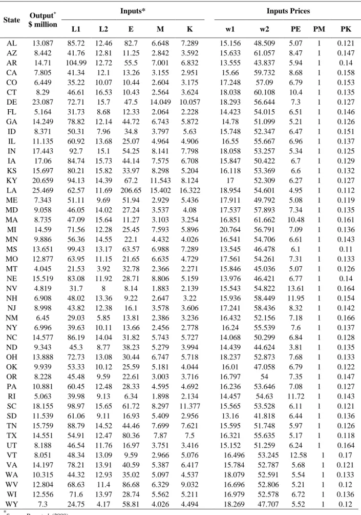
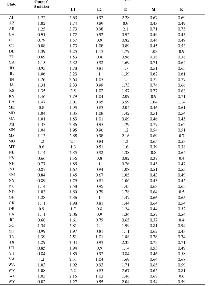
In this section, we consider the cost minimization of 48 states in the US. The data for this example is constructed from the 2002 Economic Census – Manufacturing for the USA (United States Census Bureau, 2002) used in Ray et al. (2008) for cost minimization choice of production location. Analogously to Ray et al. (2008) we assume one output which is measured by the gross value of production and five inputs including 1) Production labour (L1), 2) non-production labour (L2), 3) capital (K), 4) energy (E) and 5) materials (M). We also assumed that all prices are fixed as listed in Table 1 but input and output variables follow normal distribution with known mean and standard deviation that are given in Table 2 and Table 3.
- L1 is measured by the number of hours worked. The corresponding input price is wage paid per hour to production workers (w1). However, because different economy in different states, the input prices for production labour in different states are reported in the
19
column w1 in Table 1. For example, for Alabama (AL), the wage paid per hour is $15.156.
- L2 is the number of non-production employees and its corresponding wage rate (w2) is total emolument per employee (e.g. for Alabama, the hourly salary per non-production employee is $48).
- E is constructed by deflating the expenditure on purchased fuels and electricity by a state-specific energy price (e.g. for Alabama, the average energy price is 5.07).
- M is total expenditure on materials, parts, and containers is used as a measure of the materials input quantity, its input price assumed to be fixed (unity) for every state.
- K is the average of beginning and end of the year values of gross fixed assets and its corresponding input price is measured by the sum of depreciation, rent, and (imputed) interest expenses per dollar of gross value of capital (e.g. for Alabama, the average cost of capital (price of capital) is 0.121).
---Insert Table 1 here---
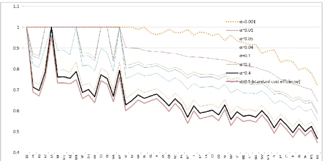
Table 3 presents the results of the stochastic cost efficiency model for the distinct -values. The value of represents the pre-determined minimum probability that each of the constraints of (11) fails to satisfy. If =0.05, then the five percentage of unsatisfied constraints is allowed by the decision maker. Since is a predetermined acceptable risk, it can be used as a planning purpose.
The last column for α=0.5 corresponds to the standard deterministic cost efficiency (Farrell cost efficiency), while other columns represent stochastic cost efficiency at given levels of α. Comparison of the Farrell cost efficiency results with chance-constrained cost efficiency results provides interesting insight. Overall the chance constrained scores for each DMU are higher than (or equal to) the deterministic counterparts. It is evident from the reported results that DMUs have a higher efficiency score under α=0.001 compared with other probability levels. This is also illustrated in Figure 1.
---Insert Table 3 and Figure 1 here---
Under all given probability levels, Delaware (DE) isthe best performer. Louisiana (LA) is stochastically efficient for 0.001 0.3but not Farrell cost efficient. Interestingly, Table 3 and Figure 1 show that efficiency increases when assuming lower probability, i.e.
20
Effα=0.001 ≥ Effα=0.01 ≥ Effα=0.04 ≥Effα=0.05 ≥ Effα=0.1 ≥ Effα=0.3 ≥ Effα=0.4 ≥ Effα=0.5.
Table 3 also shows that the number of stochastically cost efficient states increases as decreases. Only DE is stochastically cost efficient for = 0.5, equivalently Farrell cost efficient, while there are four and eighteen stochastically cost efficient states for =0.05 and
=0.001, respectively. Table 4 shows the benchmark units for each state. For stochastically cost inefficient states, DE is the only benchmark or contributes the obtained efficient target for every inefficient state. For =0.1 where DE and LA are stochastically cost efficient, the efficient targets of IN, ND, TX, WA and WI are formed by DE and LA.
For an illustrative purpose, suppose the state government of AL (Alabama), which tries to develop its cost-efficient state economy by maintaining the previous year’s output value, and its hypothetical economic planning department (division) is in charge. In order to develop a cost-efficient state economy for the next year, the department attempts to provide an efficient target. However, the next year’s overall economic situation is not certain and hence a practical production possibility set cannot be deterministic, i.e., the inputs and outputs of all states to be used to construct empirical technology sets representing various future production possibilities should be treated as stochastic. Now consider the situation where the economic planning department decides to use the stochastic cost efficiency criterion and then take the risk of =0.01 based on Tables 1-4 and other available economic information. Then the efficient target is obtained as the convex combination of DE and LA. The computation of (11) yields the following feasible optimal solution vector
* * * * *
7 16
, , , , 0.721798, 58.13526, 1.467466, 0.56954, 0.131606
p v u v
,
where the numbers 7 and 16 in the subscripts represent DE and LA, respectively. Considering the first constraint in (11) leads to the following relationship:
1 1 1 1 1 n m j ip ij j i p m m ip ip ip ip i i w x v w x w x
,21
48 48 * * 1 * 7 ,1 ,7 16 ,1 ,16 1 1 48 ,1 ,1 ,1 ,1 1 1 * 2119.675 2580.4736 2.3263 0.66376424 0.0580338 0.01 0.56954 0.131606 58.13526 2330.413429 2330.413429 4 i i i i i i m i i i i i i p w x w x v w x w x
where the number 1 in the subscript indicates AL. The efficient input target vector for =0.01 is obtained as
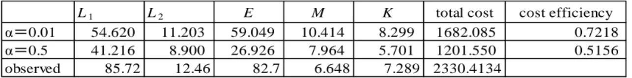
1 1 2 2 1 * * * 7 1,7 16 1,16 ,1 1 * * * * 1 7 2,7 16 2,16 ,1 * 2 1 * * * * 7 7 16 16 ,1 * 1 * * * * 7 7 16 16 ,1 1 * * * 7 7 16 16 ,1 0.01 0.01 0.01 0.01 0.01 L L L L E E M M K v L L c w v L L L c w L v E E E c w M v M M c K w v K K c w 54.620 11.203 59.049 10.414 8.299 K where 1 L c , 2 Lc , cE , cM and cK are observed cost shares. Note that the risk factor
1 1 * ,1 0.01 v /wL weighted by 1 L c is added to * * 7L1,7 16 1,16L in order to obtain the efficient target for the L1 input.Similarly, the other input targets are obtained. The total minimum cost for =0.01 is 1682.085 and the observed cost is $2330.413 million, in which case the stochastic cost efficiency is 0.7218. In contrast, for =0.5 the total cost is $1201.550 million with the cost efficiency of 0.5156 which is equivalent to the Farrell cost efficiency score. See Table 5. Rather than taking the risk of allowing for the 50% violation of each constraint in (11) to obtain the efficiency score of 0.5156, it is desirable to take a smaller risk of the 1% violation according to the proposed stochastic cost efficiency analysis. The stochastic cost efficiency method can aid policy makers with the economic planning decisions since we live in the world of uncertainty.
22
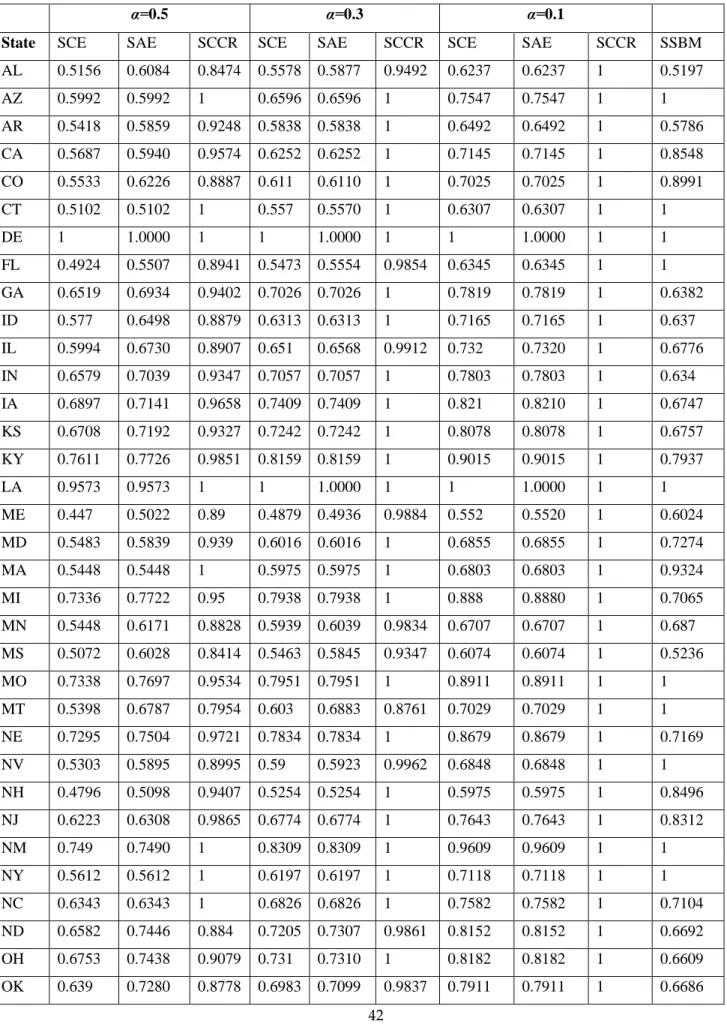
Before concluding this section, we provide an illustration based on the 2002 Economic Census that we utilise in this section.According to Table 6, Alabama represented by AL, which is used as our illustrative example, is the least efficient in terms of the stochastic SBM model with a score of 0.5197, while its target DMUs DE and LAare the most efficient with the score of one.For the stochastic decomposition analysis, we focus on α=0.5, 0.3 and 0.1 because some DMUs have a score more than one for α less than 0.1 (see Table 6). For all chosen α-values in Table 6, DE has always the best performance and LA is the best or the second best performance among all the states with respect to stochastic AE andstochastic CCR. This indicates that the early results of stochastic CE are consistent with those of stochastic AE and stochastic CCR. An additional important finding is that stochastic AE is less than stochastic CCR for all DMUs except for the stochastic cost efficient DMUs. This signposts that the allocative inefficiency arising from the wrong mix of inputs for given input prices, is more severe than the radial technical inefficiency.
---Insert Table 6 here---
We emphasize that the data used in this application and theanalysis does not aim to represent an in-depth or meticulous study of the problem at hand, but rather to show the applicability of our method. The key feature of the models in this study is that they enable managers to view more appropriate economic efficiency measures.
7. Concluding remarks and future work
Cost efficiency evaluates the ability of DMUs to produce the current outputs at minimal cost, given exogenous input prices. Analogously, revenue efficiency provides an estimate of attainable maximum revenue for a given input intensity and a set of output prices. In the conventional deterministic view of economic efficiency, the ex post evaluation is made for the case of deterministic and known prices. However, as many production and process planning decision are made in anticipation of unknown and stochastic information, the evaluation introduces a bias with unknown properties. Naturally, a parametric stochastic approach such as SFA may be used to address the stochastic nature of the composite variables cost and revenue, but resorting to a parametric approach introduces additional strong assumptions of the entire production set and the distribution of the inefficiency. This paper focuses at the case of stable and known deterministic market prices, exposed to random influences only through
23
the production technology. Such applications are readily found in e.g. financial intermediation, banking, utilities, food processing and logistics.
Precisely speaking, this paper has developed economic efficiency, both cost and revenue efficiencies, when input and/or output data of the DMUs are considered to be stochastic whereas input prices are known and deterministic. The chance-constrained program proposed in this study requires the known mean and variance, along with assuming the normal distribution for the input/output data of each unit. We show that the deterministic equivalent of the stochastic model, can be converted to a quadratic problem. The key parameter in the model is the chance constraint parameter alpha, also used in Charnes and Cooper (1959) and in the SDEA models (Land et al., 1993).
In the application on US state data, the findings show an interesting pattern when the stochastic model is applied. Whereas the deterministic model heavily penalizes the performance of certain states down to as much as 55% lower cost efficiency, the stochastic model shows broad ranges of states with comparable cost efficiency results in the ranges around 30-40% lower than best practice. Of course, the assumptions regarding the data generation process for the input prices in the application can be discussed, given regional patterns of population, unemployment and required skills. Nevertheless, we suspect that the distribution of the estimates from the stochastic model more closely mimics the true economic situation for a future decision than the deterministic frontier results. The decision maker must take into account not only the expected value for the input prices, but also their underlying variance, even in terms of the economic efficiency of the entities to be assessed.
Further work may concern the case of input and output prices that are stochastic. In addition, one may explore the determination of mean and variance and extending the model for non-standard normal distribution of data, for example, cases that data follows skewed or truncated normal distribution since in many real applications ‘sticky’ prices are primarily changing upwards.Since data in many real-world problems are relatively noisy, another future research direction would be to scrutinise the robustness of the results of the proposed model in this study in face of SFA.
References
Amirteimoori, A., Kordrostami S., Rezaitabar A., (2006). An improvement to the cost efficiency interval: a DEA-based approach. Applied Mathematics and Computation, 181, 775–81.
24
Bagherzadeh Valami, H., (2009). Cost efficiency with triangular fuzzy number input prices: An application of DEA, Chaos, Solitons and Fractals,42, 1631–1637.
Banker, R.D., Charnes, A., Cooper, W.W., (1984).Some method for estimating technical and scale inefficiencies in data envelopment analysis, Management Science, 30 (9) 1078–1092.
Battese, G.E., Coelli, T.J., (1992).Frontier production function, technical efficiency and panel data with application to paddy farmers in India.Journal of Productivity Analysis,3, 153-169.
Bjurek, H., Hjalmarsson, L., Førsund, F.R., (1990). Deterministic parametric and nonparametric estimating of efficiency in service production: A comparison, Journal of Econometrics, 46, 213-227.
Bruni, M.E., Conforti, D., Beraldi, P., Tundis E., (2009).Probabilistically constrained models for efficiency and dominance in DEA.International Journal of Production Economics, 117(1), 219–28. Camanho, A.S., Dyson, R.G., (2005). Cost efficiency measurement with price uncertainty: A DEA application to bank branch assessments. European Journal of Operational Research, 161, 432–446. Camanho, A.S., Dyson, R.G., (2008). A generalization of the Farrell cost efficiency measure
applicable to non-fully competitive settings. Omega, 36 (2008) 147–162.
Charnes, A., Cooper, W.W., (1959). Chance constrained programming. Management Science, 6, 73-79.
Charnes, A., Cooper, W.W., (1963). Deterministic equivalents for optimizing and satisfying under chance constraints.Operations Research, 11, 1 18-39.
Charnes, A., Cooper, W.W., Rhodes, E., (1978). Measuring the efficiency of decision making units,
European Journal of Operational Research, 2 (6), 429–444.
Coelli, T.J., (1996). Simulators and hypothesis tests for a stochastic model: a Monte Carlo analysis.
Journal of Productivity Analysis, 6, 247-268.
Cook, W.D., Seiford, L.M., (2009). Data envelopment analysis (DEA) - Thirty years on, European Journal of Operational Research, 192, 1-17.
Cooper, W. W., Tone, K., (1997). Measures of inefficiency in data envelopment analysis and stochastic frontier estimation.European Journal of Operational Research,99, 72-88.
Cooper, W.W, Huang, Z., Li, S.X., (1996). Satisfy DEA models under chance constraints. The Annals of Operations Research, 66, 279-295.
Cooper, W.W., Deng, H., Huang, Z., Li, S., (2002b). A chance constrained programming approach to congestion in stochastic data envelopment analysis. European Journal of Operational Research, 53, 1-10.
Cooper, W.W., Deng, H., Huang, Z., Li, S.X., (2002a). Chance constrained programming approaches to technical efficiencies and inefficiencies in stochastic data envelopment analysis. Journal of the Operational Research Society, 53, 1347–1356.
Cooper, W.W., Deng, H., Huang, Z., Li, S.X., (2004). Chance constrained programming approaches to congestion in stochastic data envelopment analysis, European Journal of Operational Research, 155, 487-501.
Cooper, W.W., Huang, Z.M., Lelas, V., Li, S.X., Olesen, O.B., (1998). Chance constrained programming formulations for stochastic characterizations of efficiency and dominance in DEA.Journal of Productivity Analysis, 9, 530–579.
Dempster, M.A.H., (1980). Stochastic Programming. Academic Press, London.
Emrouznejad, A. and De Witte, K. (2010). COOPER-framework: A unified process for non-parametric projects. European Journal of Operational Research, 207(3): 1573-1586
25
Emrouznejad, A., B. R. Parker, Tavares G. (2008). Evaluation of research in efficiency and productivity: A survey and analysis of the first 30 years of scholarly literature in DEA. Socio-Economic Planning Sciences 42(3): 151-157.
Fang, L., Li, H., (2012). A comment on “cost efficiency in data envelopment analysis with data uncertainty”.European Journal of Operational Research, 220, 588–90.
Fang, L., Li. H., (2013). Duality and efficiency computations in the cost efficiency model with price uncertainty. Computers & Operations Research, 40, 594–602.
Färe, R., Grosskopf, S., Lovell, C.A.K., (1985).The measurement of efficiency of production. Kluwer-Nijhoff Publishing: Boston.
Farrell, M. J., (1957). The measurement of productive efficiency.Journal of Royal Statistical Society, Series A, 120, 253–281.
Huang, Z., Li, S.X., (1996). Dominance stochastic models in data envelopment analysis.European Journal of Operational Research, 95 (2), 390–403.
Jahanshahloo, G. R., Soleimani-damaneh, M., Mostafaee, A., (2008). A Simplified version of the DEA cost efficiency model. European Journal of Operational Research, 184, 814–815.
Kall, P., Wallace, S. W., (1994). Stochastic Programming.John Wiley & Sons.
Kuosmanen, T., Post, T., (2001). Measuring economic efficiency with incomplete price information: With an application to European commercial banks, European Journal of Operational Research,134, 43–58.
Kuosmanen, T., Post, T., (2002). Nonparametric efficiency analysis under price uncertainty: A first-order stochastic dominance approach, Journal of Productivity Analysis, 17 (3), 183–200.
Kuosmanen, T., Post, T., (2003). Measuring economic efficiency with incomplete price information,
European Journal of Operational Research, 144, 454–457.
Lahdelma, R., Hokkanen, J., Salminen, P., (1998). SMAA––stochastic multiobjective acceptability analysis, European Journal of Operational Research, 106, 137–143.
Lahdelma, R., Salminen, P., (2001). SMAA-2: Stochastic multicriteria acceptability analysis for group decision making, Operations Research, 49 (3), 444–454.
Lahdelma, R., Salminen, P., (2006). Stochastic multicriteria acceptability analysis using the data envelopment model.European Journal of Operational Research 170, 241–252.
Land, K. C., Lovell, C. A. K., Thore, S. (1993).Chance constrained data envelopment analysis.
Managerial and Decision Economics, 14, 541–554.
Liu, B. (1997). Dependent-chance programming: A class of stochastic programming. Computers &Mathematics with Applications, 34(12), 89–104.
Liu, B. (1999). Uncertain programming. New York: John Wiley & Sons.
Liu, J.S., Lu, L.Y.Y., Lu, W.M., Lin, B.J.Y. (2013) A survey of DEA applications, OMEGA 41(5): 893–902.
Luenberger, D.G. (1995). Microeconomic Theory.McGraw-Hill, Boston.
Morita, H., Seiford, L. M. (1999). Characteristics on stochastic DEA efficiency.Journal of Operational Research Society of Japan, 42(4), 389–404.
Mostafaee, A., Saljooghi, F.H., (2010). Cost efficiency measures in data envelopment analysis with data uncertainty. European Journal of Operational Research, 202, 595–603.
Olesen, O.B., (2006). Comparing and combining two approaches for chance constrained DEA.
26
Olesen, O.B., Petersen, N.C., (1995). Chance constrained efficiency evaluation. Management Science, 41, 442–457.
Olesen, O.B., Petersen, N.C., (2015).Stochastic Data Envelopment Analysis - A review.European Journal of Operational Research, In Press.
Ray S. C., Chen L., Mukherjee L. (2008). Input price variation across locations and a generalized measure of cost efficiency, International Journal of Production Economics, 116 (2), 208–218 Schafinit, C., Rosen, D., Paradi, J.C., (1997). Best practice analysis of bank branches: An application
of DEA in a large Canadian bank. European Journal of Operational Research, 98, 269–289. Simon, H. A. (1957). Models of man. New York: John Wiley and Sons, Inc.
Sueyoshi T., (2000). Stochastic DEA for restructure strategy: an application to a Japanese petroleum company. Omega, 28(4), 385–98.
Talluri, S., Narasimhana, R., Nairb, A., (2006). Vendor performance with supply risk: a chance-constrained DEA approach. International Journal of Production Economics, 100, 212–222.
Tavana, M., Khanjani Shiraz, R., Hatami-Marbini, A., Agrell, P., Paryab, K., (2012).Fuzzy stochastic data envelopment analysis with application to Base Realignment and Closure (BRAC).Expert Systems with Applications, 39 (15), 12247-12259.
Tavana, M., Khanjani Shiraz, R., Hatami-Marbini, A., Agrell, P., Paryab, K. (2013). Chance-constrained DEA models with random fuzzy inputs and outputs. Knowledge-Based Systems, 52, 32–52.
Tavana, M., Khanjani Shiraz, R., Hatami-Marbini, A. (2014).A new chance-constrained DEA model with birandom input and output data.Journal of the operational research society, 65, 1824–1839. Thompson, R.G., Dharmapala, P.S., Humphrey, D.B., Taylor, W.M., Thrall, R.M., (1996). Computing
DEA/AR efficiency and profit ratio measures with an illustrative bank application.Annals of Operations Research, 68, 303–327.
Tsionas, E.G., Papadakis ,E.N., (2010). A Bayesian approach to statistical inference in stochastic DEA.Omega, 38, 309–314.
Udhayakumar, A., Charles, V., Kumar, M., (2011).Stochastic simulation based genetic algorithm for chance constrained data envelopment analysis problems, Omega, 39, 387–397.
Wu, D., Lee, C.G., (2010). Stochastic DEA with ordinal data applied to a multi-attribute pricing problem. European Journal of Operational Research, 207, 1679–1688.