Predicting fault-prone software modules with rank sum classification

Predicting Fault-Prone Software Modules with Rank

Sum Classification

Jaspar Cahill, James M. Hogan and Richard Thomas School of EECS, Faculty of Science and Engineering

Queensland University of Technology Brisbane, Australia

[email protected], {j.hogan,r.thomas}@qut.edu.au

Abstract—The detection and correction of defects remains among the most time consuming and expensive aspects of software development. Extensive automated testing and code inspections may mitigate their effect, but some code fragments are necessarily more likely to be faulty than others, and automated identification of fault prone modules helps to focus testing and inspections, thus limiting wasted effort and potentially improving detection rates. However, software metrics data is often extremely noisy, with enormous imbalances in the size of the positive and negative classes. In this work, we present a new approach to predictive modelling of fault proneness in software modules, introducing a new feature representation to overcome some of these issues. This rank sumrepresentation offers improved or at worst comparable performance to earlier approaches for standard data sets, and readily allows the user to choose an appropriate trade-off between precision and recall to optimise inspection effort to suit different testing environments. The method is evaluated using the NASA Metrics Data Program (MDP) data sets, and performance is compared with existing studies based on the Support Vector Machine (SVM) and Naïve Bayes (NB) Classifiers, and with our own comprehensive evaluation of these methods.

Keywords— Metrics, fault proneness, machine learning I. INTRODUCTION

Software development has progressed considerably since its beginnings half a century ago, yet software maintenance and testing still account for a substantial proportion of total development cost [1]. Testing and code inspections have increased in sophistication, and the rise of automated testing frameworks has allowed far greater coverage for equivalent cost than in the past. Yet the development of tests and the practice of code inspections remain a significant overhead, and there are powerful arguments that support a focus of this effort on classes and packages that carry greater risk of defects than others. The problem is then to identify such modules reliably and automatically, thus making a more intensive local effort worthwhile. Some ad hoc or rule of thumb approaches are possible, but in this paper we adopt a more data-driven approach, using machine learning methods to develop predictive models of fault proneness [2].

The fundamental idea is that software modules may be described adequately by software metrics – rapidly collected using automated tools – which may then be related to defect counts obtained for each module during testing and production. Each module is thus viewed as an ordered pair (,), where

is the vector of metrics scores, and is the associated label, either FAULTY or NOT_FAULTY, although these are usually captured by the numeric values {+1, −1}. We then use machine learning algorithms to establish a mapping between the module data vectors and fault proneness, often making these inferences without extensive reliance on low level domain knowledge. Indeed, we make the assumption that the metrics collected may capture structural information as reliably as a domain expert, an assumption supported by results of earlier modelling efforts, and made more attractive through the obvious advantages in speed and cost [3,4].

A number different machine learning techniques have been applied to the problem of modelling fault proneness, and we here focus on those that used the data sets from NASA’s Metrics Data Program (MDP) [5]. The techniques used in these studies include for example, Random Forests [6], the Support Vector Machine (SVM) [3, 7], the Artificial Immune Recognition System [8], Expectation Maximisation [9], and Radial Basis Function networks [10]. Other earlier studies are cited in [2]. A recent paper systematically applied as many as 22 distinct classifiers to 10 of the NASA data sets, with the authors observing no significant difference in performance among the top 17 approaches [11]. One conclusion that maybe drawn from this work is that no stand-out classifier exists for fault proneness prediction, at least when based on traditional feature representations. More particularly, we observe that simple classifiers such as Naïve Bayes (NB) may work just as well as more sophisticated ones. The question is whether there remains additional information in the data set that might be exploited to improve performance. While this is still an open question, and one to which we make some contribution through the present study, there is a view that a performance ceiling has been reached, and that the way forward lies in enriching the data with new information beyond existing metrics [12]. Nevertheless, the NASA data sets are freely available and remain attractive targets for researchers.

In this study, an enhancement is proposed to improve the utility of predictive models for software managers, allowing some performance improvements and a more accessible trade-off between precision and recall. Such configurability is desirable in order to take account of the cost of inspection and the risk of undetected faults slipping into production. In systems for which there is a low tolerance of faults, a higher detection rate (TPR) may be sought at the expense of a higher false alarm 2013 22nd Australian Conference on Software Engineering

rate (FPR). For systems where testing budget is limited, a lower false alarm rate may be preferred.

Underlying our approach is a new representation, which we term‘rank sum’, in which a ranking abstraction is laid over bin densities for each class, and a prediction is determined based on the sum of ranks over features. A key part of the trade-off is provided by the output from this method, the rank sums for each class. This converts instance points into a bounded 2D ‘rank sum space’ where classes are better separated, and the trade-off readily visualised by the non-specialist. Applying the Support Vector Machine (SVM) algorithm to this 2D data provides the decision boundary, maximising the separation of the rank classes.

Rank sum is not applied naively over the entire feature set; rather, we performed an extensive Exploratory Data Analysis for the available data sets, and then applied a variety of standard feature selection and modelling approaches, with the optimal sets considered in a later section. These reduced feature vectors were used for baseline SVM and NB models, and as input to Rank Sum. Additionally, we used the well-established models from Menzies et. al. [13] as a benchmark, although there are variations in class definition from the present work.

This paper is organised as follows: section II provides some background information, largely on the data and our approach to feature selection. Application of the SVM and NB algorithms to generate baseline models is then described in section III. Attention then turns to the novel work of the rank sum classification method in section IV. Experiments on the NASA data show how its performance compares to the benchmark classifiers. Rank sum data is then used in section V with an SVM classifier to create trade-off specifiable models. The paper concludes in section VI with discussion of these results and future directions for research.

II. METRICS, DATA SETS AND FEATURE SELECTION

Automated modelling of software quality is critically dependent on software measurement, usually through an agreed set of scoring functions known as metrics. It is through quantitative metrics that software modules are described and in some useful sense summarised. These scores serve as the input in the mapping to be learnt between software module description and class label. The metrics of interest here are static code measurements, usually counts of some elements in the source code, reflecting structure and complexity. These are used because the availability of metrics tools means they are easily collected, and static metrics can be collected early in the software lifecycle.

The data sets used in this work are largely comprised of these static source code metrics, sourced from NASA’s Metrics Data Program. A number are based on or closely related to Lines of Code (LOC), while others comprise measurements from two common suites of metrics, those due to Halstead and McCabe. The Halstead metrics are based on Halstead's Software Science [14], a theoretical framework developed in the 1970's. Halstead metrics primarily measure program size and complexity, with examples including Volume, Error Estimate and Program Level. McCabe metrics measure structural complexity through

an abstract representation of the module as a control flow graph. The best known of these metrics is Cyclomatic Complexity [15]. The nature – or indeed the potential absence – of the relation between these metrics and fault proneness is an obvious limitation on the value of this work. However, earlier studies [3, 4] have delivered models derived from the NASA metrics which perform at a level comparable with manual code inspection. Whatever their limitations, the metrics data do not preclude the development of useful models. These studies also show that the metrics produce better performing models than ones based on LOC alone. It might be mentioned nevertheless, that a marked relationship between complexity as measured by CC and fault count was found in [16].

Altogether there are 9 data sets, each derived from a different software system, with example systems including ground or satellite control systems. All systems were implemented in the C language, except for sets kc1 and kc3, which were implemented in C++ and Java respectively. The unit on which metrics are collected is the function, also referred to here as a module or instance. The number of metrics given for each module is 43, the exception to this being jm1andkc1, which have about half the number of features reported for the other sets. The number of modules in each data set varies considerably. Most are in the range 400 to 2100 with the exception of two larger sets, pc2 and jm1, which have 5589 and 10878 modules respectively.

An important metric also included in each data set is the fault count for each module, and we will use this count to establish the true binary class label. Across all data sets, the average percentage of modules with at least one fault is 10%, which, while low, may reflect some of the inevitable compromises in inspection and testing effort. Nevertheless, even the generous assumption that all of these modules should be regarded as FAULT_PRONE leads to massive class imbalance, and trouble for learning algorithms [17]. Moreover, the count based approach is flawed, taking no account of module size. While our approach has the effect of further reducing the size of the positive class, some normalisation is essential, and we rely upon afault density, the number of faults recorded per 1000 lines of code. Inspection of the fault density distribution allows an informed choice of threshold for labelling: we have chosen a fault proneness threshold of 40 faults per thousand LOC. This is typically just after the peak of log-normal error density distributions but still includes a substantial proportion of faulty modules. The choice is independent of performance curve that can be derived by varying the threshold. As noted, some variations make comparison between authors potentially difficult. Our choice is geared to a focus on ‘difficult’ modules, concentrating effort where it is likely to bear fruit. Modules with a fault density in excess of this figure are labelled as FAULT_PRONE; those below this threshold form the negative class.

As for any real world data, the NASA data sets are contaminated by noise [18, 19], though this has not been a central focus until recently [20]. The problem is most pronounced in jm1, the largest NASA data set; others are substantially less affected. For this reason, and others including a robustness to noise of the learners used in this study, the

difficulty there can be in distinguishing between noise and legitimate outliers in the population, and there being a preference to leave the data in as close to its real world form as possible, this type of noise was not removed. Recently though, attention has been drawn to a more significant issue of duplicate instances [20], potentially causing overlap between training and test sets and thus biased performance estimates. Though the severity of this effect has not yet been fully evaluated, it is likely to be less at least for the Naive Bayes classifier used here due to its robustness to duplicates.

Feature selection is an essential preparatory step if classifier performance is to be optimised [21], the objective being to find a subset of relevant features that capture the underlying structure of the data, without including irrelevant or redundant components [22]. In practice, in the supervised learning case, the objective is to find features that are correlated with or predictive of the class label [21].

There are two types of algorithm for selecting optimal feature subsets, the filter and wrapper [23, 24]. The filter approach filters out undesirable features prior to training. It involves a search through feature subset space, in which each subset’s merit is evaluated by a heuristic function. Ranking methods, distinct from subset methods, are simple filters that only evaluate the merit of each feature individually with respect to the class. The wrapper approach differs in that the subset evaluation function wraps a learning algorithm whose performance determines the merit of the subset.

Menzies et. al. [13] employed Information Gain (IG) based ranking for his benchmark study on the NASA data sets. While he found that this selection performed as well as two subset methods, in general the approach may lead to some redundancy in the set. Ranking methods are essential in the face of massive feature set size, but here the number of features is more modest, and there are few barriers to the use of subset and wrapper methods. Wrapper methods are the preferred option for best classifier performance, with an efficient search algorithm chosen to reduce processing time (the learning algorithm being invoked on each subset evaluation) and to avoid over-fitting, and our experiments are described in the following section. However, subset methods might also be considered as subset evaluations are relatively quick, and have the advantage of being generic and not affected by any particular algorithmic bias.

III. NAÏVE BAYES AND SUPPORT VECTOR MACHINE

In this section we apply Naïve Bayes (NB) and Support Vector Machine (SVM) classifiers to the NASA data sets, providing a comprehensive assessment of these methods over a very large selection of feature sets and model parameters, a near exhaustive exploration of the alternatives. These models serve as a baseline for the rank sum method described in later sections, and as a further contribution to the work begun by Menzies and others, our results supporting the view that there is little further to be gained from standard approaches. Feature sets extracted as part of this work are, however, a useful dimension reduction leading into the rank sum approach.

2_{The protocol requires application of 10-fold cross validation during learning,} with ten repeats of this process using a different random number generator seed for fold selection. The result reported is the mean over these runs.

The machine learning tool Weka [25] was used for both feature selection and learning. Following Menzies et. al. [13], we also consider an alternative, log-normalised version of the feature set, which he found to improve significantly the performance of the NB models. These feature sets are referred to as the normal and log normalised strands respectively.

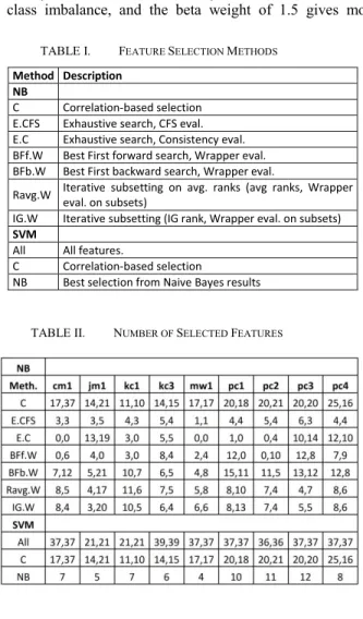
The feature selection methods employed are listed along with their abbreviated names in Table I. Some additional selection methods were used for NB as it is markedly quicker to train than the SVM. Feature selection is held to be less critical for the SVM, the method being more tolerant of a higher dimensional feature space and redundant features. A baseline is provided by the correlation selection method, ‘C’, in which features were selected simply by removing redundant features with a Pearson correlation coefficient exceeding 0.9, without preference to preserving one correlated feature over another. By these feature selection methods, resulting feature subset sizes are shown in Table II, the latter number in the pairs being for log normalised data, and in the last row the number is the size of the best subset found with NB, log normalised or not.

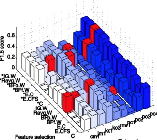
Naïve Bayes classifiers were learnt from each feature-selected data set under a standard 10 x 10 fold cross validation experimental protocol2_{. Results are shown in Figure I. The}

performance measure indicated is the F1.5 score, chosen because it allows performance to be measured as a single number (rather than TP and FP rates). The measure is sensitive to class imbalance, and the beta weight of 1.5 gives more

TABLE I. FEATURE SELECTION METHODS

Method Description NB

C Correlation-based selection E.CFS Exhaustive search, CFS eval. E.C Exhaustive search, Consistency eval. BFf.W Best First forward search, Wrapper eval. BFb.W Best First backward search, Wrapper eval.

Ravg.W Iterative subsetting on avg. ranks (avg ranks, Wrapper eval. on subsets)

IG.W Iterative subsetting (IG rank, Wrapper eval. on subsets) SVM

All All features.

C Correlation-based selection

NB Best selection from Naive Bayes results

importance to recall than precision, lessening the penalty on higher FP rates, which we tolerate more readily than detection failures. Feature sets obtained for the log normalised data are indicated with an asterisk preceding the method name. Best performance for each data set is indicated in red. It will be noticed from the figure that performance between data sets varies considerably. Log normalisation performs better only for some data sets, and generally does not appear to provide much benefit on this data – although this variation from the Menzies study may be due to the higher error density threshold applied. The results are not especially sensitive to the feature selection method, but the best, with a consistent edge over the others, is BFb.W. This is not a surprising result as wrapper methods tend to maximize classification performance.

The Support Vector Machine (SVM) is a discriminative model based on the Statistical Learning Theory of Vapnik [26] and complements the probabilistic approach of NB. A distinguishing feature is its ability to automatically find the optimal balance between model capacity and training set error

to maximise generalisation performance. The SVM approach employed here has two parameters, a cost penalty C, and the kernel selection, which itself may introduce additional parameters. A lower value of C permits some misclassification, in which points lie on the wrong side of the separating hyperplane, while a higher value forces the creation of a more accurate model of the training data that may not generalise as well. The kernel may map the original data into a higher dimensional feature space, providing for various types of non-linear decision boundaries. Models were created over a range of C values [10000, 100, 10, 5, 1, 0.5, 0.05]. Three standard kernels were also tried, Linear, Quadratic and the Radial Basis Function (RBF). The first two tended to classify all instances as negative for most data sets, so are not considered any further. RBF has a single parameter γ. Based on other studies [27, 28] 9 values were selected for this parameter [0.05, 0.1, 0.2, 0.3, 0.5, 0.7, 1, 1.5, 3]. Fivefold CV was used to obtain model performance for each parameter pair (C, γ). The total number of SVM models generated with this kernel was thus 9 data sets * 5 feature selections * 7 C values * 9 γ values * 5 CV = 14,175 models. These were run in parallel on multiple computers through Matlab.

Example results for the data set pc3 are shown in Figure 2. Segments of the plot are colour-coded by feature selection: All, *All, C, *C, NB. It will be noticed that many models performed poorly. Feature selection does not affect performance much, although larger feature sets tended to perform better, and surprisingly, better than the smaller selections that gave best performance with NB. Hard margins usually gave better performance than soft.

Performance of the two algorithms is compared in Table III. It will be noted that SVM was not able to find a model that could discriminate for jm1. For most data sets SVM performance was approximately 5% better than NB. In two cases there was a large difference, with SVM being ~20% ahead for pc1, and NB being 20% ahead for kc1. An interesting pattern in the results is that the false alarm rates for SVM are very low, particularly compared to some of those for NB. This is due to SVM’s tendency when classes are imbalanced to position the decision boundary close to the positives rather than an ideal position of some distance away from the positives. This results in fewer positive classifications, and correspondingly fewer false alarms.

Fig. 1. Naive Bayes results as F-score measures across (data set × feature selection method), with highest score for each data set

highlighted red.

Fig. 2. SVM results for data set pc3 as F-score measures over (7 C values × 9 lambda values × 5 colour-coded feature selections).

The hard margin tends to give better results in the imbalanced case as softening gives more importance to margin maximisation than penalisation of error (particularly positive error) and this tends to result in a large margin in which most instances are classified negative [29].

Results shown here are down from the earlier benchmark study of Menzies et. al. [13], but these differences are consistent with the additional class imbalance imposed by the different assignment of class labels, a problem especially pronounced for some data sets. Notwithstanding these changes, and the resulting difficulties for the learning algorithms, there are only modest differences for the best performed models, with F1.5 scores of 58 (the present work) and 60 (Menzies) for pc4, with 38 and 39 for kc3. These models serve well as a baseline for the studies of following sections.

IV. RANK SUM CLASSIFICATION

The rank sum method came about from observing the class probability plots for individual features. An example of class probabilities for a single feature is shown in Figure 3, the x-axis representing feature value range and the y-axis, value probability, with a separate curve for each class. Across features, for a given instance vector to be classified, the component values of the vector are positioned at different points along the x-axis of the density plots. For some features the component value will lie close to a peak (of a class), for others less so. The idea behind this method is that the more consistently component values lie closer to peaks across features for a given class, the more likely it is that the instance belongs to that class. Proximity to peaks is encoded using a ranking abstraction over the density curves.

The method is described formally in the next section, after which we consider an extension in which bin width is adjusted based on the distribution gradient. Experiments are then performed to evaluate the performance of the method.

A. Method

The method is intended to address the binary supervised learning problem, in which a function is to be learnt

}

1

,

0

{

)

(

x

o

f

From the training data, it is possible to describe a probability distribution for each class for each feature. These distributions are discretised by partitioning the range of the feature into bins, at this point of equal width – the range of the feature divided by the number of bins. For each bin a probability is calculated relative to each class rather than to the total number of instances in the training data. For an attribute value , the bin probability for bin given class C, is calculated as:

= =#(∈ ) ^(_#{ ∈ ) ∈ } ,

(1)

the fraction of the values of the class that lie in Bj.

The scenario may be visualised by considering two dice, one for each of the labelled classes. The sides of each die correspond to bin numbers, and each has probability . In rolling the dice, because they are biased, the sides with the larger probabilities will occur more often. For the purpose of trying to determine the true underlying class which generated the outcomes, it is more convenient if the outcomes are sorted according to probability. Thus, if the outcome from one of the dice is 1, in the absence of a similar outcome from the other die it is likely that the example is of the former class. The sorting of sides or bins according to probability effectively imposes a rank ordering, B’:

∈ = , ℎ ≥ ≥ … ≥ (2)

TABLE III. NBAND SVM RESULTS

NB SVM Best sel. #Sel. TPR FPR F1.5 Best sel. #Sel. C γ TPR FPR F1.5 Win cm1 BFb.W 7 38 8 29 *All 37 100 1 30 3 31 SVM (3%) jm1 BFb.W 5 74 50 26 NB kc1 *BFb.W 7 72 38 28 *All 21 100 3 6 1 8 NB (20%) kc3 BFb.W 6 47 10 38 All 39 10000 0.05 44 5 43 SVM (5%) mw1 BFf.W 2 25 1 27 C 17 10000 0.05 25 2 23 NB (4%) pc1 *Ravg.W 10 34 8 25 All 37 10000 0.3 47 4 44 SVM (19%) pc2 BFb.W 11 43 4 9 *All 36 10000 0.2 13 0 14 SVM (5%) pc3 BFf.W 12 37 11 28 *All 37 10000 1.5 37 6 35 SVM (7%) pc4 *BFb.W 8 95 24 54 *All 37 10000 0.3 58 5 56 SVM (2%)

Fig. 3. Class probability distributions for an exemplar feature, the curves based on feature values for each class.

B’1 then has probability b1 which is the largest bin

probability for that class. Throwing a die for each feature leads to a multinomial distribution over the ranked bins 1..n, where the probability of each ‘face’ is bj.

For the purpose of classifying an instance, a rank function is defined which gives the rank for particular value xi of a feature,

() = ′ (3)

The rank sum for a given class for instance vector x is then given by:

!"$%& = ' ()

*

(4)

The predicted class is that corresponding to the larger rank sum.

B. Method Modification: Gradient Binning

A problem found with the method as described is that ranks for each class for a given feature (as distinct from rank sums) were often the same, or very similar, at or near the highest rank, leading to similar rank sums across classes and hampering classification. To some extent this cannot be avoided as most points will lie in the bins with highest rank. But the problem may be exacerbated by the fact that even though the probability may change dramatically on the peak between two values within a bin, the rank would still be considered the same, even though with such a change it could be reasonable to expect a drop in rank. At the opposite extreme, varying ranks may be assigned to nearby bins even if the curve over these bins is essentially flat. The solution to the problems is to tie bin width to the gradient of the probability distribution, adaptively selecting narrow bins when the curve changes significantly, and merging bins where the curve changes little. Bins are created by first forming the distribution curve from a specified number of bins. Then, horizontal lines are run across the distribution curve. They are spaced vertically across the y-axis range at an equal width apart, according to a specified number of ‘density levels’. Points of intersection between these lines and the curve are projected onto the x-axis, to form bin edges. An additional minimum bin width parameter (as a proportion of the feature range) provides a limit to how narrow the bins can be. Following this procedure, bin probabilities are recalculated to reflect the new widths.

Some exploration of these approaches showed that instances with greater rank difference were classified more accurately, and also that gradient binning was effective in increasing the average rank difference – although this latter effect was not dramatic. Though a tailored distribution partitioning method has been used here, that used in standard discretisation methods, such as ChiSplit based on the chi-square statistic [30], could be explored.

C. Modelling Experiments

Experimental results using rank sum are considered below. Initial work investigated the effect of optimal selection of bin parameters for each individual feature – an approach logical

given the dependence of classification on the summation of the individual ranks. Optimal bin parameters were found for each feature, and then two features with these parameters were modelled in combination to see if performance could be improved. The four features chosen were those selected by the CFS feature selection algorithm on the pc4 data set, lCp, lCC, dP and mMS (percent comments, code and comments, parameter count, maintenance severity). Optimal parameters for each feature were found by obtaining model performance with cross validation on different parameter combinations over both classes, with number of bins ranging from 30 to 170 by 20, and a wide range of density levels [2 3 5 7 10 20 30 50]. Minimum bin width was fixed at 0.005, so as not to override the original gradient derived bins. Optimal parameters for each feature were selected according to the best-performed model. Results for each feature are shown in Table IV. For each feature, best performance was obtained with the values shown for the bin parameters b and d for each class, which correspond to number of bins, and number of density levels respectively. It will be noticed that ‘density levels’ is quite low in some cases, as low as 2 which makes for a very coarse ranking. Also, the parameters for the negative class only approximately match those of the positive class for 2 of the 4 features, which might suggest that bin parameters should be class specific.

Some additional experiments were conducted to exploit combinations of features, the most successful involving a best first search of subsets based on a ranking of features according to individual performance. The same approach was repeated with the data set, kc3. Results for both data sets are shown in Table V, including the abbreviated names of features selected, with NB performance from Table III shown for comparison. The performances between the methods are virtually identical by the F1.5 score – raw rank sum performs as well as NB on the NASA data. Lower TP rates might be due to the use of the F1 measure in model selection rather than F1.5. Feature selections also differ markedly between the approaches.

While these initial performance results were encouraging, they were obtained with substantial and rather complex exploration of the bin parameters, making the approach less than practicable. Applying similar parameter settings to all features greatly simplifies model selection, with minimal loss in performance: for pc4, a result only 2% less than the best

TABLE IV. INDIVIDUALLY OPTIMAL PARAMETER SELECTIONS

Neg Pos Performance

b d b d TP FP F

lCp 60 30 60 20 79 32 31 lCC 30 30 60 2 76 19 41 dP 30 3 45 3 70 52 20 mMS 90 3 30 30 95 86 18

TABLE V. COMPARISON OF RSAND NB RESULTS

Data Meth. Features TPR FRP F1.5 pc4 RS lCC, mEd, mVe, lB, dP, cCP, mMS 69 11 55 NB lB,lCC,mIv,mVe,dP,gCmod,mVn,lCp 95 24 54 kc3 RS mVd, mGd, mEd, lCC, mVe, hD, mMS 50 11 38 NB lCC,mGd,hD,hL,mMS,lCp 47 10 38

performance of 55 was obtained using 30 and 110 bins for negative and positive classes respectively, and corresponding density levels of 10 and 5. A similar near optimal result was obtained for kc3, using bin numbers 30 and 60 and density levels 2 and 30.

V. TRADE-OFF MODELS

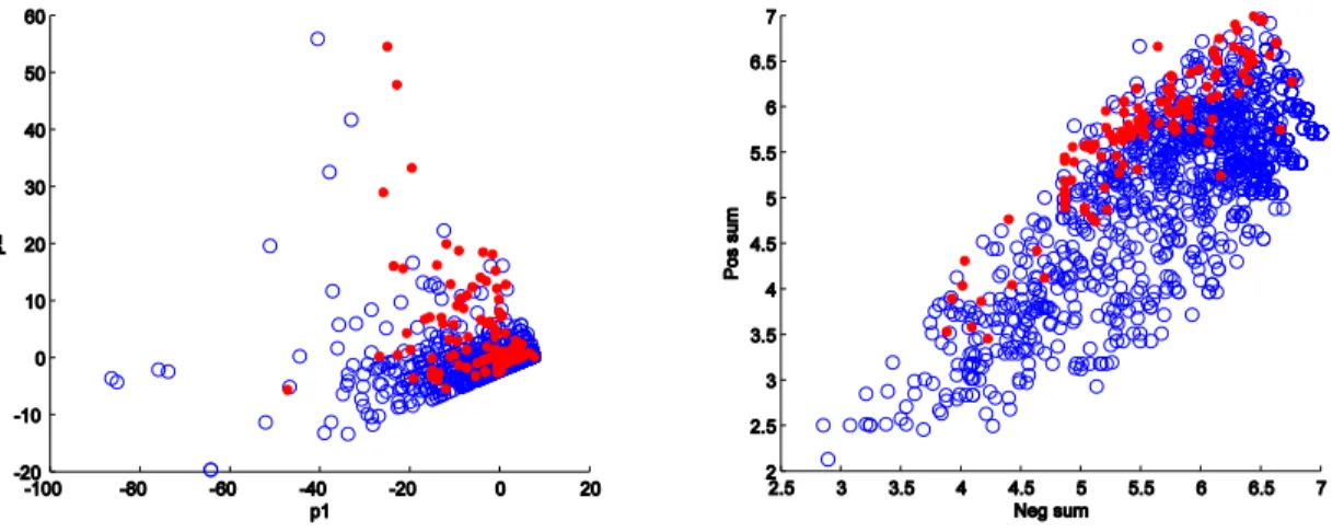
While rank sum may be used directly, with classification based on the class with the greater value, better results may be achieved through a more sophisticated approach to the placement of the decision boundary. Rank sum provides an effective low dimensional encoding of the class information – with notably superior separation when compared with PCA (Figure 4)– but some noise remains. Use of a robust classifier such as the SVM on this data allows us to optimise the trade-off between precision and recall, and to make the selection explicit in the configuration of the problem. Here we focus on the pc4 data set, being the best performing of the NASA data sets, although results are also given for kc3. Results with two kernels are described, linear and RBF.

The SVM experiments described in this section were performed using the Spider Machine Learning toolbox for Matlab (The Spider), which relies on the well-known LIBSVM library. A modified display function from this library produced the SVM illustrations that follow.

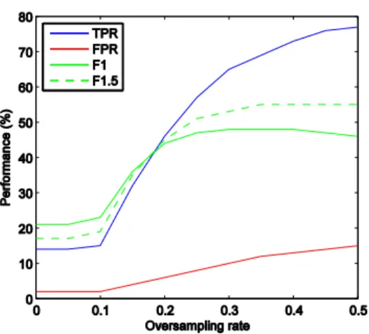
Notwithstanding the more effective class separation provided by rank sum, the problem of class imbalance remains and is here handled through the use of random oversampling of the positive class. The oversampling experiment with the linear kernel was straightforward. The C value was set to a hard margin, as this gave the best result without oversampling, and oversampling was applied to the positives at increasing levels from 0% to 100%. The oversampling percentage of positives is relative to the size of the negative class, so at 50%, there are half as many positives as negative, and at 100% the classes are balanced. Tabulated results are not shown for all of these experiments, but performance dramatically improves with an oversampling level above 50%. This can be seen clearly in a

plot of the decision boundary shown in Figure 5, which appears to be well placed in separating the classes, while illustrating the inevitable problem of false positives intermingled with the correctly labelled instances. The F1.5 score here is 55, comparable to the very best performance from other algorithms and previous studies. The oversampling rate provides control of the model, allowing us to choose the desired trade-off between detection and false alarms, and the trade-off curve is obtained by varying the oversampling level from 0 to 50% at increments of 5% (Figure 6).

Oversampling proved beneficial only for soft margin RBF classifiers, but provided no improvements over the linear kernel. Figure 7 shows the results of an experimental run with an oversampling rate of 30% with C at 10 and γ at 0.4. The left figure shows the result without oversampling, and the right is the result with oversampling. The additional oversampling parameter – coupled with the existing γ and C values - led to a three dimensional matrix of parameters for RBF model

Fig. 4. Scatter plot of PCA-transformed pc4 with fault prone modules shown in red on the left, and right, by comparison, the same data set transformed with rank sum showing improved class separation.

Fig. 5. SVM linear decision boundary between fault prone and not fault prone modules, on rank sum transformed pc4 with oversampled positives.

selection, with experiments following a similar protocol to those described above. The best results were obtained with γ = 0.4, as shown in Table VI. Optimal performance is seen in the bottom row, with an F1.5 score of 51. A trade-off effect is evident in most of the columns of the table as oversampling level is varied.

For kc3, the linear kernel with oversampling also produced the best result, in this case with hard margin and an oversampling level of 35%. The trade-off curve is again obtained by varying the oversampling level. As for pc4, the best result was comparable with the other learning algorithms while also allowing a desired trade-off point.

VI. CONCLUSIONS

In this paper we have considered again the problem of predicting fault prone software modules based on a set of metrics collected over the codebase. The work differs from some earlier studies in its focus on difficult modules – with class labels chosen to reflect non-trivial fault densities rather than the occurrence of a single defect. This changes the nature of the problem, eliminating noise from examples of very low fault density, but exacerbating the already troublesome issue of class imbalance. Traditional feature representations and classification approaches – seen here in the near exhaustive exploration of SVM and NB models for the problem – suggest that the problem

is more difficult than the simpler labelling employed by other authors, though some useful models did emerge from this process.

Analysis of these results lends support to the view of Menzies et. al. [12] that a performance ceiling has been reached in exploiting metrics data of this type using traditional approaches, and we note the limited variation seen across our models for a very wide range of parameter settings and feature sets. The low F scores highlight the difficulty in correctly labelling fault prone modules without paying an enormous penalty in false positives. The major contributions of this paper go to the heart of these problems, by introducing a new feature encoding to improve class separation and using oversampling as a means of addressing the class imbalance, and ultimately to control the trade-off between the TPR and the FPR.

Simple rank sum classification – the prediction being given by the larger class-specific rank sum – offers performance comparable to NB with a similar level of effort. More importantly, the low dimensional encoding of the data via rank sum provides near optimal separation of the classes, and allows clear visualisation of the data set and the trade-offs inherent in prediction. Oversampling may be used to correct for class imbalance and to make gradual adjustment of the decision surface in accord with the requirements of the user, generally accepting a modest false positive rate in return for improvements in recall.

Predictive models of fault proneness in software modules seem unlikely to advance much further without a substantial re-assessment of the data sources employed. The results of this paper and others are limited by the intrinsic noise level of the data set, the result of metrics which have very similar values for both clear and faulty software modules. Gibbs sampling estimates (not shown; 15000 (-, .) combinations) of the optimal bayes rate for these data sets suggest that limited improvement is possible from the results reported here, with F1.5 values likely to be no more than 10% higher than those shown. There seems little to be gained from further exploration along similar lines.

A number of authors have in recent years employed ensemble [31] and search based methods [32] to attempt to overcome the limitations of standard classifiers and to incorporate information from additional data sets. Some of this work appears promising - the weak classifiers inherent in this problem are an ideal candidate for boosting – and the

Fig. 6. Trade-off performance on pc4 rank sum data with linear kernel SVM and increasing oversampling of positives.

Fig. 7. Decision boundary on pc4 rank sum data with RBF kernel instead of linear, without and with oversampling. The decision boundary is

shown green, and the margin hyperplanes, blue and red.

TABLE VI. RBF RESULTS

C OS% Inf 100 10 5 1 0.5 0.05 0 24 17 15 15 8 4 0 0.1 24 18 15 15 9 5 0 0.2 27 31 35 34 33 31 3 0.3 35 40 45 46 44 43 24 0.4 38 47 49 48 47 49 42 0.5 15 47 51 51 50 50 47 0.6 23 47 49 50 51 51 51 0.7 23 48 51 51 51 51 51

combination of data sets is a very attractive notion. However, some caution is appropriate when assessing some of these studies as the experiments do not follow standard protocols, in some cases relying only on a single split of the data rather than n-fold cross-validation. Even ignoring this cautionary note, none of the studies cited offers a breakthrough in classification performance: higher TPRs may be reported, but only at the cost of a markedly increased FPR, and F scores calculated vary only marginally from those reported here and elsewhere, and often at markedly increased computational cost.

Yet while it is becoming very clear that software metrics are unable to capture a ‘smoking gun’ for fault prone software, one which identifies without error code which is certain to exhibit an unacceptable defect density, there remains some cause for optimism as the field matures. Though modelling techniques continue to be explored and may further push the utility of fault proneness models, the greater potential lies in higher quality data in greater quantity, and the inclusion of metrics of disparate nature. Increasing awareness within the development community of the utility of defect models in finding software faults, and of the need to collect accurate fault data, will undoubtedly lead to the creation of better repositories of data with which to model and better predictive accuracy. Foreseeable too perhaps are further efforts to mine open source bug repositories to create new data sets, as with Eclipse. Contributions such as rank sum – encodings which reduce the dimensionality of the problem, enhance class separation and allow ready visualisation of the instance space – will become increasingly valuable as tailored predictors come to dominate the field.

REFERENCES

[1] J. C. Westland, "The cost behavior of software defects," Decision Support Systems, vol. 37, no. 2, pp. 229-238, May 2004.

[2] D. Zhang and J. J. P. Tsai, "Machine Learning and Software Engineering," in Proceedings of the 14th IEEE International Conference on Tools with Artificial Intelligence, 2002, p. 22.

[3] I. Gondra, "Applying machine learning to software fault-proneness prediction," Journal of Systems and Software, vol. 81, no. 2, pp. 186-195, February 2008.

[4] T. Menzies, D. Raffo, S. Setamanit, J. DiStefano, and R. M. Chapman, "Why Mine Software Repositories?," 2004.

[5] NASA IV&V Facility, Metrics Data Program. [Online]. HYPERLINK "http://mdp.ivv.nasa.gov/"

[6] L. Guo, Y. Ma, and S. Harshinder, "Robust prediction of fault-proneness by random forests," in 15th International Symposium on Software Reliability Engineering, 2004. ISSRE 2004., 2004, pp. 417- 428. [7] K. O. Elish and M. O. Elish, "Predicting defect-prone software modules

using support vector machines," Journal of Systems and Software, 2008. [8] C. Catal, B. Diri, and B. Ozumut, "An Artificial Immune System

Approach for Fault Prediction in Object-Oriented Software," in Proceedings of the 2nd International Conference on Dependability of Computer Systems, 2007, pp. 238-245.

[9] N. Seliya and T. M. Khoshgoftaar, "Software quality estimation with limited fault data: a semi-supervised learning perspective," Software Quality Control, pp. 327 - 344, 2007.

[10] M. Shin, A. L. Goel, S. Ratanothayanon, and R. A. Paul, "Parsimonious classifiers for software quality assessment," in High Assurance Systems Engineering Symposium, 2007, pp. 411-412.

[11] S. Lessmann, B. Baesens, C. Mues, and S. Pietsch, "Benchmarking Classification Models for Software Defect Prediction: A Proposed

Framework and Novel Findings," IEEE Transactions on Software Engineering, pp. 485-496, 2008.

[12] T. Menzies, B. Turhan, A. Bener, G. Gay, B. Cukic, and Y. Jiang, "Implications of ceiling effects in defect predictors," in International Conference on Software Engineering archive, Proceedings of the 4th international workshop on Predictor models in software engineering, 2008, pp. 47-54.

[13] T. Menzies, J. Greenwald, and A. Frank, "Data Mining Static Code Attributes to Learn Defect Predictors," IEEE Transactions on Software Engineering, 2007.

[14] M. Halstead, Elements of Software Science. New York: Elsevier-North Holland, 1977.

[15] T. J. McCabe, "A Complexity Measure," IEEE Transactions on Software Engineering, vol. 2, no. 4, pp. 308-320, 1976.

[16] M. Schroeder, "A practical guide to object-oriented metrics", IT Professional, 1(6), 30-36, 1999.

[17] X. Guo, Y. Yin, C. Dong, G. Yang, and G. Zhou, "On the Class Imbalance Problem," in Proceedings of the 2008 Fourth International Conference on Natural Computation - Volume 04, Washington, DC, USA, 2008, pp. 192-201.

[18] S. Zhong, T. M. Khoshgoftaar, and N. Seliya, "Analyzing Software Measurement Data with Clustering Techniques. IEEE Intelligent Systems", 19(2), pp. 20-27, 2004.

[19] T. M. Khoshgoftaar, and N. Seliya, "The necessity of assuring quality in software measurement data", 10th International Symposium on Software Metrics, 2004. Proceedings., (pp. 119-130). Chicago, Illinois, USA. 2004. [20] D. Gray, D. Bowes, N. Davey, and B. Christianson, "The Misuse of the NASA Metrics Data Program data sets for automated software defect prediction," 15th Annual Conference on Evaluation & Assessment in Software Engineering (EASE 2011), pp. 96-103, 2011.

[21] P. Cunningham, "Dimension Reduction, Technical report UCD-CSI-2007-7," University College Dublin, 2007.

[22] R. Kohavi and G. H. John, "Wrappers for feature subset selection," Artificial Intelligence, pp. 273-324, 1997.

[23] A. L. Blum and P. Langley, "Selection of relevant features and examples in machine learning," Artificial Intelligence, vol. 97, no. 1-2, pp. 245-271, 1997.

[24] I. Guyon and A. Elisseeff, "An introduction to variable and feature selection," The Journal of Machine Learning Research, vol. 3, pp. 1157- 1182, 2003.

[25] M. Hall, E. Frank, G. Holmes, B. Pfahringer, P. Reutemann, and I. H. Witten, "The WEKA Data Mining Software: An Update," SIGKDD Explorations, vol. 11, no. 1, 2009.

[26] V. N. Vapnik, The nature of statistical learning theory.: Springer-Verlag New York, Inc., 1995.

[27] T. Yu, J. K. Debenham, T. Jan and S. Simoff, “Combine Vector Quantization and Support Vector Machine for Imbalanced Datasets”, in proceedings 19th IFIP World Computer Congress “Artificial Intelligence

in Theory and Practice”, M. Bramer (Ed), Santiago, Chile, 21-24 August 2006, 81-88.

[28] K. G. Srinivasa, K. R. Venugopal, and L. M. Patnaik, "Feature Extraction using Fuzzy c - Means Clustering for Data Mining Systems", International Journal on Computer Science and Network Security, vol.3, no. 3, pp.230-236, March 2006.

[29] R. Akbani, S. Kwek, and N. Japkowicz, “Applying Support Vector Machines to Imbalanced Datasets,” Proc. 15th European Conf. Machine

Learning (ECML '04), pp. 39-50, 2004.

[30] S. Kotsiantis and D. Kanellopoulos, "Discretization Techniques: A recent survey". GESTS International Transactions on Computer Science and Engineering 32 (1): 47–58, 2006.

[31] C. Seiffert, T. M. Khoshgoftaar, and J. Van Hulse, “Improving Software-Quality Predictions With Data Sampling and Boosting”, IEEE

Transactions on Systems, Man and Cybernetics, Part A: Systems and Humans, vol 39, no. 6, pp.1283-1294, 2009.

[32] T. M. Khoshgoftaar, P. Rebours, and N. Seliya, "Software Quality Analysis by Combining Multiple Projects and Learners," Software Quality J., vol. 17, no. 1, pp. 25-49, Mar. 2009.