The reaction function channel of monetary policy and the financial cycle

(1)

THE REACTION FUNCTION CHANNEL

OF MONETARY POLICY AND THE

FINANCIAL CYCLE

Andrew Filardo

Paul Hubert

Phurichai Rungcharoenkitkul

(2)

EDITORIAL BOARD

Chair: Xavier Ragot (Sciences Po, OFCE)

Members: Jérôme Creel (Sciences Po, OFCE), Eric Heyer (Sciences Po, OFCE), Lionel Nesta (Université Nice Sophia Antipolis), Xavier Timbeau (Sciences Po, OFCE)

CONTACT US OFCE

10 place de Catalogne | 75014 Paris | France Tél. +33 1 44 18 54 24

www.ofce.fr

WORKING PAPER CITATION

This Working Paper:

Andrew Filardo, Paul Hubert and Phurichai Rungcharoenkitkul

The reaction function channel of monetary policy and the financial cycle Sciences Po OFCE Working Paper, n° 16/2019.

Downloaded from URL: www.ofce.sciences-po.fr/pdf/dtravail/WP2019-16.pdf

DOI - ISSN

(3)

ABOUT THE AUTHORS

Andrew Filardo, Bank for International Settlements and International Monetary Fund, Email Address: [email protected]

Paul Hubert, Sciences Po OFCE,

Email Address: [email protected]

Phurichai Rungcharoenkitkul, Bank for International Settlements, Email Address: [email protected]

ABSTRACT

This paper examines whether monetary policy reaction function matters for financial stability. We measure how responsive the Federal Reserve’s policy appears to be to imbalances in the equity, housing and credit markets. We find that changes in these policy sensitivities predict the later development of financial imbalances. When monetary policy appears to respond more countercyclically to market overheating, imbalances tend to decline over time. This effect is distinct from that of current and anticipated interest rate levels – the risk-taking channel. The evidence highlights the importance of a “policy reaction function” channel of monetary policy in shaping the financial cycle.

KEY WORDS

Policy reaction function channel, asset price booms, credit booms, monetary policy, financial cycles, time-varying models.

JEL

(4)

(5)

The reaction function channel of monetary policy

and the financial cycle

∗

Andrew Filardo, Paul Hubert and Phurichai

Rungcharoenkitkul

†

26 September 2019

Abstract

This paper examines whether monetary policy reaction function matters for financial stability.

We measure how responsive the Federal Reserve’s policy appears to be to imbalances in the equity, housing and credit markets. We find that changes in these policy sensitivities predict the later development of financial imbalances. When monetary policy appears to respond more countercyclically to market overheating, imbalances tend to decline over time. This effect is distinct from that of current and anticipated interest rate levels – the risk-taking channel. The evidence highlights the importance of a “policy reaction function” channel of monetary policy in shaping the financial cycle.

JEL classification: E50, E52, G00, G01, G12.

Keywords: Policy reaction function channel, asset price booms, credit booms, monetary policy, financial cycles, time-varying models.

∗_{We would like to thank Ryan Banerjee, Claudio Borio, Christophe Blot, Stijn Claessens, Fergus Cumming, Jérôme}

Creel, Fiorella De Fiore, Piti Disyatat, Lucyna Gornicka, Boris Hofmann, Mikael Juselius, Benoît Mojon, Jouchi Nakajima, Giovanni Ricco, seminar participants at the BIS, OFCE and INFER workshop in Bordeaux as well as conference participants at the IAAE 2019 and CEBRA Annual Meetings 2019 for helpful comments. Burcu Erik provided excellent research assistance. All remaining errors are ours. The views expressed are those of the authors and do not necessarily represent those of the Bank for International Settlements, International Monetary Fund or Sciences Po.

† Hubert (corresponding author), Sciences Po – OFCE, [email protected]; Filardo: Bank for International

Settlements and International Monetary Fund, [email protected]; Rungcharoenkitkul: Bank for International Settlements, [email protected].

(6)

Introduction

Should central banks lean against the build-up of financial imbalances? The debate on this question has evolved considerably over the decades. Before the Great Financial Crisis (GFC), the predominant view was one of benign neglect, i.e. deflating financial booms with monetary policy

is too costly relative to standing by and cleaning up after busts.1 One major concern is that

monetary policy is too blunt a tool, and leaning can create significant collateral damage.

Since the GFC, views have evolved somewhat and the role of financial stability in monetary policy has gained some ground. First, there is a growing empirical evidence on a relationship between credit/asset price booms and financial crises (e.g. Borio and Drehmann (2009), Schularick and Taylor (2012), Jordà et al (2015), Brunnermeier and Schnabel (2016) and Mian et al (2017)). Second, the link between the monetary policy stance and financial booms, the “risk-taking channel” of monetary policy, has been extensively documented (e.g. Borio and Zhu

(2008), Adrian and Shin (2010), Jimenez et al (2012), and Dell’Ariccia et al (2017)).2 Third,

theoretical advances have helped shed light on various mechanisms through which financial imperfections could affect macroeconomic outcomes (see Claessens and Kose (2017) for a

review). The debate has thus been revived, with monetary policy taking centre stage again.3

This paper contributes to the debate by examining a distinct mechanism through which monetary policy can influence the financial cycle: the “policy reaction function” channel. This

channel captures how the apparent responsiveness of monetary policy to movements in financial

variables affects future evolution of the latter. Under this channel, market beliefs about the central

bank’s likely reaction to scenarios of financial market frothiness – the conditional paths of the

policy rate under these scenarios – matter. They shape beliefs about the prospective returns to investment, including those driven by speculative motives, thus influencing investors’ incentives to take on risks and ultimately affect financial variables today.

1 For earlier debate on the role of asset prices in monetary policy, see Bernanke and Gertler (1999, 2001), Borio and

Lowe (2002), Cecchetti et al (2000), Filardo (2001, 2012), Bean (2003); for a similar view in the recent literature, see IMF (2015) and Svensson (2017).

2_{Pre-crisis studies typically find that monetary shocks negatively affect stock prices (e.g. Rigobon and Sack (2004) and}

Bernanke and Kuttner (2005)). Recent works shed further light on the intricate relationship between policy and asset prices. Bassetto et al (2016) document a two-way reaction between monetary policy and financial conditions. Galí and Gambetti (2015) find that positive monetary policy shocks exacerbate the bubble component of the US equity prices. Blot et al (2018) find little evidence that contractionary monetary policy shocks deflate asset price bubbles. Paul (2019) notes that stock market and house price reactions to monetary policy shocks were low prior to the GFC. Bianchi et al (2018) and Filardo et al (2019) find a low-frequency association between low levels of short-term real interest rates and high asset valuations, pointing to a risk-taking channel at work in asset price booms.

3 The normative role of monetary policy is subject to an ongoing debate. Galí (2014) argues that a higher interest rate

increases the size of the rational bubble rather than contains it. Allen et al (2018) argues that this finding is sensitive to credit and default costs. Adrian and Duarte (2017) introduce time-varying value-at-risk constraints in a New Keynesian model, which justify a role for policy to address financial vulnerabilities. Filardo and Rungcharoenkitkul (2018) show that a systematic leaning policy is optimal in a model of recurring financial boom-bust cycles. Gourio et al (2017) demonstrate that an economy subject to excess credit growth and tail risks calls for a leaning policy.

(8)

Our focus on the systematic component of monetary policy echoes earlier works that

emphasise the importance of policy rules as opposed to unanticipated policy shocks. Bernanke et

al (1997), Hoover and Jordà (2001) and Taylor (1995) recognise that monetary policy shocks account for only a small part of the policy instrument variations, and highlight the role of systematic policy response to other economic shocks. One may extend this line of enquiry and ask whether some systematic character of monetary policy could generate effects even more general than the linear endogenous feedback considered in standard models such as VAR. Such possibility remains largely unexplored in the literature, however. This paper ventures into this vast

unknown territory, zooming in on one specific channel that links policy responsiveness to financial

market developments.

Closely related to the reaction function channel considered in this paper is the risk-taking

channel of monetary policy. The latter is defined by Borio and Zhu (2008) as “…the impact of

changes in policy rates on either risk perceptions or risk-tolerance and hence on the degree of risk in the portfolios, on the pricing of assets, and on the price and non-price terms of the extension of

funding”, and may encapsulate “…the set of objectives that the central bank pursues together with

the norms and patterns of behaviour through which it pursues them, including notably the central

bank’s reaction function”. Under this broad definition, the reaction function channel discussed in

this paper is a subset of the risk-taking channel.

It is common in this literature, however, to focus on a narrower and more workable definition of the risk-taking channel, one that operates only through the current level of the policy

interest rate or its expected future path. Namely, it is the unconditional monetary policy stance

that influences financial risk-taking. This is indeed the working definition in most recent empirical studies on the risk-taking channel. For example, in Adrian and Shin (2010), Jimenez et al (2012), and Dell’Ariccia et al (2017), the risk-taking channel is defined as operating narrowly through the levels and changes in the short-term interest rate. Most theoretical models also share the same perspective of the risk-taking channel (e.g. Dubecq et al (2015)).

To illustrate the difference between the reaction function and the (narrow) risk-taking channels, suppose the central bank is concerned about the financial stability risk arising from speculative demand for financial assets. To curb risks associated with this behaviour, the central bank could rely on the risk-taking channel by raising the level of the policy interest rate to increase the funding cost of speculation. Alternatively, the central bank could signal its intention to tighten policy in response to increases in asset price imbalances. If credible, such a promise would induce

investors to revise down the probability of making a capital gain.4 In so doing, the central bank

reduces the investors’ incentives to speculate today.This is the policy reaction function channel.

The reaction function channel is familiar in the context of inflation stabilisation. In the conventional Taylor rule, the policy response to inflation must be sufficiently strong – i.e. consistent with the Taylor Principle – otherwise monetary policy will become procyclical and destabilising (Taylor (1993, 1999)). Analogously, if monetary policy responds insufficiently to

4 Such policy could also lessen any market perception of a “central bank put”, i.e. that monetary policy would respond

(9)

frothy financial conditions, the incentive for market participants to speculate could grow thereby aiding and abetting financial risk-taking in a self-reinforcing manner.

The policy reaction function and the narrow risk-taking channels are likely to work hand in hand in practice. Both a higher interest rate and a signal to react more strongly to potential financial exuberance can help pre-empt an asset price boom. On the flip side, the two channels may also reinforce each other in a destabilising way. If overly optimistic, the beliefs of both market participants and policymakers may contribute to unsustainable asset price increases.

Despite their complementary roles, the distinction between the two channels matters because their policy implications are fundamentally different. If the risk-taking channel is predominant, discretionary increases in policy rates in response to risk-taking excesses may be sufficient to safeguard financial stability, if at some macroeconomic cost. Evidence of a significant reaction function channel would bolster the case for systematic leaning-against-the-wind monetary policies and a clear communication about the reaction function. As it works by shaping private expectations and pre-empting excessive risk-taking, the reaction function channel may prove more cost effective over time vis-à-vis purely discretionary policies. The objective of this paper is to provide positive inputs into this normative debate, in the form of empirical evidence. We evaluate the relevance and strength of the reaction function channel empirically by employing a two-step procedure. First, we estimate the apparent time-varying reaction of US monetary policy to real-time macroeconomic and financial conditions, from January 1979 to June 2017. In addition to expected inflation and unemployment, the reaction function includes three measures of financial imbalances; those with respect to equity prices, housing prices and credit. Second, we examine the dynamic relationship between these estimated time-varying policy reaction coefficients and the subsequent evolution of the financial cycle using local projections à la Jordà (2005).

The main result is that, when US monetary policy is systematically more responsive to financial conditions in a countercyclical manner, subsequent financial imbalances tend to moderate over time. This reaction function channel holds across equity, housing and private credit markets. This effect operates beyond that of the narrow risk-taking channel, namely via the level of short-term interest rates, and is robust to controlling for the signalling channel of monetary policy and a wide range of alternative measurement choices and specifications.

The first step of our procedure resonates with the earlier literature on whether US

monetary policy responds to stock market prices.5 Note, however, that our reaction function

hypothesis does not require the central bank’s true reaction function to include financial

imbalances. What matters is that market participants observe an apparent reaction of monetary

policy to financial variables, and believe it to be persistent. Even if the central bank does not intend to follow a certain policy rule that reacts to financial markets, any perception that it does

5 Rigobon and Sack (2004) find that the FOMC’s response to stock prices is statistically significant. Ravn (2012) uses a

similar methodology and finds some evidence that the FOMC reacted asymmetrically to stock prices. This asymmetry result has been corroborated by Hofmann (2012) and Cieslak and Vissing-Jorgensen (2018). Meanwhile, Furlanetto (2011) argues that the Rigobon-Sack finding is not robust to broadening of the sample, whereas Fuhrer and Tootell (2008) find that FOMC responds to stock market movements only when they help predict key policy target variables.

(10)

can still influence asset prices and financial risk-taking. Our estimated time-varying policy rule should thus be interpreted as a perceived or apparent policy reaction.

The second empirical step is more novel, as very few studies have dealt with the reaction function channel. One such instance is Bianchi et al (2018), who find that high asset valuation regimes appear to coincide with greater policy activism vis-à-vis output growth and less activism vis-à-vis inflation. Our finding corroborates their results, but offers a more comprehensive assessment. Our work is a systematic treatment aimed to shed light on this distinct transmission channel, and complements the already vast empirical evidence for the risk-taking channel.

The rest of the paper is organised as follows. Section 1 formalises the concept of the reaction function channel with an aid of stylised theoretical models. Section 2 describes the empirical strategy and reports the baseline results. Section 3 addresses extensions and robustness issues. The last section summarises and draws policy implications.

1. The reaction function channel: theoretical foundations

How does the reaction function channel operate in shaping the financial boom-bust cycles? In this section, we illustrate this in the context of some theoretical examples.

1.1 Speculative demand

The reaction function channel can curb risk-taking by narrowing the set of equilibria. Consider the classic rational expectations model of Muth (1961) and McCafferty and Driskill (1980), extended to incorporate monetary policy. The model consists respectively of an asset demand function 𝐷𝐷𝑡𝑡, a supply function 𝑆𝑆𝑡𝑡, a speculative demand function 𝐼𝐼𝑡𝑡 which depends negatively on

funding cost 𝑅𝑅𝑡𝑡𝑓𝑓, a monetary policy rule determining 𝑅𝑅𝑡𝑡𝑓𝑓, and a market-clearing condition:

𝐷𝐷𝑡𝑡=−𝛽𝛽𝑃𝑃𝑡𝑡

𝑆𝑆𝑡𝑡=𝛾𝛾𝑃𝑃𝑡𝑡𝑒𝑒+𝑢𝑢𝑡𝑡

𝐼𝐼𝑡𝑡=𝛼𝛼�𝑃𝑃𝑡𝑡+1𝑒𝑒 − 𝑃𝑃𝑡𝑡− 𝑅𝑅𝑡𝑡𝑓𝑓�

𝑅𝑅𝑡𝑡𝑓𝑓 =𝜙𝜙(𝑃𝑃𝑡𝑡+1𝑒𝑒 − 𝑃𝑃𝑡𝑡)

𝑆𝑆𝑡𝑡=𝐷𝐷𝑡𝑡+Δ𝐼𝐼𝑡𝑡

where 𝑃𝑃𝑡𝑡+1𝑒𝑒 is the conditional expectation of price 𝑃𝑃𝑡𝑡+1 based on information at time 𝑡𝑡, and 𝑢𝑢𝑡𝑡 is a

white noise with variance 𝜎𝜎𝑢𝑢2. Solving for the rational expectations equilibrium gives

𝑃𝑃𝑡𝑡=𝜆𝜆𝑃𝑃𝑡𝑡−1+𝑒𝑒𝑡𝑡 (1)

where 𝜆𝜆 is a solution to 𝛼𝛼(1− 𝜙𝜙)(1− 𝜆𝜆)2_{= (}_𝛾𝛾₊_𝛽𝛽₎_𝜆𝜆_{, and}_𝑒𝑒

𝑡𝑡 is a white noise with a conditional

variance

𝜎𝜎𝑡𝑡2,1= 𝜎𝜎𝑢𝑢 2

�𝛽𝛽+𝛼𝛼(1− 𝜙𝜙)(1− 𝜆𝜆)�2

(11)

Speculative investors choose 𝛼𝛼 to maximise a mean-variance utility, which results in an optimal

degree of speculation

𝛼𝛼=_𝜎𝜎𝐾𝐾 𝑡𝑡2,1

(3)

where 𝐾𝐾 captures investors’ risk aversion.

Multiple equilibria may arise, representing phases of the financial cycle. The conditional variance 𝜎𝜎𝑡𝑡2,1 declines with speculative intensity 𝛼𝛼 (equation 2), whereas the optimal choice of 𝛼𝛼 is

decreasing in 𝜎𝜎𝑡𝑡2,1 (equation 3). The two nonlinear equations are negatively sloped and could

intersect twice, resulting in two equilibria – one with low asset price (short-term) volatility and intense speculation, and the other with higher volatility and less speculation.

Monetary policy reaction function could help eliminate the first “boom” equilibrium. A more countercyclical policy rule (a positive and higher 𝜙𝜙) makes the conditional variance 𝜎𝜎𝑡𝑡2,1 less

decreasing in 𝛼𝛼. In the limit, this policy reaction removes the low-𝜎𝜎𝑡𝑡2,1 high-𝛼𝛼 equilibrium.

Intuitively, the central bank promises to tighten policy if the market ever comes to expect a large capital gain, thus lessening the prospective net speculative return. This systematic policy reaction makes the expectations of large capital gains untenable in equilibrium. The power of the reaction

function channel hinges on the sensitivity parameter 𝜙𝜙, which captures what the central bank

pledges to do under alternative scenarios, rather than the policy stance it ends up implementing.

1.2 Asset pricing

The reaction function channel can also operate by shaping the expectation of policy reaction to prospective shocks. Consider the standard equity pricing equation

𝑃𝑃𝑡𝑡=𝐸𝐸𝑡𝑡�𝑀𝑀𝑡𝑡+1(𝐷𝐷𝑡𝑡+1+𝑃𝑃𝑡𝑡+1)�

=𝐸𝐸𝑡𝑡(𝑀𝑀𝑡𝑡+1𝐷𝐷𝑡𝑡+1+𝑀𝑀𝑡𝑡+1𝑀𝑀𝑡𝑡+2𝐷𝐷𝑡𝑡+2+𝑀𝑀𝑡𝑡+1𝑀𝑀𝑡𝑡+2𝑀𝑀𝑡𝑡+3𝐷𝐷𝑡𝑡+3+⋯)

(4)

where 𝑃𝑃𝑡𝑡 is the stock price, 𝐷𝐷𝑡𝑡+1 is the dividend payment, and 𝑀𝑀𝑡𝑡+1 is the stochastic discount

factor. Assume that 𝑀𝑀𝑡𝑡+1 follows an autoregressive process:

𝑀𝑀𝑡𝑡+1=𝜌𝜌𝑀𝑀𝑡𝑡+ 1

𝑅𝑅_𝑡𝑡𝑓𝑓+𝜖𝜖𝑡𝑡+1 (5)

where 𝜌𝜌< 1, 𝐸𝐸𝑡𝑡(𝜖𝜖𝑡𝑡+1) = 0, and 𝑅𝑅𝑡𝑡𝑓𝑓 is the risk-free interest rate. The unconditional mean of 𝑀𝑀𝑡𝑡+1 is

1/𝑅𝑅_𝑡𝑡𝑓𝑓 as is standard. In this example, a “risk appetite” shock 𝜖𝜖𝑡𝑡 has a persistent effect on

𝑀𝑀𝑡𝑡,𝑀𝑀𝑡𝑡+1,𝑀𝑀𝑡𝑡+2, …, and thus an amplified effect on the stock price 𝑃𝑃𝑡𝑡. However, if the central bank

follows a systematic policy where 𝑅𝑅_𝑡𝑡𝑓𝑓 rises with 𝑀𝑀𝑡𝑡, then the central bank can forestall an asset

price boom. For example, under the policy rule 1/𝑅𝑅𝑡𝑡𝑓𝑓 =−𝜌𝜌𝑀𝑀𝑡𝑡+𝑐𝑐𝑐𝑐𝑐𝑐𝑠𝑠𝑡𝑡𝑠𝑠𝑐𝑐𝑡𝑡, the realised value of 𝜖𝜖𝑡𝑡

would have no effect on the stock price. The expectation of a higher risk-free rate whenever future risk appetite increases keeps the asset price in check.

A similar example is the rational bubble model of Galí (2014), which considers a perpetual asset that pays no dividend and risk-neutral investors. No-arbitrage implies:

(12)

There exists a bubbly equilibrium where the asset price is expected to grow at a rate equal to the

interest rate. As Galí (2014) observed, a policy rule where 𝑅𝑅_𝑡𝑡𝑓𝑓 reacts positively and proportionately

to the size of the bubble implies an exponential growth in the bubble. However, this result is reversed if policy reacts inversely to the bubble size: if 𝑅𝑅_𝑡𝑡𝑓𝑓 =𝜓𝜓𝑡𝑡/𝑄𝑄𝑡𝑡, then

𝐸𝐸𝑡𝑡(𝑃𝑃𝑡𝑡+1) =𝜓𝜓𝑡𝑡 (7)

The time-varying policy reaction parameter 𝜓𝜓𝑡𝑡 determines the expected level of asset price.6

1.3 Behavioural finance

It is also possible that monetary policy reaction function influences the degree of investors’ risk

appetite or confidence more directly.7 Extending the standard asset pricing model to allow for

endogenous risk preferences could open up a case for the systematic part of monetary policy to drive procyclical asset prices and credit cycles. Consider a generalised asset pricing equation:

𝑃𝑃𝑡𝑡=𝐸𝐸𝑡𝑡𝑟𝑟(𝑀𝑀𝑡𝑡+1𝑟𝑟 𝑋𝑋𝑡𝑡+1) (8)

where the expectations operator 𝐸𝐸𝑡𝑡𝑟𝑟 and the stochastic discount factor 𝑀𝑀𝑡𝑡+1𝑟𝑟 (a function of interest

rate as well as risk preferences) are both functions of monetary policy rules. Agents may assign a subjective probability distribution to price assets that reflect excessive optimism (e.g. associated with the kernel of truth property (Bordalo et al (2017, 2018)). It is conceivable that the perceived future behaviour of the central bank, not only its current policy stance or latest shocks, influence these subjective beliefs. Similarly, a systematic pattern of policy may also affect risk preferences

of investors, influencing 𝑀𝑀𝑡𝑡+1𝑟𝑟 and hence asset prices, even for a fixed expected path for the policy

interest rate and asset payoff 𝑋𝑋𝑡𝑡+1.8

2. Systematic policy reaction and financial cycles

This section presents the baseline empirical results. It starts by describing the empirical strategy and construction of key variables. It then explains the estimation of the apparent reaction function in a real-time and time-varying manner, before establishing a link of this policy sensitivity to the ex post developments of the financial cycle.

6_{For other bubble models that emphasise the various links between monetary policy, asset prices, credit and leverage,}

see Miao and Wang (2018), Miao et al (2018), Miao et al (2015) and Dong et al (2017).

7 This class of model makes explicit the possibility that the policy reaction function inferred by private agents may not

reflect the central bank’s actual rule. As a result, a perceived change in the policy rule, even if inconsistent with the central bank’s ‘true’ preferences, could influence the equilibrium outcome.

8 Farmer (2013) considers belief mechanisms suggesting policies to reduce bubble-like asset price volatility. Farmer and

Zabczyk (2016) raise the possibility that central bank balance sheet policies can play a role in influencing non-fundamental asset price movements. The imperfect knowledge models of Eusepi and Preston (2018), Branch and Evans (2011), Zeira (1999) and Burnside (2016) point to learning mechanisms that can generate boom-bust type behaviour. This type of behaviour has been borne out by microeconomic studies (Anunfriey and Hommes (2012)). See Beaudry and Portier (2014) for a review of news models that result in endogenous cycles in which there is a role of policy.

(13)

2.1 Empirical strategy

We use a two-step empirical procedure to assess the significance of the policy reaction function channel. The first step involves tracking how the reaction function appears to shift over time. We estimate a time-varying Taylor rule consistent with the dual mandate of the Federal Reserve, in the spirit of Taylor (1993) or Romer and Romer (2004):

𝑖𝑖𝑡𝑡=𝛽𝛽0,𝑡𝑡+𝛽𝛽𝜋𝜋,𝑡𝑡(𝐸𝐸𝑡𝑡𝜋𝜋𝑡𝑡+1− 𝜋𝜋∗) +𝛽𝛽𝑢𝑢,𝑡𝑡(𝐸𝐸𝑡𝑡𝑢𝑢𝑡𝑡+1− 𝑢𝑢�𝑡𝑡) +𝜉𝜉𝑡𝑡 (9)

over rolling samples, where 𝑖𝑖𝑡𝑡 is the policy rate, 𝐸𝐸𝑡𝑡𝜋𝜋𝑡𝑡+1 the expected inflation, 𝜋𝜋∗ the inflation

target, 𝐸𝐸𝑡𝑡𝑢𝑢𝑡𝑡+1 the expected unemployment rate, and 𝑢𝑢�𝑡𝑡 the CBO’s natural rate of unemployment.9

The Taylor-rule residual 𝜉𝜉𝑡𝑡 would then contain the exogenous policy innovations as well as the

systematic reaction to variables uncorrelated with inflation and unemployment: 𝜉𝜉𝑡𝑡=𝛽𝛽1,𝑡𝑡+� 𝛽𝛽𝑗𝑗,𝑡𝑡𝑓𝑓𝑗𝑗,𝑡𝑡

𝑗𝑗∈𝐽𝐽

+𝑧𝑧𝑡𝑡′𝛾𝛾𝑡𝑡+𝜀𝜀𝑡𝑡 (10)

where 𝑓𝑓𝑗𝑗,𝑡𝑡 is a real-time measure of financial imbalances corresponding to market 𝑗𝑗, 𝑧𝑧𝑡𝑡 is a vector

of additional macro or financial variables, and 𝜀𝜀𝑡𝑡 is the pure monetary shock. The estimates 𝛽𝛽𝑗𝑗,𝑡𝑡

measure the time-varying sensitivity of the policy instrument to the real-time financial imbalances

𝑓𝑓𝑗𝑗,𝑡𝑡. Whereas the Taylor rule (equation 9) measures the “intended” policy response to Fed’s dual

objectives, the 𝛽𝛽𝑗𝑗,𝑡𝑡 sensitivities (estimated in equation 10) correspond to the “apparent” link

between policy and real-time financial imbalances that market participants can measure.10

The second step links changes in the systematic sensitivity of US monetary policy to real-time financial imbalances, 𝛽𝛽𝑗𝑗,𝑡𝑡, to the future evolution of the financial cycle, 𝑓𝑓𝑗𝑗𝑥𝑥,𝑡𝑡+ℎ, an ex post

measure. We estimate this relationship using the local projections method à la Jordà (2005)11,

associating the systematic reaction coefficients 𝛽𝛽𝑗𝑗,𝑡𝑡 to the evolution of the financial variables ℎ

-months ahead:

𝑓𝑓𝑗𝑗𝑥𝑥,𝑡𝑡+ℎ=𝛼𝛼ℎ+𝛼𝛼𝑙𝑙,ℎ𝑓𝑓𝑗𝑗𝑥𝑥,𝑡𝑡−1+𝛼𝛼𝑗𝑗,ℎ𝛽𝛽𝑗𝑗,𝑡𝑡+𝛼𝛼𝑋𝑋,ℎ𝑋𝑋𝑡𝑡+𝜀𝜀ℎ,𝑡𝑡. (11)

The significance of 𝛼𝛼𝑗𝑗,ℎ indicates the strength of the reaction function channel, operating beyond

the effect of other channels captured by the vector of controls 𝑋𝑋𝑡𝑡. In its simplest form, 𝑋𝑋𝑡𝑡 includes

the policy rate 𝑖𝑖𝑡𝑡,𝛽𝛽𝜋𝜋,𝑡𝑡 and 𝛽𝛽𝑢𝑢,𝑡𝑡 such that it nests the narrow risk-taking channel as well as how

policy responsiveness to macroeconomic variables may affect financial imbalances.

An advantage of a two-step procedure is that it allows a separate economic interpretation of each stage output. A downside is added estimation uncertainty. We address this concern in two ways. First, we penalise the first-stage inference when estimates are noisier, by normalising the estimated parameters in equation 10 by their standard error and use these in the second

9 Based on the argument that the sluggish partial adjustment of the policy interest rate reflects the persistence of

macroeconomic variables rather than policy gradualism, equation 9 does not include a lag of the policy instrument. Rudebusch (2006) and Carrillo et al. (2007) provide empirical and structural evidence that policy inertia is low.

10 Estimating equations 9 and 10 in one step does not affect our main result (see the robustness section).

11_{Local projections have become a popular tool for computing impulse responses because of their robustness to model}

misspecification. They require the estimation of a series of h regressions, one for each horizon h, with the estimated coefficient representing the response of the dependent variable at the horizon h to a given shock at time t.

(14)

stage. In other words, this method uses a risk-adjusted measure of perceived policy sensitivity to financial variables – one rationale is that investors should discount a correlation they observe more when it is noisier. Second, we estimate bootstrapped standard errors to take into account the generated regressor uncertainty. The main result of the paper is unaffected by both robustness tests – see Section 3.4.

2.2 Measuring financial imbalances

We construct measures of financial imbalances, which serve as indicators for financial stability risk that could justify a monetary policy response. We distinguish between real-time and ex post measures. The former is available as an input into monetary policy deliberations, while the latter can only be inferred with hindsight. We use the ex post measures to assess whether the apparent policy reaction observed in real time has any success in influencing subsequent financial developments. As it can be more difficult to ascertain the size of imbalances in real time than with the benefit of hindsight, this distinction is potentially important for a precise assessment of the reaction function channel.

One way to quantify financial imbalances is to assess the extent to which relevant financial variables are consistent with their underlying fundamentals. Each of the three financial markets is thus assigned one fundamental variable – earnings for the equity market, rents for the housing

market, and GDP for the credit market (see Annex A1 for data definitions).12 We cyclically adjust

these fundamental variables to remove the influence of the business cycles, by computing their

moving averages.13 This procedure mirrors the cyclically adjusted price/earnings ratio (CAPE)

proposed by Shiller (2000). The smoothed series represent the underlying trends in fundamentals, against which movements in asset prices and credit are compared.

Financial imbalances are computed via bivariate regressions. Denote the cyclically adjusted fundamental variable in financial market 𝑖𝑖 at time 𝑡𝑡 by 𝐹𝐹𝑗𝑗,𝑡𝑡, where 𝑗𝑗 ∈{𝑆𝑆,𝐻𝐻,𝐶𝐶}

corresponds to the stock, housing and credit markets respectively. The dependent variable 𝑃𝑃𝑗𝑗,𝑡𝑡 is

the stock price, the house price, and the volume of credit. For each market 𝑗𝑗 and period 𝑡𝑡, we run

the following regression:

𝑃𝑃𝑗𝑗,𝑡𝑡=𝜆𝜆𝑗𝑗,𝑡𝑡,0+𝜆𝜆𝑗𝑗,𝑡𝑡,1𝐹𝐹𝑗𝑗,𝑡𝑡+𝑅𝑅𝑅𝑅𝐼𝐼𝑗𝑗,𝑡𝑡 (12)

The estimation sample starts from a fixed date (January 1971) up to 𝑡𝑡, where 𝑡𝑡 ranges from January

1979 to June 2017, giving a minimum estimation period of 96 months. The residual 𝑅𝑅𝑅𝑅𝐼𝐼𝑗𝑗,𝑡𝑡

represents our first real-time measure of financial imbalances. It captures deviation of 𝑃𝑃𝑗𝑗,𝑡𝑡 from its

fundamentals-consistent level, based on information available at time 𝑡𝑡.14

12 For robustness purposes, we replace current earnings by expectations of future earnings one year ahead in equation

12 for the stock market, in order to capture investors’ forward-looking behaviour (see subsection 3.4).

13_{We also compute the Christiano-Fitzgerald trend of each fundamental variable as an alternative measure of the}

cyclically adjusted fundamental and this does not affect our later results.

14 The rolling estimation of _𝜆𝜆

𝑗𝑗,𝑡𝑡,0 and 𝜆𝜆𝑗𝑗,𝑡𝑡,1 allows a flexible modelling of potentially time-varying relationships between

the financial variables and their respective fundamentals. Another approach is to de-trend ratios such as the price-to-earning or credit-to-GDP ratios. This latter method however assumes joint restrictions that 𝜆𝜆𝑗𝑗,𝑡𝑡,1= 1 and 𝜆𝜆𝑗𝑗,𝑡𝑡,0 can only

(15)

The same specification can be estimated over the full sample, to exploit the benefit of hindsight and identify those historical episodes when growing imbalances became unsustainable and ended in a disorderly way.

𝑃𝑃𝑗𝑗,𝑡𝑡=𝜆𝜆𝑗𝑗,0+𝜆𝜆𝑗𝑗,1𝐹𝐹𝑗𝑗,𝑡𝑡+𝐸𝐸𝑃𝑃𝐼𝐼𝑗𝑗,𝑡𝑡 (13)

The resulting residual 𝐸𝐸𝑃𝑃𝐼𝐼𝑗𝑗,𝑡𝑡 is the ex post imbalance measure. The R² of this regression is 0.88,

0.90 and 0.98 for stock, house and credit dynamics respectively, and supports the overall relevance of the fundamentals.

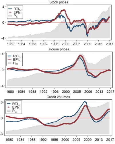
Figure 1 – Real-time and ex post financial imbalances

Note: These charts show the real-time and ex post financial imbalance measures for stock prices, house prices and credit volumes respectively, estimated based on equations 12 and 13. The sample period for estimating the cyclically adjusted fundamentals of these asset classes is January 1971 – June 2017, so the sample period for estimating these measures is January 1979 – June 2017. Each variable is normalised by its standard deviation. The real-time measures of financial imbalances are plotted in blue and the ex post measure in circled red. The shaded area plots the respective asset prices and credit volumes.

Despite different conditioning information, real-time imbalances 𝑅𝑅𝑅𝑅𝐼𝐼𝑗𝑗,𝑡𝑡 and ex post

measures 𝐸𝐸𝑃𝑃𝐼𝐼𝑗𝑗,𝑡𝑡share broadly similar patterns in each of the three financial markets (Figure 1).

The patterns are also consistent with the literature’s identification of financial boom and crisis episodes. For example, the stock market indicator identifies the boom in the late 1990s, as well

(16)

as the sharp contraction during 2000–2001, the dot-com bubble collapse.15 In the housing and

credit markets, the build-up in financial imbalances corresponds to the few years leading up to the GFC in 2008. Outside of these well-known episodes, the variations in the real-time and ex post financial imbalances are more moderate in size, but still not negligible.

2.3 Estimating the policy reaction function

This section turns to the estimation of the perceived US monetary policy reaction function. We start by first estimating the standard forward-looking Taylor rule over a rolling window, according to equation 9. The policy rate is the nominal fed funds rate up to 2009 when it reaches its effective lower bound, and a shadow rate afterwards (see Krippner (2013)). We use the Survey of Professional Forecasters’ median macroeconomic forecasts (SPF) as observables for expected inflation and unemployment. These variables are not subject to revisions, and capture policymakers’ apparent reactions as can be inferred in real time. The Taylor rule is estimated over

a rolling sample covering the average business cycle length of eight years.16 This approach is also

a simple way to approximate any non-linearities (such as asymmetric responses or threshold effects) in the policy rule, e.g. to allow for a ‘put’ strategy where the central bank reacts more to financial variables in busts than in booms.

We supplement this baseline analysis by estimating equation 9 with (i) the shadow rate of Wu and Xia (2016), (ii) nominal two-year interest rates as a proxy for the policy tool in the

period of unconventional policies following Hanson and Stein (2015)17, and (iii) Greenbook

forecasts over a smaller sample ending in 2012 (due to the five-year embargo). These alternative specifications are discussed in the robustness section 3.4.

On average, policy reacts positively to higher inflation and negatively to the unemployment rate in the usual way (Annex A2). But the estimated coefficients also exhibit significant time variations. Up to the GFC, the weight on inflation was relatively stable but then became less prominent as monetary policy entered crisis mode. The response to the unemployment rate generally remained countercyclical, except during the Volcker era when the weight on inflation increased as recessions were tolerated to bring inflation down. These time-varying estimates are consistent with previous studies such as Boivin (2006). More recently after the GFC, the response to the unemployment gap weakened, possibly as the FOMC’s lower bound on the policy interest rate constrained its ability to respond.

15 Phillips (2012) proposes a method of detecting a bubble-like behaviour, based on the unit-root property of the asset

price. We adapt this unit-root criterion in a robustness test and find that our approach yields similar inferences especially for episodes of wide swings in financial conditions.

16 For consistency, the windows for computing rolling regressions and moving averages are always eight years

throughout the paper. This window covers two terms of the Federal Reserve Chair (four years per term), and is close to the average time served by Fed Governors since the creation of the FOMC in 1935 (7.9 years). See FRB Kansas City (2009). Annex A2 shows the time-varying estimates of this standard Taylor rule specification.

17 An advantage of using an observable variable such as the two-year Treasury yield as the policy variable is that it avoids

(17)

To estimate the apparent policy sensitivity to financial variables, we regress the Taylor

rule residuals on our measures of financial imbalances, as well as control variables.18 We estimate

on a rolling sample basis:

𝜉𝜉𝑡𝑡=𝛽𝛽1,𝑡𝑡+𝛽𝛽𝑆𝑆,𝑡𝑡𝑅𝑅𝑅𝑅𝐼𝐼𝑆𝑆,𝑡𝑡+𝛽𝛽𝐻𝐻,𝑡𝑡𝑅𝑅𝑅𝑅𝐼𝐼𝐻𝐻,𝑡𝑡+𝛽𝛽𝐶𝐶,𝑡𝑡𝑅𝑅𝑅𝑅𝐼𝐼𝐶𝐶,𝑡𝑡+𝑧𝑧𝑡𝑡′𝛾𝛾𝑡𝑡+𝜀𝜀𝑡𝑡 (14)

where, 𝑧𝑧𝑡𝑡 is a vector consisting of annual changes in the oil price and the VIX index, the natural

candidates beyond inflation and output that investors think could be relevant for the central bank when setting policy. The loadings 𝛽𝛽𝑆𝑆,𝑡𝑡,𝛽𝛽𝐻𝐻,𝑡𝑡 and 𝛽𝛽𝐶𝐶,𝑡𝑡 track the systematic sensitivity of the monetary

policy instrument to the financial imbalance indicators. A positive (negative) loading represents a counter(pro)cyclical sensitivity to financial imbalances. These loadings are shown as the solid black lines in the left-column panels of Figure 2, and exhibit discernible variations over time.

Figure 2 – Estimated policy sensitivities to financial imbalances

Note: These charts show the sensitivity of the Taylor rule residuals to real-time measures of financial imbalances. Rows correspond to stock prices, house prices and credit volumes respectively. On the left column, dark lines represent estimates based on the baseline specification (equation 14). Green dotted lines are estimates based on a restricted specification where only one financial imbalance is included. Shaded areas represent 95% confidence intervals. The right column show policy sensitivities normalised by their time-varying standard errors. The sample period is January 1987 – June 2017.

We supplement these baseline loadings by three additional estimates. First, we restrict equation 14 to include only a single variable at a time (RTIS, RTIH or RTIC). This restriction imposes a strong assumption that each investor focuses narrowly on her market of specialty, ignoring the possibility that monetary policy could be reacting to many markets at the same time. While suffering from a potential omitted variable bias, this restricted specification evades any inference

18_{We have also controlled for some lags of the interest rate to take into account the persistence of the policy instrument,}

(18)

challenge associated with a high cross-market comovement.19 The resulting single-market

loadings are shown as green dashed lines on the left column of Figure 2.

The two remaining alternatives are the risk-adjusted counterparts of the previous ones, computed as the ratios of the point estimates and their standard errors. This adjustment takes into account the substantial time variations of estimates’ volatility (shaded areas on the left column), and allows investors to discount the loading estimates that are noisier. The risk-adjusted loadings, depicted on the right column of Figure 2, suggest that there were meaningful variations in policy reaction even in the second half of the sample. After adjusting for risks, policy loadings from the baseline and single-market models also appear more tightly correlated.

All four estimates suggest that US monetary policy has not systematically reacted to financial imbalances in a countercyclical way. This stands in contrast to the systematic and countercylical policy reaction vis-à-vis inflation and unemployment, the key mandate of the Federal Reserve. For the stock market, policy appears to be procyclical or neutral over a significant part of the sample. This includes almost the entire first half of the sample – only after the stock market bubble burst in early 2000s did policy reaction turn countercyclical. For the housing and credit markets, there is similarly no regular pattern of countercyclical policy reaction. In the mid-2000s before the crisis, all estimates notably suggest that monetary policy was either neutral or procyclical vis-à-vis imbalances in the housing and credit markets.

We exploit these variations in the policy loadings to examine their implications for subsequent financial imbalances. We choose the policy loadings from the multivariate model in equation 14 as the baseline to organise the results. However, we are agnostic about which policy loadings best represent investors’ perception, and replicate all key results with alternative loading estimates (see section 3.4). The main result of the paper holds in all cases.

2.4 Effects of policy reaction on the financial cycles

The final step is to assess whether estimated policy sensitivities to real-time financial imbalances can predict the developments of ex post financial imbalances. We estimate the local projection

specification using the ex post imbalance measure of each market 𝑗𝑗 as the dependent variable:

𝐸𝐸𝑃𝑃𝐼𝐼𝑗𝑗,𝑡𝑡+ℎ=𝛼𝛼ℎ+𝛼𝛼𝐵𝐵,ℎ𝐸𝐸𝑃𝑃𝐼𝐼𝑗𝑗,𝑡𝑡−1+𝛼𝛼𝑖𝑖,ℎ𝑖𝑖𝑡𝑡+𝛼𝛼𝜋𝜋,ℎ𝛽𝛽𝜋𝜋,𝑡𝑡+𝛼𝛼𝑈𝑈,ℎ𝛽𝛽𝑢𝑢,𝑡𝑡… +𝛼𝛼𝑆𝑆,ℎ𝛽𝛽𝑆𝑆,𝑡𝑡+𝛼𝛼𝐻𝐻,ℎ𝛽𝛽𝐻𝐻,𝑡𝑡+𝛼𝛼𝐶𝐶,ℎ𝛽𝛽𝐶𝐶,𝑡𝑡+𝜀𝜀ℎ,𝑡𝑡

(15)

where ℎ is the time lag between policy and ex post imbalance measures (up to 36 months). The

independent variables include lagged ex post imbalances, the nominal interest rate level, policy sensitivity to inflation and unemployment, and policy sensitivity to real-time imbalances in each

19 This tradeoff may be important in the late 1990s to early 2000s where housing and credit imbalances were most

correlated, and the gaps between the baseline and single-variable estimates largest. Even if ‘collinearity’ was a serious issue, investors may still want to use the multivariate model and do their best to disentangle monetary policy responses to different markets. Indeed, the FOMC minutes in the early 2000s suggest that the Fed recognised distinct drivers of the housing and credit developments, as well as their different implications. The FOMC linked elevated house prices to strong income, low long-term interest rates, and possibly speculation. By mid-2005, this led to an active debate regarding the role of monetary policy. Meanwhile, the FOMC viewed strong loan growth and mortgage refinancing activity over this period as generally positive for aggregate spending, as they indicated equity extraction.

(19)

financial market 𝑗𝑗.20 We compute heteroskedasticity and autocorrelation robust Newey-West

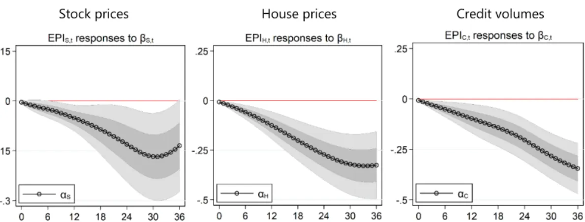
standard errors assuming that the autocorrelation dies out after three months. Figure 3 – Responses of financial imbalances to policy loadings

Stock prices House prices Credit volumes

Note: These charts show the dynamic responses over 36 months of the ex post imbalances for stock prices, house prices and credit volumes respectively (estimated with equation 15) to changes in thepolicy loadings on real-time imbalances for stock prices, house prices and credit volumes respectively (estimated with equation 14). Each variable is normalised by its standard deviation. The sample period is January 1987 – June 2017. Grey areas show 68% and 95% confidence intervals, computed with heteroskedasticity and autocorrelation robust standard errors.

Greater policy sensitivity to market 𝑗𝑗 has a consistently negative effect on the ex post

imbalances across the three markets and at all horizons considered (Figure 3). A monetary policy

reaction function that appears to lean against growing imbalances in real time tends to be

associated with a subsequent decline in the degree of imbalances in that particular market. The effect is also generally quite persistent, typically strongest after three years. The estimate is in the same order of magnitude for the three markets, slightly weaker in the equity market compared with the housing and credit markets. For example, a percentage point increase in the policy sensitivity to stock price developments reduces the subsequent imbalance in the market measure

by 0.15 standard deviation after 30 months.21

Could policy sensitivity to imbalances induce a dampening effect because this signals a higher interest rate path in the future, another guise of the narrow risk-taking channel? To disentangle the reaction function channel from this possibility, we augment equation 15 with survey measures of private expectations of future short-term interest rates (from the SPF). The results (shown in Annex A5) confirm the importance of the reaction function channel even after controlling for expected interest rate path.

20 Using an observable price/earnings ratio (PE) in place of an estimated measure of equity imbalances does not affect

the main result (Annex A3). Neither does allowing for a more general lag structure in equation 15 with up to three lags of the endogenous variable and the policy instrument (Annex A4).

21 The standard deviation of stock prices to their fundamentals is around 30% of the average value of stock prices over

the sample considered, so a decrease of 0.15 SD in the stock boom-bust measure represents a 4.5% decrease in the stock price deviation to earnings. A decrease of 0.3 SD in the housing boom-bust measure represents a 5.5% decrease in the house price deviation to rents. A decrease of 0.3 SD in the credit boom-bust measure represents a 3% decrease in the credit volume deviation to GDP.

(20)

Could the result be driven by policy responses to negative financial shocks – e.g. could a stock market crash induce both an immediate policy rate cut and lower stock prices subsequently? To examine this possibility, we augment equation 15 with the VIX index at horizons h = 0, 12, 24 and 36 months to control for the effect of financial shocks. As Annex A6 shows, the dampening effect of the reaction function channel survives this extension.

Any reverse causality bias – i.e. policy reacts more to financial imbalances because the central bank anticipates larger financial booms – should not be a major concern for two reasons. First, the central bank is less likely to respond to forecasts of imbalances further out in the future, making any reverse causality bias less severe the longer the horizon. Second, to the extent that the central bank intends to act countercyclically, the sign of the reverse causality bias would be positive, implying a stronger reaction function channel than the baseline estimates suggest.

(21)

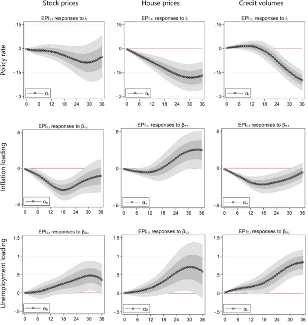
Figure 4 – Responses of imbalances to the policy rate and loadings on macroeconomic variables

Stock prices House prices Credit volumes

Po lic y r at e In flat io n lo adi ng Un em plo ym en t lo adi ng

Note: These charts show the dynamic responses over 36 months of the ex post financial imbalances for stock prices, house prices and credit volumes respectively to changes in the policy instrument and to changes in policy loadings on expected inflation and unemployment, estimated with equation 15. Each variable is normalised by its standard deviation. The sample period is January 1987 – June 2017. Grey areas show 68% and 95% confidence intervals, computed with heteroskedasticity and autocorrelation robust standard errors.

(22)

3. Extensions

3.1 Risk-taking channel and sensitivity to unemployment and inflation

The policy rate as well as policy loadings on macroeconomic variables also significantly influence the evolution of financial imbalances (Figure 4). A higher nominal interest rate deflates imbalances in all three markets, confirming the presence of a narrow risk-taking channel. Moreover, a greater sensitivity to inflation has a dampening effect on the stock and credit markets, with a more ambiguous impact on the housing market. Finally, a less sensitive response to labour market slack tends to encourage financial imbalances in all three markets. Strikingly, all these results are consistent with the findings of Bianchi et al (2018), i.e. low asset valuations tend to coincide with a higher interest rate, a greater responsiveness of policy rate to inflation, and a lower sensitivity of policy to output growth.

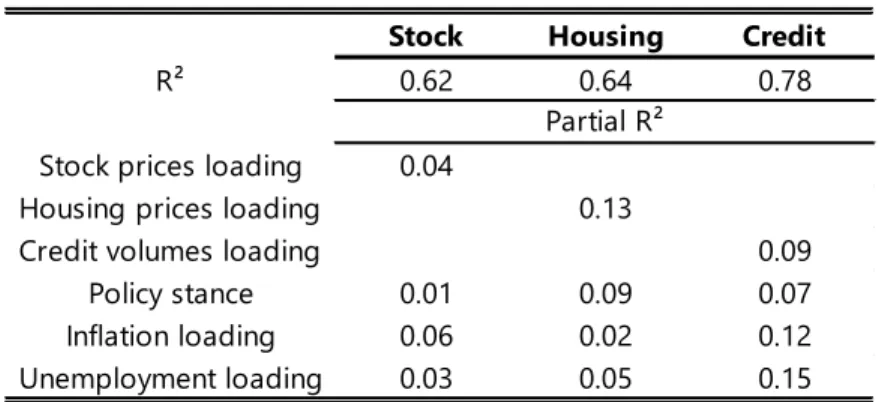
Table 1 – Variance decomposition

Note: This table shows the overall variance of the ex post financial imbalances explained by equation 15 for the three financial markets considered – the R² measure. It also shows the average variance, over 36 months, explained individually by the policy loadings on corresponding real-time financial imbalances, loading on the two macroeconomic variables, and the policy stance – the partial R² measure.

Quantitatively, the reaction function channel appears just as important as these other channels, if not more so. When estimating equation 15, we compute the partial R² of the policy loadings on financial imbalances, and do the same for policy loadings on macro variables and the level of policy rate for comparison. As Table 1 shows, the policy loadings on financial imbalances explain 4–13% of the variance of ex post imbalances over 36 months. The level of policy rate explains about 1–9%. Inflation and unemployment loadings explain 2–15% of the variance of ex post imbalances. For all three financial markets, the contribution of the reaction function channel is at least comparable to the alternative channels, and is highest in the case of the housing market.

3.2 The role of a central bank put

An asymmetric policy reaction vis-à-vis booms and busts could also influence financial risk-taking. In particular, a ‘central bank put’, i.e. a perception that policy will ease strongly in busts but remain inactive in booms, could provide greater incentives to speculate by limiting the tailed-event capital loss. A central bank put perception could thus further strengthen financial risk-taking in

Stock Housing Credit

R² 0.62 0.64 0.78

Stock prices loading 0.04

Housing prices loading 0.13

Credit volumes loading 0.09

Policy stance 0.01 0.09 0.07

Inflation loading 0.06 0.02 0.12

Unemployment loading 0.03 0.05 0.15

(23)

addition to our reaction function channel.22 Echoing the earlier findings of Borio and Lowe (2004),

we find some evidence of an ex post central bank put for the stock market, with lower financial imbalances being associated with greater policy sensitivity (Table 2, first three columns).

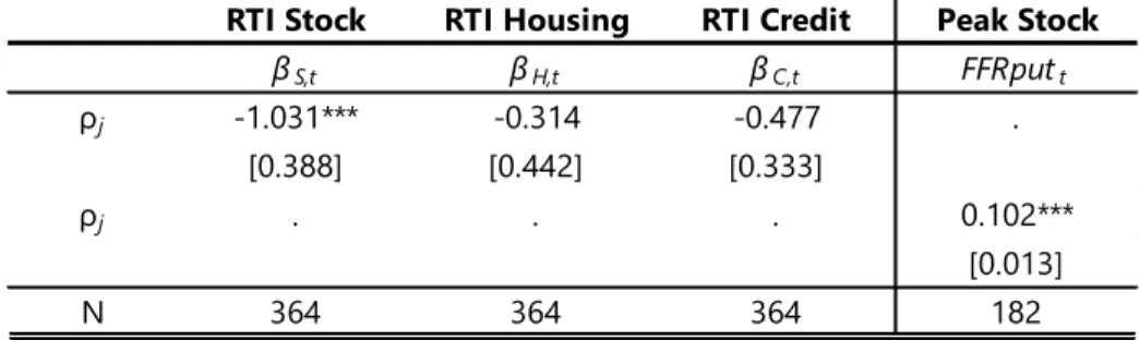
Table 2 – Correlation between policy sensitivity and financial imbalances and between a put perception and peaks of financial cycles

Note: The first three columns of this table show the correlation between policy sensitivity to a given financial variables and the real-time imbalance for that variable, by regressing the former on the latter. The last column shows the correlation between the variable FFRput and real-time stock price imbalances. FFRput is defined as 𝑝𝑝𝑝𝑝𝑐𝑐𝑝𝑝(𝐹𝐹𝐹𝐹𝑅𝑅 ≤ 𝐹𝐹𝐹𝐹𝑅𝑅𝑚𝑚𝑚𝑚𝑚𝑚𝑒𝑒−50𝑝𝑝𝑝𝑝)− 𝑝𝑝𝑝𝑝𝑐𝑐𝑝𝑝(𝐹𝐹𝐹𝐹𝑅𝑅 ≥

𝐹𝐹𝐹𝐹𝑅𝑅𝑚𝑚𝑚𝑚𝑚𝑚𝑒𝑒+ 50𝑝𝑝𝑝𝑝), where 𝐹𝐹𝐹𝐹𝑅𝑅 is the fed funds rate and 𝐹𝐹𝐹𝐹𝑅𝑅𝑚𝑚𝑚𝑚𝑚𝑚𝑒𝑒 is the mode of the market-implied

distribution of 𝐹𝐹𝐹𝐹𝑅𝑅, nine months ahead. This skewness measure serves as a proxy for central bank put. Peak Stock is a dummy variable that equals 1 during the 12 months leading up to peaks in stock price cycles.

For a policy put to affect risk-taking, it must be anticipated before a bust materialises. To measure the degree of put perception ex ante, we use a market-implied probability distribution of the future fed funds rate from the overnight index swap (OIS). We construct a skewness measure of this distribution, as the probability of the fed funds rate falling more than 50 basis points below the mode minus the conjugate probability that it will be more than 50 basis points above the mode, over a nine-month horizon (the longest available with reliable liquidity). A higher number indicates the policy rate distribution is tilted to the downside – a crude gauge of a policy put. This measure is positively associated with peaks of stock price cycles, so that the perception of a central bank put is higher during the later stage of a stock market boom (Table 2, last

column).23 The result is consistent with the interpretation that, even when investors foresee a

greater chance of a stock market crash, they simultaneously expect a Fed rescue in that event and hence continue to take on more risk than otherwise.

22 Like the reaction function channel, the effect of a central bank put operates through the anticipated response of

policymakers. We differentiate them because the mechanisms through which they affect risk-taking are different.

23 Because the binding zero lower bound period mechanically affects this skewness measure, we re-estimate this

coefficient outside of this period – the coefficient is smaller (0.069) but remains significant at the 1% level.

RTI Stock RTI Housing RTI Credit Peak Stock

βS,t βH,t βC,t FFRputt ρj -1.031*** -0.314 -0.477 . [0.388] [0.442] [0.333] ρj . . . 0.102*** [0.013] N 364 364 364 182

(24)

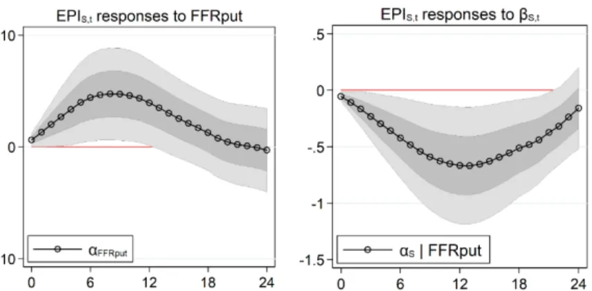
Figure 5 – Responses of stock market imbalances to put perception and policy loading on real-time stock imbalances

Note: The chart shows the dynamic responses over 36 months of the ex post stock price imbalances to changes in policy loadings on real-time stock imbalances, estimated with equation 15. Each variable is normalised by its standard deviation. The sample period is May 2002 – June 2017. Because of a smaller sample due to limited availability of market-implied probability, we estimate the dynamic responses over a shorter horizon, up to h=24 months. Grey areas show 68% and 95% confidence intervals, computed with heteroskedasticity and autocorrelation robust standard errors.

To jointly assess the impact of central bank put and the reaction function channel, we augment equation 15 with the perceived central bank put measure. Figure 5 plots the impulse responses of the stock market ex post imbalances to an increase in the central bank put perception (left) and the policy sensitivity to real-time imbalances (right). Findings suggest that the two channels coexist and operate alongside one another. A stock market boom can be propelled by both a weak policy reaction to it (the reaction function channel), and an anticipation that policy will ease strongly should the boom turns into a bust (the central bank put).

3.3 Boom-bust amplitudes

If the boom sows the seeds for the subsequent bust (Borio (2012)), then a policy reaction that mitigates the former could also reduce the severity of the latter. In this section, we investigate

whether a more countercyclical policy reaction reduces the amplitude of the boom-bust cycle, i.e.

containing not only the boom but also the extent of the bust once it occurs. This second-moment exercise complements the baseline case, which concerns the level effect of the policy reaction.

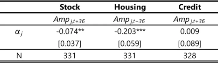
Our amplitude measure is the difference between the maximum and the minimum of the ex post imbalances over a rolling 36-month window. We estimate equation 15 using this amplitude measure as the dependent variable instead of the level of ex post imbalances. The results, shown in Table 3, suggest that a more countercyclical policy reaction significantly reduces the boom-bust cycle amplitudes in the stock and housing markets.

(25)

Table 3 – Boom-bust amplitudes

Note: This table shows the responses of the financial cycle amplitude,

𝐴𝐴𝐴𝐴𝑝𝑝𝑗𝑗,𝑡𝑡+36, to changes in thepolicy loadings on real-time imbalances for the

three financial markets. We define 𝐴𝐴𝐴𝐴𝑝𝑝𝑗𝑗,𝑡𝑡+36≡ 𝑠𝑠𝑢𝑢𝑝𝑝��𝐸𝐸𝑃𝑃𝐼𝐼𝑗𝑗,𝑡𝑡0− 𝐸𝐸𝑃𝑃𝐼𝐼𝑗𝑗,𝑡𝑡1� |𝑡𝑡0,𝑡𝑡1∈

[𝑡𝑡,𝑡𝑡+ 36]�, namely the difference between the maximum and the minimum of ex post imbalances over a 36-month period. Each variable is normalised by its standard deviation. The sample period is January 1987 – June 2017. ***, ** and * denote statistical significance at 0.01, 0.05 and 0.10 level respectively. Heteroskedasticity and autocorrelation robust standard errors in parentheses.

3.4 Robustness tests

The baseline findings are robust to various alternative measures of financial imbalances (real-time or ex post), estimates of policy loadings, and accounting for parameter uncertainty.

Alternative real-time imbalances

We consider three alternative real-time imbalances. First, we perform a log transformation of the level of the three financial variables to normalise their variation across time (Annex A7 plots the time series of log financial imbalances). The logarithm transformation linearises changes in time series such that the slope of the log data is approximatively equal to the percentage growth in the original series. With log data, percentage changes at any different points in time are comparable. Second, we re-estimate the regression of financial variables on their fundamentals (equation 12) using a fixed-size rolling sample rather than an expanding window. Third, we replace the current earnings in equation 12 by expectations of future earnings one year ahead to capture investors’ forward-looking expectations. Annex A7 depicts the resulting impulse responses, which confirm the main conclusions of the baseline model.

Alternative ex post imbalances

We consider three alternative ex post imbalance measures. The first is a log transformation of the baseline series (Annex A8 plots these variables). The second alternative is the product between the original measure 𝐸𝐸𝑃𝑃𝐼𝐼𝑗𝑗,𝑡𝑡 and its first and second differences:

𝑅𝑅𝐸𝐸𝑃𝑃𝐼𝐼𝑗𝑗,𝑡𝑡=𝐸𝐸𝑃𝑃𝐼𝐼𝑗𝑗,𝑡𝑡∗ Δ𝐸𝐸𝑃𝑃𝐼𝐼𝑗𝑗,𝑡𝑡∗ Δ2𝐸𝐸𝑃𝑃𝐼𝐼𝑗𝑗,𝑡𝑡 (16)

This triple-interaction object incorporates the higher momentum effects, recognising not only the size of financial imbalances but also when these gaps are growing and accelerating. This measure is closely related to the unit-root criterion of Phillips (2012) (see Annex A8 for the time series). As the third candidate, we borrow the bubble measure from Blot et al (2018) and use it as an externally identified boom-bust indicator. This method combines three different methodologies used in the literature – structural, econometric and statistical – to identify asset price bubbles in

Stock Housing Credit

Ampj,t+36 Ampj,t+36 Ampj,t+36

αj -0.074** -0.203*** 0.009

[0.037] [0.059] [0.089]

(26)

the stock and housing markets. The main result holds across these three alternative measures, as shown by the impulse responses reported in Annex A8.

Alternative policy reaction functions

We assess the robustness of our main result to four alternative Taylor rules. First, we use nominal two-year interest rates as the policy rate instead of a mix of the fed funds rate before 2009 and a shadow rate after. Second, we use the shadow rate of Wu and Xia (2016) in place of Krippner (2013). Third, we replace SPF inflation and unemployment forecasts by Greenbook forecasts. Fourth, we re-estimate the policy reaction function (equation 14) using real-time imbalances from only one financial market at a time to check for multicollinearity. As shown in Annex A9, none of these fundamentally changes the baseline results.

Accounting for parameter uncertainty

The estimated policy loadings entail parameter uncertainty, which we account for via two exercises. First, we construct risk-adjusted measures of the policy sensitivity, by normalising 𝛽𝛽𝑆𝑆,𝑡𝑡,𝛽𝛽𝐻𝐻,𝑡𝑡 and 𝛽𝛽𝐶𝐶,𝑡𝑡 by their respective standard error σj (see Figure 2 for time series). We do so for the baseline specification of equation 14 and for the alternative version that restricts equation 14 to include only a single financial variable at a time. These two measures allow for the possibility that investors adjust their risk-taking by less when they have a weaker conviction about the policy reaction function because it can only be estimated with a high degree of noise. As shown in Annex A9, these alternative measures of policy loading do not materially affect the baseline responses.

In the second exercise, we perform a Monte Carlo bootstrap-like estimation. We draw

2,000 complete time series for policy loading, taking an independent draw of 𝛽𝛽̂𝑗𝑗,𝑡𝑡 for each market

and each period at a time. In doing so, we assume 𝛽𝛽̂𝑗𝑗,𝑡𝑡 is normally distributed with means and

variances given by the first-stage baseline estimates.24 For each of the resulting 2,000 time series

of policy loadings, we then perform the second-stage estimation. Annex A9 shows the impulse responses from the exercise. A more countercyclical monetary policy now has a smaller dampening effect on financial imbalances in all three markets – the point estimates of impulse responses nearly halve. At the same time, the bootstrap standard error band is quite tight, and the estimated impulse responses remain highly significant in all cases. These results are therefore consistent qualitatively with the baseline finding.

Conclusion

Our study highlights the importance of the “policy reaction function” channel of monetary policy. We find that changes in the Federal Reserve’s apparent reaction function affect the development of US financial imbalances. When monetary policy appears less sensitive to financial conditions, financial imbalances tend to grow, potentially exacerbating the financial boom-bust cycles.

24 Because our empirical strategy relies on time variations of policy loadings, the standard block bootstrap is not feasible

(27)

Because we have controlled for monetary policy stance, both in terms of the current and the expected path of policy interest rate, this relationship is distinct from the standard risk-taking channel most studies focus on.

This result extends the vast empirical findings that risk-taking decisions depend on the levels of interest rates, and points at the more expansive effects of monetary policy through its systematic behaviour. Our investigation offers only an early glimpse into this rich and potentially rewarding avenue, and clearly further research is warranted. One empirical agenda is to use micro-level measures of perceived policy reaction function, e.g. based on surveys or internal reports at institutional levels, to examine if our findings can be corroborated. On the theoretical front, our findings call for incorporating the rich interactions between monetary policy-setting and market participants’ beliefs more fully into models used to guide policy.

In terms of policy implications, our findings provide new insights. To preserve financial stability, a central bank can do more than tighten policy on a discretionary basis when concerned about excessive risk-taking. Reacting systematically to developments of financial imbalances, and communicating such an intention even when financial stability risks may still be remote, can also yield benefits. Again, a useful analogy may be that of inflation stabilisation. The Taylor rule helps anchor inflation expectations because it provides economic agents with information about how policy would react to future shocks. In a similar vein, how market participants expect monetary policy to evolve with financial imbalances can endogenously determine the resulting financial boom-bust process. Our empirical finding has potentially far-reaching implications for the design of a macro-financial policy framework.

References

Adrian, T. and F. Duarte (2017): “Financial vulnerability and monetary policy”, Federal Reserve Bank of New York Staff Report, No. 804.

Adrian, T. and H. S. Shin (2010): “Financial intermediaries and monetary economics”, in Friedman,

B and M Woodford (eds.) Handbook of Monetary Economics, vol. 3, Elsevier.

Allen, F., G. Barlevy and D. Gale (2018): “A theoretical model of leaning against the wind”, Federal Reserve Bank of Chicago Working Paper, WP 2017-16.

Anufriev, M. and C. Hommes (2012): “Evolutionary Selection of Individual Expectations and

Aggregate Outcomes in Asset Pricing Experiments”, American Economic Journal: Microeconomics,

4(4): 35–64.

Bassetto, M., L. Benzoni and T. Serrao (2016): “The interplay between financial conditions and monetary policy shocks”, Federal Reserve Bank of Chicago Working Paper, 2016-11.

Bean, C. (2003): “Asset prices, financial imbalances and monetary policy: are inflation targets enough?”, BIS Working Papers, no 140, September.