Optimal Mortgage Design
Tomasz Piskorski
Stern NYU
[email protected]
Alexei Tchistyi
Stern NYU
[email protected]
November 20, 2006
AbstractThis paper studies optimal mortgage design. A borrower (a household) with limited liability needs …nancial support from a lender (a big …nancial institution) to purchase a home. We characterize the optimal allocation in a continuous time setting in which (i) the borrower’s income is volatile and its realization is unobservable to the lender, (ii) the lender has a right to costly foreclose the loan and seize the house, (iii) the borrower’s intertemporal consumption preferences are represented by a constant discount factor, (iv) the lender discounts cash ‡ows using a stochastic discount factor that depends on the market interest rate. We show that the optimal allocation can be implemented using either a combination of an interest only mortgage with a home equity line of credit or an option adjustable rate mortgage. Under the optimal contracts, mortgage payments and default rates are higher when the market interest rate is high. However, borrowers bene…t from low mortgage payments and low default rates when the market interest rate is low. Thus, our analysis provides theoretical evidence that these alternative mortgages, which have recently generated great controversy, can bene…t both lenders and borrowers.
We thank Andy Atkeson, V. V. Chari, Patrick Kehoe, Nobu Kiyotaki, Hanno Lustig, Christopher Phelan, Edward Prescott, Yuliy Sannikov, Martin Schneider, Ennio Stacchetti, James Vickery, and seminar participants at the Federal Reserve Bank of New York, Stern NYU, UCLA, and the Federal Reserve Bank of Minneapolis for helpful comments and suggestions. We are particularly grateful to Thomas Sargent and Stijn Van Nieuwerburgh for numerous discussions and suggestions.
1
Introduction
Recent years have seen a rapid growth in originations of more sophisticated alternative mortgage prod-ucts (AMPs), such as option adjustable rate mortgages (option ARMs) and interest only mortgages. In the United States, from 2003 through 2005, the originations of AMPs grew from less than 10% of residential mortgage originations to about 30%.1 As of the …rst half of 2006, 37%2 of mortgage originations were AMPs.
Option adjustable rate mortgages experienced particularly fast growth. They accounted for as little as 0.5% of all mortgages written in 2003, but their share soared to at least 12.3% through the …rst …ve months of 2006.3 As AMPs have complemented other forms of housing loans rather than replaced them, these
nontra-ditional mortgages account for a signi…cant part of the recent increase in household mortgage debt in the United States, from about 60% of GDP in 2003 to above 75% of GDP in 2006.4
Unlike traditional …xed rate mortgages (FRMs) and adjustable rate mortgages (ARMs), AMPs let bor-rowers pay only the interest portion of the debt or even less than that, while the loan balance can grow above the amount borrowed initially. Often, these mortgages carry teaser rates and come with a second mortgage, taking the form of a home equity line of credit (HELOC). Interest rates on such loans can increase as interest rates in the economy move higher. As a result of their popularity and the associated increase in the U.S. household debt, AMPs have generated great controversy and criticism. Critics contend that AMPs can hurt borrowers with high interest payments in the future.5 On the other hand, proponents say that AMPs allow
both lenders and borrowers to manage their cash ‡ows intelligently.
Surprisingly, despite of the economic signi…cance of AMPs and the extent of the surrounding controversy, there has so far been no attempt to formally address whether these new mortgages improve bene…ts to borrowers and lenders relative to traditional mortgages. In this paper, we formally address this question by formulating a general problem of …nding the best possible contract between a home buyer and a bank. Instead of considering a particular class of mortgages, we derive an optimal mortgage contract as a solution to a general dynamic contracting problem in a setting with as few assumptions as possible about payments between the borrower and the lender and about circumstances under which the home is repossessed. Then we examine whether features of existing mortgage contracts are consistent with the properties of the best possible contract.
Speci…cally, we consider a continuous-time setting in which a risk-neutral borrower with limited liability needs outside …nancial support from a risk-neutral lender in order to purchase a home. Home ownership generates for the borrower a public and deterministic utility stream. While the distribution of the borrower’s disposable income is publicly known, its realizations are privately observable by him. There is a liquidation
1United States Government Accountability O¢ ce (2006). 2Inside Mortgage Finance (2006a).
3Data from LoanPerformance, an industry tracker unit of First American Real Estate Solutions (FARES).
4The mortgage debt data are from Flow of Funds Accounts of the United States, Federal Reserve Board, and the GDP data
are from Bureau of Economic Analysis.
5See for example Department of the Treasury, Board of Governors of the Federal Reserve System, Federal Deposit Insurance
Corporation, National Credit Union Administration (2006), or United States Government Accountability O¢ ce (2006).
technology that allows termination of the relationship and transfer of the home to the lender. This transfer of ownership leads to ine¢ ciencies due to associated dead-weight costs. The focus on a risk neutral setup allows us to abstract from any possible insurance role of mortgages and to focus entirely on the fundamental feature of the borrowing-lending relationship with collateral, which is how to e¢ ciently provide a borrower with incentives to repay his debt using a costly liquidation.
An important assumption of our model is that the borrower and the lender have di¤erent discount rates. The borrower’s discount rate represents his intertemporal consumption preferences and is constant over time. On the other hand, the lender, a big …nancial institution, discounts cash ‡ows using a stochastic discount ratertthat depends on the market interest rate. To the best of our knowledge, this is the …rst paper
that allows for a stochastic interest rate in an optimal dynamic security design setting. We further assume that rt follows a two-state Markov process and is smaller than the borrower’s discount rate. We assume
that the borrower is more impatient than the lender re‡ecting that a borrowing-constrained household has a higher intertemporal marginal rate of substitution then a …nancial institution.
An allocation in this environment obligates the borrower to report his disposable income. The allocation speci…es transfers between the borrower and the lender, conditional on the history of the borrower’s reports and the circumstances under which the lender would foreclose the loan and seize the home. Although the borrower’s reports cannot be veri…ed, the threat of losing ownership of the home induces the borrower to pay his debt.
We characterize the optimal allocation using the borrower’s continuation payo¤atand the market interest
rate rt as state variables. Under the optimal allocation, the borrower truthfully reports his income. The
home is repossessed when the borrower’s continuation payo¤ at hits the borrower’s reservation utility A
for the …rst time. The borrower consumes part of his income whenever at reaches the upper boundary
a1(r
t). Whenat 2[A; a1(rt)], all the income of the borrower is transferred to the lender. The borrower’s
continuation payo¤ increases (decreases) when his income realization is high (low).
Interestingly, when the interest rate rt switches from high to low, the borrower’s continuation payo¤
jumps up. On the other hand, when the interest ratertswitches from low to high, the borrower’s
continu-ation payo¤ jumps down, which can trigger immediate bankruptcy. This is optimal because the stream of borrower’s payments is more valuable for the lender when the interest rate is low. As a result, the chances of home repossession are reduced by moving the borrower’s continuation payo¤ further away from the default boundaryAwhen the interest rate switches to low. However, the threat of repossession must be real enough in order for the borrower to share his income with the lender. As a result, the optimal allocation increases the chances of repossession when the interest rate is high in order to compensate for the weakened threat of repossession in the low state. This is done by moving the borrower’s continuation payo¤ closer to the default boundaryA when the interest rate switches to high.
After characterizing the optimal allocation in terms of the continuation payo¤s of the borrower and the lender, we examine whether features of existing mortgage contracts are consistent with the properties of
optimal allocation. We …nd that the optimal allocation can be implemented in three di¤erent ways using combinations of existing residential mortgage instruments. First, it can be implemented using an interest only mortgage with HELOC and two way balance adjustment. Second, it can be implemented using an interest only mortgage with HELOC with a preferential rate and one way balance adjustment. Third, it can be implemented using an option adjustable rate mortgage with a preferential interest rate. Therefore, our analysis provides theoretical evidence that the alternative mortgage products can be e¢ ciently utilized to mitigate agency cost in the stochastic interest rate environment.
Under the interest only mortgage with HELOC and two way balance adjustment, the borrower owns a home, while being obligated to make interest coupon payments on the interest only mortgage and interest payments on the home equity credit line balance. The parameters of HELOC are reset every time the market interest rate changes. When the market interest rate switches from high to low, the balance on HELOC is automatically reduced by an amount proportional to the outstanding balance and the interest rate charged on HELOC balance is also reduced. On the contrary, the balance and the HELOC interest rate are automatically increased when the market interest rate switches from low to high. The borrower uses his disposable income to make the current interest rate payments on the interest only mortgage and to repay the HELOC balance. When the disposable income realization is low, the borrower can draw on the credit line to make the current debt payments, as long as he does not exceed the credit limit. The borrower is in default if he is unable to make mortgage payments without exceeding the HELOC credit limit. In this case, the lender forecloses the loan and seizes ownership of the home.
Although mortgages with HELOC and two way balance adjustment are interesting from a theoretical point of view, we do not yet observe them in practice. While we actually observe reductions of mortgage debt balance in the form of "cramdown"6 provisions, the unusual feature of these mortgages is their automatic increase in debt balance in response to a market interest rate increase. The implementation using the interest only mortgage with HELOC with a preferential rate and one way balance adjustment addresses this issue.
The interest only mortgage with HELOC with a preferential rate and one way balance adjustment is similar to the interest only mortgage with HELOC and two way balance adjustment, except that a part of the HELOC balance is subject to a low preferential (teaser) rate and balance adjustment occurs only when the interest rate changes from high to low. This reduction in debt can be interpreted as an automatic "cramdown" provision to be applicable whenever the market interest rate switches to low. When the interest rate changes from low to high, the total amount of the HELOC debt does not change. Instead, the balance subject to the preferential rate shrinks.
The option ARM mortgage charges a low preferential interest rate on a portion of the balance. On the remaining part of the balance, a variable rate is charged which positively correlates with the market interest rate. The balance subject to the preferential rate increases when the interest rate switches from high to low
6"Cramdown" is a court-ordered reduction of the secured balance due on a home mortgage loan, granted to a homeowner
and decreases when the interest rate switches from low to high. Unlike the previous two implementations, here the interest rate changes do not a¤ect the total balance on the loan.
All three optimal mortgage implementations provide …nancial ‡exibility for the borrower to cover possible low income realizations. Given the interest only mortgage with HELOC and two way (or one way) balance adjustment, the borrower can draw on HELOC up to its limit, whenever his income is not su¢ cient to make the coupon payment. Under the option ARM, there is no minimum payment requirement – a low payment from the borrower translates into a higher balance, as long as the balance does not exceed the negative amortization limit. Although home repossession is costly, the borrower does not need to maintain precautionary savings, because the credit commitments by the lender provide a safety net.
The parametrized examples we consider indicate substantial e¢ ciency gains from using mortgage con-tracts that are contingent on the realization of the lender’s interest rate, such as the optimal option ARM or the interest only mortgage with HELOC, compared to contracts that do not depend on the lender’s interest rate. These examples also show that the e¢ ciency gains are largest for households that make little or no downpayment.
Critics of alternative mortgage products point out that AMPs seem to be more pro…table for lenders than traditional mortgages. They conclude that AMPs allow lenders to pro…teer at the expense of home-owners. However, this paper shows that the properties of AMPs are consistent with the properties of the optimal allocation governing the relationship between the borrower and the lender, which represents a Pareto improvement over traditional mortgages. As a consequence, it is possible that both lenders and borrowers bene…t from AMPs. Critics of AMPs have also raised concerns that teaser rates and low minimum payments can result in substantially higher mortgage payments and, as a consequence, higher default rates when in-terest rates in the economy increase. Nevertheless, this paper demonstrates that this possibility does not necessarily contradict optimality of AMPs. Under the optimal mortgage contract, mortgage payments and default rates are indeed higher when the market interest rate is high. However, borrowers bene…t from low mortgage payments and low default rates when the interest rate is low.
Related Literature
This paper belongs to the growing literature on dynamic optimal security design, which is a part of the literature on dynamic optimal contracting models using recursive techniques that began with Green (1987), Spear and Srivastava (1987), Abreu, Pearce and Stacchetti (1990), Phelan and Townsend (1991), among many others. Sannikov (2006a) developed continuous-time techniques for a principal-agent problem. The two studies that are most closely related to ours are DeMarzo and Fishman (2004) and its continuous-time formulation by DeMarzo and Sannikov (2006). These papers study long-term …nancial contracting in a setting with privately observed cash ‡ows, and show that the implementation of the optimal contract involves a credit line with a constant interest rate and credit limit, long-term debt, and equity. Biais et al. (2006)
study the optimal contract in a stationary version of DeMarzo and Fishman’s (2004) model and show that its continuous time limit exactly matches DeMarzo and Sannikov’s (2006) continuous-time characterization of the optimal contract. Tchistyi (2006) considers a setting with correlated cash ‡ows and shows that the optimal contract can be implemented using a credit line with performance pricing. Sannikov (2006b) shows that an adverse selection problem, due to the borrower’s private knowledge concerning quality of a project to be …nanced, implies that, in the implementation of the optimal contract, a credit line has a growing credit limit. Clementi and Hopenhayn (2006) and DeMarzo and Fishman (2006) o¤er theoretical analyses of optimal investment and security design in moral hazard environments.
Unlike this paper, none of the above studies considers an environment with a stochastic discount rate. We solve for the optimal allocation in the stochastic discount rate environment and …nd that its implementation involves a variable interest rate charged on the borrower’s debt as well as balance adjustments, adjustable preferential debt or a combination of both. On the technical side, building on the martingale techniques developed for Lévy processes, we extend DeMarzo and Sannikov (2006) characterization of the optimal allocation in a continuous-time setting to a stochastic discount rate environment.
There is a sizeable real estate …nance literature that addresses the design of mortgages in the presence of asymmetric information between the borrower and lender. The bulk of this literature focuses on adverse selection and how it a¤ects the menu of mortgages being o¤ered to borrowers with limited insurance possi-bilities. Chari and Jagannathan (1989) consider a model with two private types of borrowers, who di¤er in terms of the riskiness of their potential gains from selling the property, and show that the optimal contract to be chosen by borrowers with larger potential gains involves contractual arrangements such as points7 and
prepayment penalties together with a "due-on-sale" clause. Brueckner (1994) develops a model in which borrowers self-select into di¤erent loans, and shows that the optimal menu of mortgages will induce longer term borrowers to select loans with higher points and a lower coupon. Unlike these two papers, LeRoy (1996) considers a stochastic interest rate environment and …nds that, when borrowers re…nance optimally, if interest rates fall, the points/coupon choice can at best serve only to separate the least mobile borrower type from all others. Stanton and Wallace (1998) show that in the presence of transaction costs payable by borrowers on re…nancing, it is possible to construct a separating equilibrium in which borrowers with di¤ering mobility select …xed rate mortgages with di¤erent combinations of coupon rate and points. Posey and Yavas (2001) study how borrowers with di¤erent private levels of default risk would self-select between …xed rate mortgages and adjustable rate mortgages, and show the unique equilibrium may be a separating equilibrium in which the high-risk borrowers choose the adjustable rate mortgages, while low-risk borrowers select the …xed rate mortgages. Unlike these papers that focus on adverse selection, Dunn and Spatt (1985) consider a two-period moral hazard model, where future income realization of borrowers are uncertain and private, and show that the optimal mortgage would involve a due-on-sale clause. In terms of this literature, to our
knowledge, our paper is the …rst study of optimal mortgage design in a dynamic moral hazard environment, and the …rst study that addresses the optimality of alternative mortgage products.
There is also a large literature that focuses on the choice of mortgage contracts and the risk associated with them (for example, Campbell and Cocco (2003)). Unlike our paper, this literature takes a space of contracts as exogenously given, and studies the household choice within this restricted set of contracts. Another branch of research investigates limited participation models, where housing collateral insulates households from labor income shocks. Lustig and Van Nieuwerburgh (2005) typi…es this approach.
The paper is organized as follows. Section 2 presents the continuous-time setting of the model. Section 3 introduces the dynamic contracting model with a stochastic discount rate. Section 4 derives the optimal contract. Section 5 presents the implementations of the optimal contract. Section 6 discusses the approximate implementations of the optimal contract. Section 7 concludes.
2
Set-up
Time is continuous and in…nite. There is one borrower and one lender (or a group of lenders). The lender (a big …nancial institution) is risk neutral, has unlimited capital, and values a stochastic cumulative cash ‡ow fftg as E 2 4 1 Z 0 e Rtdf t 3 5;
where Rt is the market interest rate at which the lender discounts cash ‡ows that arrive at time t. We
assume that Rt= t Z 0 rsds;
whereris an instantaneous interest rate process, which takes values in the setfrL; rHg, where0< rL< rH:
We assume thatris a continuous-time process adapted toN, whereN=fNt;F1;t; 0 t <1gis a standard
compound Poisson process with the intensity (Nt)on a probability space( 1;F1; m1), such that fort 0 :
rt(Nt) = 8 < : r0 ifNtis even rc 0 ifNtis odd ; (Nt) = 8 < : (r0) ifNt is even (rc 0) ifNt is odd ;
wherer02 frL; rHgis given, andr0c=frL; rHg n fr0g:The above formulation implies that the interest rate
rate parameter (rt)of waiting times between successive changes. That is, for anyt 0;
P[rt+s=rL for alls2[t; t+ )jrt=rL] = e (rL) ;
P[rt+s=rHfor alls2[t; t+ )jrt=rH] = e (rH) :
The borrower (a household) is also risk neutral, has limited wealth, and values a stochastic cumulative consumption ‡owfCtgas E 2 4 1 Z 0 e tdCt 3 5:
We assume that, for all t; rt. The borrower can buy a home at date t= 0at price P:At any moment
in time, ownership of the home generates to the borrower a public and deterministic instantaneous utility equal to . The borrower’s initial wealth is Y0 0. We assume that P > Y0, so that the borrower must
obtain funds from the lender to …nance the purchase of a home.
A standard Brownian motionZ=fZt;F2;t; 0 t <1gon( 2;F2; m2)drives the borrower’s disposable
income process, where fF2;t; 0 t <1gis an augmented …ltration generated by the Brownian motion. The
borrower’s disposable income up to timet, denoted byYt, evolves according to
dYt= dt+ dZt; (1)
where is the drift of the borrower’s disposable income and is the sensitivity of the borrower’s income to its Brownian motion component. The borrower’s disposable income process,Y;is privately observed by him. In addition, the borrower maintains a private savings account. The private savings account balance,
S, grows at the interest rate t;which is adapted to the process r, and is such that for all t; t rt. The
borrower must maintain a non-negative balance at his account.
At any time, the relationship between the borrower and the lender can be terminated. In this case, the lender receivesL; while the borrower receives his reservation value equal toA. We assume thatA and that
rHL+ A < + ;
which ensures that the termination of the ongoing relationship is ine¢ cient.
Let( ;F; m) := ( 1 2;F1 F2; m1 m2)be the product space of( 1;F1; m1)and( 2;F2; m2):
3
Dynamic Moral Hazard Problem
At time0, the funds needed to purchase the home in the amount ofP Y0 are transferred from the lender
to the borrower. An allocation,( ; I);speci…es a termination time of the relationship, ;and the transfers between the lender and the borrower that are based on the borrower’s report of his income and the realized
interest rate process. Let Y^ = nY^t:t 0
o
be the borrower’s report of his income, where Y^ is (Y; r) -measurable. At any time0 t , the allocation transfers the reported amount,Y^t; from the borrower to
the lender, andIt( ^Y ; r)from the lender to the borrower. Below we formally de…ne an allocation.
De…nition 1 An allocation, = ( ; I);speci…es a termination time; ;and transfers from the lender to the
borrower,I=fIt: 0 t g;that are based on Y^ andr. Formally, is a( ^Y ; r)-measurable stopping time,
andI is a( ^Y ; r)-measurable continuous-time process, which is such that the process
E 2 4Z 0 e sdIsjFt 3 5
is square-integrable for0 t andY^ =Y:
The borrower can misreport his income. Consequently, under the allocation = ( ; I);up to time t , the borrower receives a total ‡ow of income equal to
(dYt dY^t)
| {z }
misreporting
+dIt;
and his private savings account balance,S, grows according to
dSt= tStdt+ (dYt dY^t) +dIt dCt; (2)
wheredCtis the borrower’s consumption at timet;which must be non-negative. We remember that, for all
t 0; St 0 and t rt:
In response to an allocation( ; I);the borrower chooses a feasible strategy that consists of his consumption choice and the report of his income in order to maximize his expected utility. Below we formally de…ne the feasible strategy of the borrower.
De…nition 2 Given an allocation = ( ; I);a feasible strategy for the borrower is a pair (C;Y^)such that
(i) Y^ is a continuous-time process adapted to(Y; r), and(Y Y^)process is of bounded variation, (ii) C is a nondecreasing continuous-time process adapted to(Y; r);
(iii) the savings process de…ned by (2) stays non-negative.
The borrower’s strategy is incentive compatible if it maximizes his lifetime expected utility in the class of all feasible strategies given an allocation = ( ; I). As a result, we have the following de…nition.
(i) given an allocation = ( ; I); the borrower’s strategy(C;Y^)is feasible,
(ii) given an allocation = ( ; I); the borrower’s strategy (C;Y^) provides him with the highest expected utility among all feasible strategies, that is
E 2 4Z 0 e t(dCt+ dt) +e AjF0 3 5 E0 2 4Z 0 e t(dCt0+ dt) +e AjF0 3 5
for all the borrower’s feasible strategies(C0;Y^0); given an allocation = ( ; I):
The above de…nition does not explicitly include the participation constraint imposing the condition that the borrower’s utility from the continuation of the allocation should be at least as large as the borrower’s outside option,A; which he can receive at any time by quitting. As the borrower can always under-report and steal at rate A until a termination time, any incentive compatible strategy would yield the borrower utility of at leastA.
The above de…nition of an incentive compatible strategy allows us to de…ne the incentive compatible allocation as follows.
De…nition 4 An incentive compatible allocation is an allocation = ( ; I), together with the
recommenda-tion to the borrower, (C;Y^); where(C;Y^)is a borrower’s incentive compatible strategy given an allocation
= ( ; I).
The allocation is optimal if it provides the borrower with his initial promised utilitya0and maximizes the
expected pro…t of the lender in the class of all allocations that are incentive-compatible. Below we provide a formal de…nition of the optimal allocation.
De…nition 5 Given the promised payo¤ to the borrower, a0, an allocation = ( ; I ), together with a
recommendation to the borrower (C ;Y^ ) is optimal if it maximizes the lender’s expected utility (expected pro…t): E 2 4Z 0 e Rt(dY^ t dIt) +e R LjF0 3 5
in the class of all incentive-compatible allocations that satisfy the following promise keeping constraint:
a0=E 2 4Z 0 e t(dCt+ tdt) +e AjF0 3 5:
In the following lemma, we show that searching for optimal allocations, we can restrict our attention to allocations in which truth telling and zero savings are incentive compatible.
Lemma 1 There exists an optimal allocation in which the borrower chooses to tell the truth and maintains
Proof In the Appendix.
The intuition for this result is straightforward. The …rst part of the result is due to the direct-revelation principle. The second part follows from the fact that it is weakly ine¢ cient for the borrower to save on his private account ( t rt) as any such allocation can be improved by having the lender save and make direct
transfers to the borrower. Therefore, we can look for an optimal allocation in which truth telling and zero savings are incentive compatible.
4
Derivation of the Optimal Allocation
In this subsection, we formulate recursively the dynamic moral hazard problem and determine the optimal allocation. First, we consider a problem in which the borrower is not allowed to save and we determine the optimal allocation8 in this environment. We know from Lemma 1 that it is su¢ cient to look for optimal
allocations in which the borrower reports truthfully and maintains zero savings, and so the optimal allocation of the problem with no private savings, for a given promise to the borrower, yields to the lender at least as much utility as the optimal allocation of the problem when the borrower is allowed to privately save. Finally, we show that the optimal allocation of the problem with no private savings is fully incentive compatible, even when the borrower can maintain undisclosed savings.
Methodologically, our approach is based on continuous-time techniques used by DeMarzo and Sannikov (2006). We extend their techniques to a setting with Lévy processes. Appendix A.2 derives the optimal allocation in a discrete-time version of our model.
4.1
The Optimal Allocation without Hidden Savings
Consider for a moment the dynamic moral hazard problem in which the borrower is not allowed to save. First, we will …nd a convenient state space for the recursive representation of this problem. For this purpose, we de…ne the borrower’s total expected utility received under the allocation = ( ; I) conditional on his information at timet, from transfers and termination utility, if he tells the truth:
Vt=E 2 4Z 0 e s[dIs+ ds] +e AjFt 3 5:
Lemma 2 The processV =fVt;Ft; 0 t < g is a square-integrableFt-martingale.
Proof follows directly from the de…nition of processV and the fact that this process is square-integrable,
which is implied by De…nition 1.
Below is a convenient representation of the borrower’s total expected utility received under the allocation
= ( ; I) conditional on his information at time t, from transfers and termination utility, if he tells the truth. LetM =fMt=Nt t (Nt);F1;t; 0 t <1gbe a compensated compound Poisson process.
Proposition 1 There existsFt-predictable processes ( ; ) =f( t; t); 0 t g such that
Vt = V0+ Z t 0 e s sdZs+ Z t 0 e s sdMs= V0+ Z t 0 e s s dYs ds | {z } dZs + Z t 0 e s s(dNs (Ns)ds): (3)
Proof We note that the couple(Z; N)is a Brownian-Poisson process, and it is an independent increment
process, which is a Lévy processes, on the space ( ;F; m):Then, Theorem III.4.34 in Jacod and Shiryaev (2003) gives us the above martingale representation for a square-integrable martingale adapted toFttaking
values in a …nite dimensional space (the process V).
According to the martingale representation (3), the total expected utility of the borrower under the allocation = ( ; I) and truth telling conditional on his information at time t equals its unconditional expectation plus two terms that represent the accumulated e¤ect on the total utility of, respectively, the income uncertainty revealed up to timet(Brownian motion part), and the interest rate uncertainty that has been revealed up to timet (compensated compound Poisson part).
According to Proposition 1, when the borrower reports truthfully, his total expected utility under the allocation = ( ; I)conditional on the termination time equals
V =V0+ Z 0 e s s dYs ds + Z 0 e s sdMs:
As Iand depend exclusively on the borrower’s report Y^ and the public interest rate process r, when the borrower reportsY ;^ by (3) he gets the expected utility, a0( ^Y), which equals
a0( ^Y) =E 2 6 6 6 4V0+ Z 0 e t t dY^t dt ! + Z 0 e t tdMt+ Z 0 e t(dYt dY^t) | {z }
payo¤ from stealing jF0 3 7 7 7 5= E V0+ Z 0 e t t dYt dt + Z 0 e t 1 t dYt dY^t + Z 0 e t tdMtjF0 : (4)
Note that because the process ( ; ) = f( t; t); 0 t g is Ft predictable; as for any t 0, s 0;
E0[Zt+s ZtjF0] =E0[Mt+s MtjF0] = 0;and given that E[V0jF0] =V0;we have that
a0( ^Y) =V0+E Z
0
Representation (5) leads us to the following formulation of incentive compatibility.
Proposition 2 If the borrower cannot save, truth telling is incentive compatible if and only if t
(m a:s:)for allt :
Proof Immediately follows from (5).
It is important to stress that in providing incentives for truth telling one can neglect an impact of reporting strategies on the magnitude of the adjustments, ; in the borrower’s promised value that occurs when the lender’s interest rate changes. It follows from (4) that, though in principle the reporting strategy of the borrower does a¤ect the magnitude of these adjustments, from the perspective of the borrower such adjustments have zero e¤ect on the borrower’s expected utility whatever is his reporting strategy. This property considerably simpli…es the formulation of incentive compatibility.
To characterize the optimal allocation recursively, we de…ne the borrower’s continuation value at timet
if he tells the truth as
at=E
Z
t
e (s t)[dIs+ ds] +e ( t)AjFt :
Note that for t we have that
Vt=
Z t
0
e s(dIs+ dt) +e tat:
But this, together with (3), implies the following law of motion of the borrower’s continuation value:
dat= atdt dt dIt+ tdZt+ tdMt= ( at t (rt))dt dIt+ tdZt+ tdNt: (6)
Here we discuss informally, using the dynamic programming approach, how to …nd out the most e¢ cient way to deliver a borrower any promised utilitya A. The proof of Proposition 3 formalizes our discussion below. Let b(a; r) be the highest expected utility of the lender that can be obtained from an incentive compatible allocation that provides the borrower with utility equal toagiven that the current interest rate is equal tor. To simplify our discussion we assume that the functionbis concave andC2in its …rst argument. Let b0 and b00 denote, respectively, the …rst and the second derivative of b with respect to the borrower’s
continuation utilitya.
We start by observing that transferring lump-sum dI from the lender to the borrower with promised utilitya;moves an allocation to that of the borrower’s promised utility ofa dI:The e¢ ciency implies that
which shows that for all(a; r)2[A;1) frL; rHgthe marginal cost of delivering the borrower his promised
utility can never exceed the cost of an immediate transfer in terms of the lender’s utility, that is
b0(a; r) 1:
De…ne a1(r); r 2 fr
L; rHg, as the lowest value of asuch thatb0(a; r) = 1: Then, it is optimal to pay the
borrower as follows
dI(a; r) = max(a a1(r);0):
These transfers, and the option to terminate, keep the borrower’s promised value betweenAanda1(r):But
this implies that whena2[A; a1(r)];and when the borrower is telling the truth, his promised value evolves
according to
dat(rt) = ( atdt dt dIt) + tdZt+ t(dNt (rt)dt): (8)
We need to characterize the optimal choice of process ( t; t); where t determines the sensitivity of the
borrower’s promised value with respect to his report, and t determines the adjustment of the borrower’s promised value due to a change in the interest rate. Using Ito’s lemma, we …nd that
db(at; rt) = ( at t (rt))b0(at; rt)dt +1 2 2 tb00(at; rt)dt+ tb0(at; rt)dZt+ [b(at+ t; rtc) b(at; rt)]dNt; whererc
t =frL; rHg n frtg. Using the above equation, we …nd that the lender’s expected cash ‡ows and the
change in the value he assigns to the allocation are given as follows:
E[dYt+db(at; rt)jFt] = + ( at t (rt))b0(at; rt) + 1 2 2 tb00(at; rt) + (rt) (b(at+ t; rct) b(at; rt)) dt:
From Proposition 2, we know that if t for all t then the borrower’s best response strategy is to report the truth, that is, Y^ = Y: Because at the optimum, at any time t; the lender should earn an instantaneous total return equal to the interest rate, rt, we have the following Bellman equation for the
value function rtb(at; rt) = max t , t A at 2 4 + ( at t (rt))b0(at; rt)+ 1 2 2 tb00(at; rt) + (rt) (b(at+ t; rct) b(at; rt)) 3 5: (9)
Given the concavity of the functionb(; rt),b00(at; rt) = d
2b(a
t;rt)
da2
t 0, setting
for allt is optimal. The concavity of the objective function in t in the RHS of the Bellman equation (9) also implies that the optimal choice of tis given as a solution to
b0(at; rt) =b0(at+ t; rtc); (10)
provided that t> A at;and otherwise t=A at. Note that this implies that t= (at; rt):
The lender’s value function therefore satis…es the following di¤erential equation
rtb(at; rt) = + ( at (at; rt) (rt))b0(at; rt)
+1
2
2b00(a
t; rt) + (rt) (b(at+ (at; rt); rct) b(at; rt)) (11)
withb(at; rt) =b(a1(rt); rt) (a a1(rt))forat> a1(rt)and the function speci…ed above.
We need some boundary conditions to pin down a solution to this equation and the boundaries a1(r);
r2 frL; rHg. The …rst boundary condition arises because the relationship must be terminated to hold the
borrower’s value to A, so b(A; rt) =L. The second boundary condition comes from the fact that the …rst
derivatives must agree at the boundary, sob0(a1(rt); rt) = 1:The …nal boundary condition is the condition
for the optimality ofa1(rt), which requires that the second derivatives match at the boundary. This condition
implies thatb00(a1(rt); rt) = 0, or equivalently, using equation (11), that
rtb(a1(rt); rt) = + a1(rt)
+ (rt) (a1(rt); rt) +b(a1(rt) + (a1(rt); rt); rct) b(a1(rt); rt) : (12)
By de…nition,a1(r)is the lowest value ofasuch thatb0(a; r) = 1;thus
(a1(rL); rL) = (a1(rH); rH) =a1(rH) a1(rL):
This, combined with (12) implies that
+ =rLb(a1(rL); rL) + a1(rL) (rL) b(a1(rH); rH) b(a1(rL); rL) +a1(rH) a1(rL) ;
+ =rHb(a1(rH); rH) + a1(rH) (rH) b(a1(rL); rL) b(a1(rH); rH) +a1(rL) a1(rH) :
The proposition below formalizes our …ndings.
Proposition 3 An optimal allocation that delivers to the borrower the value a0 takes the following form.
There exists boundaries: a1(r),r2 fr
(i) Ifa02[A; a1(r0)]; r02 frL; rHg; at evolves as
dat(rt) = ( atdt dt dIt) + (dY^t dt) + (at; rt)(dNt (rt)dt); (13)
and
–when at2[A; a1(rt)),dIt= 0;
–when at=a1(rt)the transfers dIt causeatto re‡ect at a1(rt):
(ii) Ifa0> a1(r0)an immediate transfera0 a1(r0)is made.
The relationship is terminated at time whenathitsA. The lender’s expected utility (expected pro…t) at
any point is given by a concave function b(at; rt), which satis…es:
rtb(at; rt) = + ( at (at; rt) (rt))b0(at; rt) + 1 2 2b00(a t; rt) + (rt) (b(at+ (at; rt); rct) b(at; rt)) (14)
when at is in the interval [A; a1(rt)] and b0(at; rt) = 1, when at > a1(rt), with boundary conditions
b(A; rt) =L and
+ = rLb(a1(rL); rL) + a1(rL) (rt) b(a1(rH); rH) b(a1(rL); rL) +a1(rH) a1(rL) ;
+ = rHb(a1(rH); rH) + a1(rH) (rt) b(a1(rL); rL) b(a1(rH); rH) +a1(rL) a1(rH) :
The function is de…ned as follows
(at; rt) = 8 > > > > > > < > > > > > > :
is a solution to b0(at; rt) =b0(at+ t; rtc)for all(at; rt)
for which the solution is such that (at; rt)> A at;
otherwise it is equal toA at
; (15)
whererc
t =frL; rHg n frtg:
Proof In the Appendix.
The evolution of the promised value (13) implied by the optimal allocation serves three objectives -promise keeping, incentives, and e¢ ciency. The …rst component of (13) accounts for -promise keeping. In order for at to correctly describe the lender’s promise to the borrower, it should grow at the borrower’s
discount rate, ; less the payment, dt, he receives from owning the home, and less the ‡ow of payments,
The second term of (13) provides the borrower with incentives to report truthfully his income to the lender. Because of ine¢ ciencies resulting from liquidation, reducing the risk in the borrower’s payo¤ lowers the probability that the borrower’s payo¤ reaches A, and thus lowers the probability of costly liquidation. Therefore, it is optimal to make the sensitivity of the borrower’s payo¤ with respect to its report as small as possible provided that it does not erode his incentives to tell the truth. The minimum volatility of the borrower’s promised value with respect to his report of income required for truth-telling equals 1. To understand this, note that, under this choice of volatility, underreporting income by one unit would provide the borrower with one additional unit of current utility through increased consumption, but would also reduce the borrower’s promised utility by one unit, so that this volatility provides the borrower with just enough incentives to report a true realization of income. Note that when the borrower reports truthfully, the term dY^t dt is driftless and equals to dZt.
The last term of (13) captures the e¤ects of changes in the lender’s interest rate process on the borrower’s promised utility. The optimal adjustments, , in the borrower’s promised utility, which are applicable when there is a change in the lender’s interest rate, are such that the sensitivity of the lender’s expected utility,b, with respect to the borrower’s promised utility,a, is equalized just before and after an adjustment is made.9
This sensitivity represents an instantaneous marginal cost of delivering the borrower his promised payo¤ in terms of the lender’s utility, and so the e¢ ciency calls for equalizing this cost across the states. We note that these adjustments imply the compensating trend in the borrower’s promised payo¤, (rt) (at; rt)dt,
which exactly o¤sets the expected e¤ect these adjustments have on the borrower’s expected utility.
Below we prove a useful lemma that characterizes the behavior of the optimal allocation when the borrower’s promised payo¤ is close to liquidation and there is an interest rate change.
Lemma 3 At the optimal allocation, there existsa2(A; a1(rL)]such that
- (A; rH) =a A;
- (a; rL) =A afora2[A; a]:
Proof From the de…nition of function b and the fact that rL < rH it follows that, for any a > A,
b(a; rL)> b(a; rH): This, together withb(A; rL) =b(A; rH) =L, implies that b0(A+; rL)> b0(A+; rH). Let
abe the smallesta > Asuch thatb0(a; rL) =b0(A+; rH). The existence of suchafollows from the fact that,
for any a2[A; a1(r
t)]; b0(a; rt) 1 andb0(a1(rt); rt) = 1: This combined with (15) yields us the alleged
properties of function .
Corollary 1 Lemma 3 implies that under the optimal allocation, whenever at 2 (A; a], an instantaneous
increase of the interest rate, rt;triggers the termination of the relationship.
4.2
The Optimal Allocation with Hidden Savings
So far we have characterized the optimal allocation under the assumption that the borrower cannot save. Now we show that, given the optimal allocation of the problem with no hidden savings, the borrower has no incentive to save at the solution, and thus the allocation of Proposition 3 is also optimal in the environment where the borrower can privately save.
Proposition 4 Suppose that the processatis bounded above and solves
dat= atdt dt dIt+ (dY^t dt) + tdMt (16)
until stopping time = minftjat=Ag;where tis anFt predictable process. Then the borrower’s expected
utility from any feasible strategy in response to an allocation ( ; I) is at most a0: Moreover, payo¤ a0 is
attained if the borrower reports truthfully and maintains zero savings.
Proof In the Appendix.
The above proposition shows that allocations from a broad class, including the optimal allocation of Proposition 3, remain incentive-compatible even if the borrower is allowed to privately save.
4.3
An Example
In this section we illustrate the features of the optimal allocation in a parametrized example. Table 1 shows the parameters of the model.
Table 1. Parameters of the model
Interest rate process Borrower’s discount rate Income process Utility ‡ow from home Liquidation values rL rH (rL) (rH) A L 1.5% 6.5% 0.2 0.2 8% 1 1 1 12.5 12
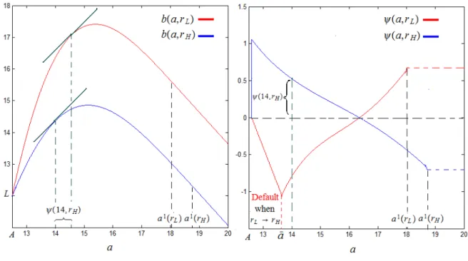
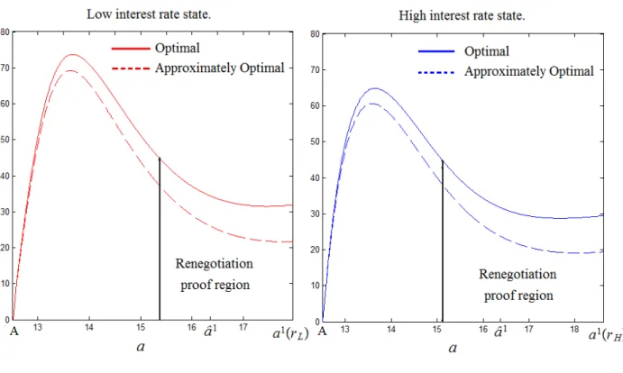
The left hand-side of Figure 1 shows the lender’s value function at both interest rates as a function of the borrower’s continuation value. For a given promise to the borrower, the value function of the lender at the low interest rate is always above the one at the high interest rate, except at termination when they are equal, as the lender attaches more value to the proceeds from the continuation of the relationship when his discount rate is lower. As we observe, it is optimal to allow the borrower to consume his disposable income earlier when the interest rate is low, that is a1(r
L)< a1(rH). Intuitively, when the lender’s interest rate is
Figure 1: The lender’s value function and the optimal adjustments in the borrower’s continuation utility.
future payo¤s and that of the lender is larger. To reduce this cost, it is optimal to allow the borrower to consume his excess disposable income earlier.
The right hand-side of Figure 1 shows the optimal adjustments in the borrower’s promised utility, , applicable when there is a change in the market interest rate. The borrower’s promised utility increases with a decrease in the interest rate and decreases with an interest rate increase, except in the area close to the re‡ection barriers when this relationship is reversed. The size of these adjustments is proportional to the distance of the borrower’s promise from the termination cuto¤ ofA.
The optimal adjustment of the borrower’s continuation utility, , is shaped by two competing forces stemming from, respectively, the costly termination of the relationship and the di¤erence in the discount rates. The closer the borrower’s continuation utility is to the termination boundary A; the bigger is the role played by the costly termination in shaping the optimal adjustment function. It is e¢ cient to reduce the chances of costly termination when the interest rate falls, as the stream of transfers from the borrower is more valuable for the lender when the interest rate is low. A reduction in the likelihood of termination is engineered by in‡uencing the borrower’s promise in two ways. First, it is optimal to instantaneously increase the borrower’s promise if the market interest rate falls, and this is even more so the more likely the relationship is to be terminated. Second, it is optimal to introduce a positive trend in the law of motion of the borrower’s continuation utility, which reinforces the …rst adjustment over time to the extent the interest rate stays low. As a result of these adjustments, the chances of costly home repossession are reduced by moving the borrower’s continuation payo¤ further away from the termination boundary A. However, the
threat of repossession must be real enough in order for the borrower to share his income with the lender. As a result, the optimal allocation increases the chances of repossession when the interest rate is high in order to compensate for the weakened threat of repossession in the low-interest state, both by instantaneously decreasing the borrower’s continuation utility and by introducing a negative trend in its law of motion.
If the borrower’s continuation utility is distant from the termination boundary A; then, intuitively, the discrepancy in the discount rates begins to play the dominant role in shaping the optimal adjustment function, as the likelihood of termination is small. When the lender’s interest rate switches to low, there is more tension between the borrower’s valuation of future payo¤s and that of the lender, and thus it is more costly to postpone the borrower’s consumption, the more so the bigger is his promise. To reduce this cost, it is optimal to decrease the borrower’s promise when the interest rate falls, by both an instantaneous adjustment and a negative time trend, provided that his prior promise was su¢ ciently large. In order to compensate for this reduction in the borrower’s promise when the interest rate switches to low, his continuation utility is increased to a range of high values of the borrower’s promise when the interest rate increases. It is important to observe that the adjustment of the borrower’s promise in this region has second order welfare e¤ects. This is because there is less di¤erence between the slopes of the lender’s value function at the low and at the high interest rate state, the further away the borrower’s promise is from the termination boundaryA:We will use this fact in Section 6, where we simply ignore the adjustments of the borrower’s promise in a region close to the re‡ection barriers.
5
Implementations of the Optimal Allocation
So far, we have characterized the optimal allocation in terms of the transfers between the borrower and the lender and the liquidation time of their relationship. In this section, we show that the optimal allocation can be implemented using …nancial arrangements that resemble the ones used in the residential mortgage market. We start with the following de…nition.
De…nition 6 The mortgage contract is optimal if it implements the optimal allocation of Proposition 3.
5.1
Interest Only Mortgage with Home Equity Line of Credit (HELOC) and
Two Way Balance Adjustment
In this section we consider a loan contract, which is a combination of two forms of debt - an interest only mortgage and a second "piggyback"10 mortgage that closes simultaneously with the …rst. Recently, there
has been a noticeable increase in the use of "piggyback" mortgages, and many lenders structure a second "piggyback" loan as a home equity line of credit. These lines are revolving lines of credit like credit cards, yet
1 0Named as such in the housing …nance industry because a second mortgage is "piggybacked" onto the original mortgage
they are secured by the borrower’s home collateral. Homeowners who pay o¤ the line of credit can continue to draw upon it and use the funds for other purposes. A de…nition below formally describes a contract that consists of an interest only mortgage with a home equity line of credit.
De…nition 7 Interest only mortgage with home equity line of credit and two way balance adjustment consists
of:
- Home equity line of credit with a time-t limit equal to CL
t: The initial balance equals B0: At any time
t, an instantaneous interest rate on the time-t balance, Bt; is equal to rt. If the balance on the credit
line exceeds its limit, default occurs.
- Balance adjustment, that is, an adjustment of the borrower’s balance on the home equity line of credit byBAt, applicable when there is an interest rate change.
- Interest only mortgage with a required coupon (interest payment) equal toxt:If the coupon is not paid
default occurs.
- When default happens, the lender receives the liquidation value of the home equal toL, and the borrower obtains the value of his outside option equal toA.
The proposition below shows that the optimal allocation can be implemented with a mortgage contract belonging to the class of contracts de…ned above.
Proposition 5 There exists an optimal interest only mortgage with HELOC and two way balance adjustment
that has the following features:
rt(Bt; rt) = + (rt) (a1(r t) Bt; rt) (a1(rt); rt) Bt ; (17) CtL(rt) =a1(rt) A; (18) xt(rt) = + a1(rt) + (rt) (a1(rt); rt); (19) BA(Bt; rt) = (a1(rt) Bt; rt) + (a1(rtc) a1(rt)): (20)
Under this mortgage contract, it is incentive compatible for the borrower to refrain from stealing. Once the borrower balance reaches zero, all excess disposable income is consumed by the borrower. With this mortgage contract, the borrower’s expected payo¤ , at, is determined by the current HELOC balance,Bt; as follows:
at=A+ CtL(rt) Bt =a1(rt) Bt: (21)
Proof In the Appendix.
How does the above implementation insure that the borrower refrains from stealing and consumes all excess disposable income only when his HELOC balance reaches zero? Given a time-t balance Bt on the
HELOC, the borrower can immediately consume all his available credit in the amount of CtL(rt) Bt and
default, which allows him to receive his outside option of A. But (21) implies that the payo¤ from this strategy is equal to at, which is the expected utility he would obtain by postponing consumption until his
HELOC balance is zero.
In the implementation of Proposition 5, the balance on the home equity line of credit can be considered as a memory device that summarizes all the relevant information regarding the past cash ‡ow realizations revealed by the borrower through repayments. The interest rate along with the required mortgage coupon payment, balance adjustment, and the credit line limit, determine the dynamics of the balance on the HELOC and the timing of default.
The adjustable features of the above mortgage contract are needed to implement the e¤ects of the changes in the interest rate on the borrower’s continuation utility. We remember that these adjustments take two forms - the instantaneous adjustment when the interest rate changes, and the compensating trend in the law of motion of the borrower’s utility. In the above implementation, the balance adjustment (20) implements the instantaneous adjustments in the borrower’s promised utility that are applicable when there is a change in the interest rate. The variable part of the interest rate (17) guarantees that a change in the borrower’s promised utility implied by the mortgage contract includes the trend that compensates the borrower, in expectation, for the instantaneous adjustments in his promise utility that happen when the interest rate changes.
The …xed component of the variable interest rate (17) on the HELOC insures that under the optimal strategy of the borrower, given the above mortgage contract, his promised utility increases at the rate of , as in the optimal allocation of Proposition 3. The mortgage coupon (19) guarantees that the change in the borrower’s promised utility implied by the mortgage contract re‡ects the reduction by the payments the borrower receives from owning the home. It also insures that an above-average income realization, and so an above-average repayment, increases the borrower’s promised utility, which corresponds here to a decrease in his HELOC balance, and vice versa. Finally, the dependence of the credit line limit (18) on the current interest rate mirrors the dependence of the re‡ection barriers,a1, on the interest rate in the optimal
allocation.
To further characterize the above mortgage contract we, will restrict our attention to the environment in which the optimal contract satis…es the following condition.11
Condition 1 The function implied by the optimal allocation is such that (a; rL)is strictly increasing in
afora2[a; a1(aL)];and so (a; rH)is strictly decreasing inafora2[A; a1(aH)], wherea is de…ned as in
Lemma 3.
Proposition 5, together with Lemma 3, implies the following properties of the above mortgage contract.
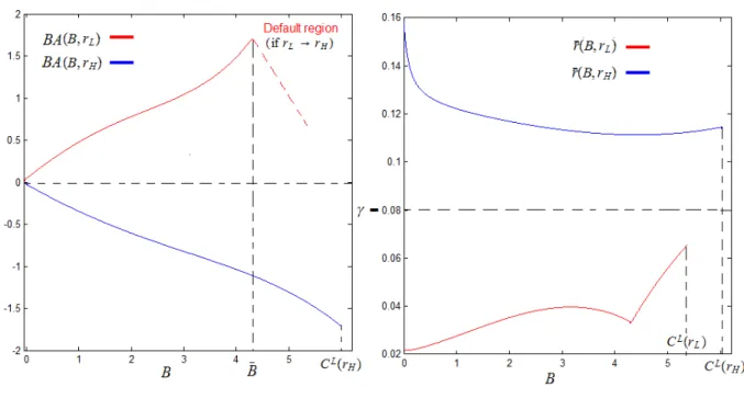
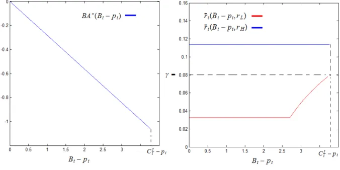
Figure 2: Optimal balance adjustment and the variable interest rate on the HELOC debt.
Corollary 2 The optimal interest only mortgage with HELOC and two way balance adjustment has the
following features: i) LetB=a1(r
L) awhereais de…ned in Lemma 3. Then, wheneverBt2[B; CtL(rL));an instantaneous
change of the interest rate fromrL torH triggers the default of the mortgage;
ii) BA(B; rt) = 0 for B = 0. Suppose further that the optimal function satis…es the properties of
Condition 1. Then,
–BA(B; rL)is positive and strictly increasing inB forB 2(0; B];
–BA(B; rH) is negative and strictly decreasing inB forB2(0; CtL(rH)];
–rt(B0; rL)< < rt(B00; rH); for anyB0 2[0; CtL(rL)]; B002[0; CtL(rH)]:
As the above corollary shows, under the optimal interest only mortgage with HELOC and two way balance adjustment, whenever the HELOC balance is close to the credit limit, an increase in the interest rate would cause the liquidation of the mortgage. Provided that the optimal adjustment function, , satis…es the properties of Condition 1, a decrease in the interest rate causes a decrease in the borrower’s HELOC balance and vice versa. The magnitude of these adjustments is proportional to the HELOC balance. The variable interest rate on the HELOC balance positively correlates with the lender’s interest rate. It is optimal to reduce mortgage payments, and as a result default rates, when the market interest rate is low because, in this case, the stream of borrower’s payments is more valuable for the lender. However, the threat
of repossession must be real enough in order for the borrower to share his income with the lender. As a result the optimal mortgage increases the chances of repossession when the interest rate is high in order to compensate for the weakened threat of repossession in the low state by requiring higher mortgage payments and default rates. Figure 2 presents the optimal balance adjustment and the variable interest rate on the HELOC debt in the parametrized environment of Section 4.3.
Although mortgages with HELOC and two way balance adjustment are interesting from the theoretical point of view, we do not yet observe anything like that in practice. While we actually observe reductions of mortgage debt balance in the form of "cramdown" provisions, the unusual feature of these mortgages is the automatic increase in debt balance in response to a market interest rate increase. Below we discuss an implementation using the interest only mortgage with HELOC with a preferential rate and one way balance adjustment that addresses this issue.
5.2
Interest Only Mortgage with HELOC with Preferential Rate and One Way
Balance Adjustment
In this section we consider a combination of an interest only mortgage with HELOC, where a part of the HELOC balance is subject to a preferential interest rate. The adjustment of the HELOC debt is only allowed when the lender’s interest rate declines. The de…nition below provides a formal description of this class of mortgage contracts.
De…nition 8 The interest only mortgage with HELOC with preferential rate and one way balance adjustment
consists of:
- HELOC with a time-t limit equal toCL
t(rt): The initial balance equals B0: At any time t, an
instan-taneous interest rate on a time-t balance, Bt; is equal to rpt on the portion of the balance below a
preferential range,pt 0, andrt on the portion of the balance above pt. If the amount of debt subject
to the preferential rate falls to zero, the mortgage is reset to other contract;
- Negative balance adjustment, that is the adjustment of the HELOC debt by BAt when the lender’s interest rate decreases;
- Interest only mortgage with a required coupon payment equal to xt: If the coupon is not paid, default
occurs;
- When default happens, the lender receives the liquidation value of the home equal toL, and the borrower obtains the value of his outside option, equal toA.
The proposition below shows that the optimal allocation can be implemented with a mortgage contract belonging to the class of contracts de…ned above.
Proposition 6 There exists an optimal interest only mortgage with HELOC with preferential rate and one way balance adjustment that has the following features:
rtp= 0; (22) rt(Bt pt; rt) = + (rt) (a1(rt) (Bt pt); rt) (a1(rt); rt) Bt pt ; (23) dpt= 8 < : (a1(rL) (Bt pt); rL) a1(rH) a1(rL) I(rt =rL) if Bt pt 0; if Bt< pt ; (24) BA (Bt pt) = (a1(rH) (Bt pt); rH) + a1(rL) a1(rH) ; (25) xt(rt) = + a1(rt) + (rt) (a1(rt); rt); (26) CtL(pt; rt) =pt+a1(rt) A: (27)
Under this mortgage contract, it is incentive compatible for the borrower to refrain from stealing. Once the borrower’s balance falls to the preferential debt limit, p, all excess disposable income is consumed by the borrower. For the debt balance Bt pt, the borrower’s expected payo¤ , at, is determined by the current
HELOC balance above the preferential debt limit, as follows:
at=A+ CtL(pt; rt) Bt =a1(rt) (Bt pt): (28)
If the amount of debt subject to the preferential rate falls to zero, the mortgage is reset to a contract that implements the continuation of the optimal allocation.
Proof In the Appendix.
The above implementation insures that the borrower refrains from stealing and consumes all excess disposable income only when his time-t HELOC balance, Bt, falls to the debt limit, pt, which is subject
to the preferential interest rate. Intuitively, given a time-t balance Bt on the HELOC, the borrower can
immediately consume all his available credit in the amount ofCL
t(pt; rt) Btand default, which allows him
to receive his outside option ofA. But (28) implies that the payo¤ from this strategy is equal toat, which is
the expected utility the borrower would obtain by postponing consumption until his HELOC balance falls to the preferential debt limit.
In the implementation of Proposition 6, the balance on the HELOC above the debt limit subject to the preferential interest rate can be considered as a memory device that summarizes all the relevant information regarding past cash ‡ow realizations revealed by the borrower through repayments. The interest rates, along with the required mortgage coupon payment, the negative balance adjustment, the preferential debt limit, and the credit line limit determine the dynamics of the balance on the HELOC and the timing of default.
As in the previous implementation, the adjustable features of the above mortgage contract are needed to implement the e¤ects of the changes in the interest rate on the borrower’s continuation utility. In the above implementation, the balance adjustment (25) implements the instantaneous adjustments in the borrower’s promised utility that are applicable when the lender’s interest rate decreases. The adjustments of the preferential debt limit (24) implement the instantaneous adjustments in the borrower’s promised utility that are applicable when the lender’s interest rate increases. The variable component of the interest rate (23) guarantees that a change in the borrower’s promised utility implied by the mortgage contract includes the trend that compensates the borrower, in expectation, for the instantaneous adjustments in his promise utility that happen when the interest rate changes.
The …xed component of the interest rate (23) on the HELOC balance above the preferential debt limit insures that, under the optimal strategy of the borrower, given the above mortgage contract, his promised utility would be increased at the rate of , as in the optimal allocation. The mortgage coupon (26) guarantees that a change in the borrower’s promised utility implied by the mortgage contract re‡ects the reduction by the payments the borrower receives from owning the home. The coupon also insures that an above average income realization, and so an above average repayment, increases the borrower’s promised utility, which corresponds here to a decrease in his HELOC balance, and vice versa. Finally, the dependence of the credit line limit (27) on the current interest rate mirrors the dependence of the re‡ection barriers,a1, on the current
interest rate in the optimal allocation.
In the proposed implementation, parameter p0 0 at time zero can be chosen arbitrary. One way to
initialize the mortgage is to set the market value of the mortgage equal to the book value:
B0=b r0; p0+a1(r0) B0 :
Proposition 6, together with Lemma 3, imply the following properties of the above mortgage contract.
Corollary 3 The optimal interest only mortgage with HELOC with preferential rate and one way balance
adjustment has the following features:
i) LetBt=pt+a1(rL) awhereais de…ned as in Lemma 3. Then, wheneverBt2[Bt; CtL(pt; rL));an
instantaneous increase in the lender’s interest rate triggers the default of the mortgage;
ii) BA (Bt pt) = 0forBt=pt. Suppose further that the optimal function optimal contract satis…es
the properties of Condition 1. Then,
–BA (Bt pt)is negative and strictly decreasing in (Bt pt)forBt2(pt; CtL(rH)];
–dpt 0 for any Bt pt; with strict inequality whenever the interest rate, rt, increases and
Bt> pt;
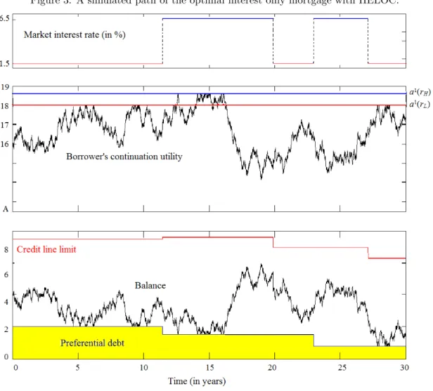
Figure 3: A simulated path of the optimal interest only mortgage with HELOC.
As the above corollary shows, under the optimal interest only mortgage with HELOC with preferential rate and one way balance adjustment, whenever the HELOC balance is close to the credit limit, an increase in the interest rate would cause the liquidation of the mortgage. If the optimal adjustment function, ;satis…es the properties of Condition 1, a decrease in the interest rate causes a decrease in the borrower’s HELOC balance. The magnitude of this adjustment is proportional to the HELOC balance. This adjustment can be interpreted as o¤ering the borrower an automatic "cramdown" provision, whenever the interest rate switches to low. An increase in the interest rate causes a drop in the amount of debt subject to the preferential interest rate. Consequently, under this contract, it is optimal to reduce the preferential treatment of the HELOC debt over time. We note that a declining preferential treatment of debt over time is a typical feature of many mortgage contracts currently o¤ered in the housing …nance market. As in the mortgage contract with variable interest rate and two way balance adjustment, the variable interest rate on the HELOC balance (23) positively correlates with the lender’s interest rate.
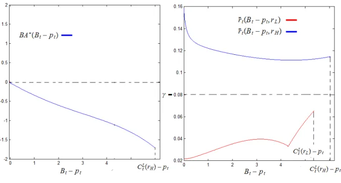
Figure 4: The optimal negative balance adjustment and the variable interest rate on the HELOC debt.
The top part of Figure 3 presents a simulated path of the market interest rate, the middle one presents a simulated path of the borrower’s continuation value under the optimal allocation, and the bottom one presents the behavior of credit line, the preferential debt range, and the HELOC balance implied by the optimal mortgage contract of Proposition 6, where the parameters of the model are set as in Section 4.3. Figure 4 presents the optimal negative balance adjustment and the variable interest rate on the HELOC debt in this parametrized example.
The implementation with an interest only mortgage and HELOC with one way balance adjustment avoids increasing the borrower’s debt when the interest rate changes from low to high by decreasing instead the amount of balance subject to the preferential rate. Similarly, one could avoid the reduction of the borrower’s debt (negative balance adjustment) when the interest rate decreases, by considering an implementation where the total amount of debt is left unchanged and instead, the balance subject to the preferential rate is increased. Below we discuss an implementation using the option ARM that exploits this idea.
5.3
Option Adjustable Rate Mortgage
In this section we consider an option ARM. This is an adjustable rate mortgage on which the borrower is o¤ered an option on how large a payment to make. A part of the mortgage debt is subject to the preferential interest rate. The de…nition below provides a formal description of this class of mortgage contracts.
- Mortgage debt with a time-t negative amortization limit equal to CtL: If the debt exceeds the negative amortization limit, default occurs. The initial balance is equal toB0 p0;
- At any timet, an instantaneous interest rate on a time-tdebt balance,Bt;is equal to a preferential rate
rtp on a part of the balance belowpt, andrt on a part of debt balance above pt. If the preferential
rate reaches its upper boundary , the mortgage is reset to other contract;
- When default happens, the lender receives the liquidation value of the home equal toL, and the borrower obtains the value of his outside option equal toA.
The proposition below shows that the optimal allocation can be implemented with a mortgage contract belonging to the class of contracts de…ned above.
Proposition 7 There exists an optimal option adjustable rate mortgage with preferential interest rate that
has the following features
rt(Bt pt; rt) = + (rt) (a1(r t) (Bt pt); rt) (a1(rt); rt) Bt pt ; if Bt pt (29) rpt(pt; rt) = + a1(r t) + (rt) (a1(rt); rt) pt (30) CtL(pt; rt) =pt+a1(rt) A (31) dpt= 8 < : (a1(r t) (Bt pt); rt) a1(rtc) a1(rt) dNt; if Bt pt 0; if Bt< pt : (32)
Under the terms of this mortgage, it is incentive compatible for the borrower to refrain from stealing and maintain balance Bt above pt. The borrower uses all available cash ‡ows to pay the balance whenBt> pt,
and consumes all excess cash ‡ows once the balance drops topt. For the debt balanceBt pt, the borrower’s
expected payo¤ ,at, is determined by the current balance above the preferential debt limit as follows:
at=A+ CtL(pt; rt) Bt =a1(rt) (Bt pt) (33)
If the preferential rate reaches its upper boundary , the mortgage is reset to a contract that implements the continuation of the optimal allocation.
Proof In the Appendix.
How does the above implementation insure that the borrower refrains from stealing and consumes all excess disposable income only when his time-t debt balance, Bt, falls to the debt limit, pt, subject to the
preferential interest rate given by (30)? Given a time-tbalanceBt, the borrower can immediately consume
all his available credit in the amount ofCL
t(pt; rt) Btand default, which allows him to receive his outside
the borrower would obtain by postponing consumption until his debt balance falls to the preferential debt limit.
As in the implementation with interest only mortgage and HELOC with preferential interest rate, the debt balance above the debt limit subject to the preferential interest rate can be considered as a memory device that summarizes all the relevant information regarding the past cash ‡ow realizations revealed by the borrower through repayments. The interest rates, along with the preferential debt limit, and the credit line limit, determine the dynamics of the debt balance and the timing of default.
As in the previous implementations, the adjustable features of the above mortgage contract are needed to implement the e¤ects of the changes in the interest rate on the borrower’s continuation utility. In the optimal option ARM, the adjustments of the debt subject to the preferential rate (32) implement all instantaneous adjustments in the borrower’s promised utility that are applicable when the lender’s interest rate changes. The variable component of the interest rate (23) guarantees that a change in the borrower’s promised utility implied by the mortgage contract includes the trend that compensates the borrower, in expectation, for the instantaneous adjustments in his promise utility that happen when the interest rate changes.
The …xed component of the interest rate (29) on the debt above the preferential debt limit insures that under the optimal strategy of the borrower, given the above mortgage contract, the borrower’s promised utility would be increased at the rate of as in the optimal allocation. The preferential interest rate insures that an above-average income realization and so an above-average repayment increases the borrower’s promised utility, which corresponds here to a decrease in his debt balance, and vice versa. Finally, the dependence of the credit line limit (31) on the current interest rate mirrors the dependence of the re‡ection barriers,a1, on the current interest rate in the optimal allocation.
In the proposed implementation, parameterp0 at time zero can be chosen arbitrarily, provided interest
raterp0 given by (30) is no greater than . One way to initiate the mortgage is to have the market value of the mortgage be equal to the book value:
B0=b r0; p0+a1(r0) B0 :
Proposition 7, together with Lemma 3, implies the following properties of the above mortgage contract.
Corollary 4 The optimal option ARM with preferential interest rate has the following features:
i) LetBt=pt+a1(rL) awhereais de…ned as in Lemma 3. Then, wheneverBt2[Bt; CtL(pt; rL));an
instantaneous increase in the lender’s interest rate triggers the default of the mortgage;
ii) Suppose further that the optimal function optimal contract satis…es the properties of Condition 1, then,