Automatic Labelling of Point Clouds Using Image Semantic Segmentation

UNIVERSITY OF TARTU

Institute of Computer Science

Computer Science Curriculum

Markus Loide

Automatic Labelling of Point Clouds

Using Image Semantic Segmentation

Master’s Thesis (30 ECTS)

Supervisor: Tambet Matiisen, MSc

Automatic Labelling of Point Clouds Using Image Semantic

Segmen-tation

Abstract:

Autonomous driving is often seen as the next big breakthrough in artificial intelligence. Autonomous vehicles use a variety of sensors to obtain knowledge from the world, for example cameras and LiDARs. LiDAR provides 3D data about the surrounding world in the form of a point cloud. New deep learning models have emerged that allow for learning directly on point clouds, but obtaining labelled data for training these models is difficult and expensive. We propose to use semantically segmented camera images to project labels from 2D to 3D, therefore enabling the use of cheaper ground truth data to train the aforementioned models. Furthermore, we evaluate the use of mature 2D semantic segmentation models to automatically label vast amounts of point cloud data. This approach is tested on the KITTI dataset, as it provides corresponding camera and LiDAR data for each scene. The DeepLabv3+ semantic segmentation model is used to label the camera images with pixel-level labels, which are then projected onto the 3D point cloud and finally a PointNet++ model is trained to do segmentation from point clouds only. Experiments show that projected 2D labels can be learned reasonably well by PointNet++. Evaluating the results with 3D ground truth provided with KITTI dataset produced promising results, with accuracy being high for detecting pedestrians, but mediocre for cars.

Keywords:

autonomous driving, deep learning, point cloud, semantic segmentation, projection

Automaatne punktipilvede märgendamine kasutades piltide

semanti-list segmentatsiooni

Lühikokkuvõte:

Isesõitvaid autosid loetakse tehisintellekti järgmiseks suureks saavutuseks. Need ka-sutavad mitmesuguseid sensoreid, nt kaamera ja LiDAR, et koguda infot ümbritseva maailma kohta. LiDAR salvestab andmed punktipilvena, milles iga punkt on esitatud kolmemõõtmeliste koordinaatidega. Uusimad sügavad närvivõrgud suudavad käsitleda punktipilve algsel kujul, kuid märgendatud andmete kogumine treeningprotsessi jaoks on keeruline ning kulukas. Käesoleva töö eesmärk on kasutada semantiliselt segmentee-ritud pilte 3D punktipilve märgendamiseks, võimaldades seeläbi koguda eelmainitud mudelite treenimiseks märgendatud andmeid odavamalt. Lisaks hindame olemasolevate semantilise segmenteerimise mudelite kasutamist suure koguse punktipilvede märgenda-miseks automaatselt. Meetodi testimärgenda-miseks kasutame KITTI andmestikku, sest see sisaldab nii kaamera kui ka LiDARi andmeid iga stseeni jaoks. Kaamera piltide pikseltasemel märgendamiseks kasutame DeepLabv3+ semantilise segmentatsiooni mudelit. Saadud märgendused projitseeritakse seejärel 3D punktipilvele, mille pealt treenitakse Point-Net++ mudel. Viimane on seejärel võimeline punktipilvi segmenteerima ilma lisainfota. Eksperimentide tulemused näitavad, et PointNet++ suudab projitseeritud märgendustest võrdlemisi hästi õppida. Tulemuste võrdlused objektide teadaolevate asukohtadega on paljulubavad, saavutades kõrge täpsuse jalakäijate tuvastamisel ning keskmise täpsuse autode tuvastamisel.

Võtmesõnad:

isesõitev auto, sügavad närvivõrgud, punktipilv, semantiline segmentatsioon, projektsioon

Contents

2.1.5 Pinhole camera model . . . 9

2.2 Object recognition . . . 11 2.3 Semantic segmentation . . . 12 2.4 Scene segmentation . . . 13 2.5 PointNet . . . 14 2.6 PointNet++ . . . 17 3 Methods 19 3.1 Pipeline . . . 19 3.2 Experiments . . . 22 3.3 Evaluation protocol . . . 23 4 Results 25 4.1 PointNet++ performance evaluation . . . 25

4.2 Ground truth evaluation . . . 30

4.3 Parameter tuning experiments . . . 34

5 Summary 36 Acknowledgements 37 References 40 Appendix 41 I. Licence . . . 41

1

Introduction

Autonomous driving is under active development, with more and more companies attempting to create semi- or fully autonomous cars [Cha17]. Many different sensors are used to acquire information from the surrounding world, such as cameras, radar, and ultrasonic [GLU12, Bar16]. Some companies are also using LiDAR, which provides information about the surrounding environment in the form of a 3D point cloud.

Recently deep learning models have been able to learn directly from point cloud data and perform object recognition on it. This benefit is limited by the fact that 3D ground truth data is difficult and expensive to obtain, as it requires working with 3D tooling and often also requires other data for context, such as camera images. Labelling images, however, is relatively easy and cheap. If the knowledge from labelled images could be transferred to unlabelled 3D data, acquiring new training data would become much cheaper.

If models for point cloud data can be trained more easily, they can be more useful as a standalone source of information about the surrounding world. This provides the ability to do predictions on point cloud data independently of other sensors. Having each sensor running its own models is beneficial for redundancy, as using a single model that requires input from all sensors means that if one sensor is defective for any reason, the entire pipeline stops producing meaningful predictions.

The goal of this work is to validate the approach of using 2D ground truth labels to train a model to predict 3D labels. To transfer 2D labels to 3D, we make use of geometrical transformations relying on the calibrations and transformations between camera and LiDAR. The challenges associated with this approach are:

• imperfect calibration resulting in geometrical alignment errors between camera and LiDAR,

• imperfect temporal alignment arising from different timings and acquisition delays in different sensors,

• imperfect labels due to errors in the labelling process,

The best performing methods on the KITTI benchmark [GLU12] using only point clouds [LVC+_{18, YML18, SWL18] rely on manually labelled data. Existing benchmark}

datasets and tasks have already gone through the trouble of annotating the 3D ground truth, so most research has been focused on training better models on these datasets, instead of obtaining training data and training models from less data. Using these models for a real-world system, however, has highlighted the problem of data gathering and labelling to a much bigger extent, so that it now becomes necessary to look for better solutions.

This work utilizes the KITTI object detection dataset that contains camera images and LiDAR point clouds to train a deep neural network model to perform scene segmentation (labelling each point with the appropriate class) on the point cloud data. For this end semantic segmentation using a pre-trained model was performed on the image data, after which the pixel labels were projected onto the point cloud data. The resulting labelled point cloud was then used to train a model that consumes point cloud coordinates and predicts the labels for each point. The results were then evaluated with regards how well the model learned to reproduce the noisy input, as well as how well the model is able to predict pedestrians, cars and cyclists compared to the ground truth.

This work is divided into the following parts:

• Chapter 2 presents the overview of the domain and introduces the theoretical background.

• Chapter 3 explains the experimental setup, describes the different experiments that were carried out and how they were evaluated.

• Chapter 4 details the results of the experiments.

• Lastly, the summary draws the final conclusions from the results and provides future directions for research.

The code for this work is publicly available1_.

2

Background

2.1

Sensors

2.1.1 Camera

Cameras are commonly used with autonomous vehicles for obstacle detection. This is mostly due to the availability of the sensor, as cameras are very widespread and as such, quite cheap. Moreover, cameras provide very high-resolution data compared to other sensors and also include color information [Bar16]. This large amount of data generated by the sensor allows for cameras to be used for deep learning when paired with appropriate labels, as for deep learning vast amounts of labelled data are key [noaa]. Despite the aforementioned, cameras also have downsides, the most notable of which are its inability to estimate depth well, its inability to deal with bad weather and dependency on ambient lighting [Bar16].

Dependency on good ambient lighting is one of the biggest downsides, because it renders the sensor much less useful at nighttime. Even with front-facing light illuminating the path, a lot less information will make it to the sensor. Additionally, weather conditions such as rain or snow can occlude objects in the camera’s field of view that might otherwise be visible [noa18].

Because a camera has no inherent way to detect depth, it must be estimated. This can, for example, be done using knowledge of the world, e.g. for humans their distance can be estimated from how prominent they appear on the image. This approach, however, might estimate a small child to be further away than they really are [Bar16].

There is another way to more reliably estimate depth that involves multiple cameras. An array of two cameras that are some distance apart is called a stereo camera and can be used to estimate depth using method called triangulation. Stereo cameras will be further discussed in section 2.1.3.

2.1.2 LiDAR

LiDAR (Light Detection And Ranging) is a sensing method that detects objects and maps their distances. The technology works by illuminating a target with pulsed laser light and measuring the characteristics of the reflected return signal. Distance is calculated using

the time-of-flight principle, that is, the sensor measures the time between emitting the laser pulse and the receiving the signal and calculates the distance. This makes LiDAR an active sensor - it provides its own source of energy, which also makes it independent of solar illumination [TI].

There are two main types of LiDAR systems: mechanical LiDAR and solid-state LiDAR. Mechanical LiDAR uses high-grade optics and a rotating assembly to achieve 360-degree field of view. This also results in a high signal-to-noise ratio over a wide field of view, but is at the same time bulkier. Solid-state LiDAR on the other hand has no rotating components and as such has a reduced field of vision, but is also cheaper because of this. Using multiple solid-state LiDARs in concert can mitigate the low field of vision with proper placement of sensors and combining their data.

2.1.3 Stereo camera

In addition to LIDAR, there are other sensors that can produce depth data, the most notable of which is the stereo camera. A stereo camera is a system of two cameras some distance apart [LSG08]. Depth data can be acquired by taking pictures simultaneously with both cameras, calculating the disparity map and projecting it to 3D space [GMM]. The disparity map encodes the difference in horizontal coordinates of corresponding image points [GMM], the depth is proportional to the inverse of disparity.

The main weaknesses of stereo cameras are similar to regular cameras: they do not operate well in low-light situations (evening, nighttime), whereas this is not a problem for LiDAR [Bar16]. Stereo cameras are also susceptible to rain and snow, albeit this is also a weakness of LiDAR [noaa]. For the stereo camera, additional computational work is needed to acquire depth information [GMM], which is not the case with LiDAR. When using a rotating LiDAR, the field of view covers 360 degrees around the vehicle, whereas achieving a similar field of view with stereo cameras requires multiple sensors placed accordingly [TI]. The maximum distance for stereo cameras is determined by how far apart the two cameras are, which limits it to around 40-50 meters for commercially available stereo cameras [noab, TI], whereas for LiDARs it is on the order of 100 meters [noac]. Due to the widespread use of cameras in general, the cost of stereo cameras is much lower than that of LiDARs.

2.1.4 Fusion

As both sensor types have their advantages and disadvantages, they could ideally be combined to benefit from the advantages of both [Bar16]. Combining this data is not trivial, as the camera sensor output is in the form of a 2D pixel array, whereas the LiDAR data is in the form of a 3D point cloud, each in their respective coordinate systems. Transforms between the coordinate systems can be done using affine transformations, which can be expressed as matrix multiplications. Equations for projection from 3D to 2D, however, can be derived using the assumption that the camera can be approximated by the pinhole camera model.

2.1.5 Pinhole camera model

The summary of the pinhole camera model has been adapted from the book by R. Hartley and A. Zisserman [HZ03] and an article by Yannick Morvan [Mor].

The pinhole camera model is the simplest mathematical model describing a 3D point’s projection onto a 2D image plane. While generally Euclidean geometry is used to describe objects in space, this has the drawback that points in infinity have to be modelled as a special case. The way around that is to instead use projective geometry, which allows for coordinates of points, even those at infinity, to be represented as finite coordinates. A three-element vector(X, Y, Z)T _{in Euclidean space would be represented}

as (X1, X2, X3, X4)T _{in projective space, whereX = X1/X4,Y = X2/X4,Z =}

X3/X4and X4 6= 0. These coordinates in projective space are called homogeneous coordinates.

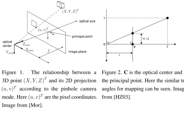
Let us consider the central projection of points in space onto a plane. Let the centre of projection - the optical center - be the origin of a Euclidean coordinate system and consider a plane atz =f from the origin called the (virtual) image plane. Heref is the focal length of the pinhole camera. The point where the optical axis intersects with the image plane is called the principal point. This is depicted on Figure 1.

Using this model, a point(X, Y, Z)T is mapped to the point on the image plane where a line joining this point to the centre of projection meets the image plane. Using the similar triangles method shown on Figure 2, it can be seen that this point is mapped to the point on the image plane with coordinates(f X_Z ,f Y_Z , f)T_{. Ignoring the final z-coordinate}

yields pixel coordinates(u, v)T _{= (}f X Z ,

f Y Z )

Figure 1. The relationship between a 3D point(X, Y, Z)T and its 2D projection

(u, v)T according to the pinhole camera mode. Here(u, v)T are the pixel coordinates. Image from [Mor].

Y Z f p C fY / Z

Figure 2. Cis the optical center andp

the principal point. Here the similar tri-angles for mapping can be seen. Image from [HZ03].

using homogeneous vectors, the previous can be written as

f X Z , f Y Z ,1 T →(f X, f Y, Z)T = (λu, λv, λ)T =λ(u, v,1)T. (1) Now the projection can instead be expressed as a simple linear mapping between the coordinates of these points as

λ    u v 1   =    f 0 0 0 0 f 0 0 0 0 1 0          X Y Z 1       , whereλ =Z. (2)

The previous expression assumes that the image plane point of origin is at the principal point of the image plane. In practice, the origin of the pixel coordinate system is commonly at the top left corner. With(σx, σy)

T

being the coordinates of the principal point, the previous expression can easily be modified to yield

λ    u v 1   =    f 0 σx 0 0 f σy 0 0 0 1 0          X Y Z 1       . (3)

This final equation is our perspective projection equation to map 3D points in the camera coordinate system to 2D points on the image plane.

To perform the perspective projection on points from another world coordinate system, the points must first be transformed into the camera coordinate system. This is done using an affine transformation that involves a rotation component and a translation component. Using homogeneous coordinates this perspective projection is

λ    u v 1   =    f 0 σx 0 f σy 0 0 1       r11 r12 r13 t1 r21 r22 r23 t2 r31 r32 r33 t3          X Y Z 1       , (4)

whererij are the rotational coefficients andti are the translational coefficients.

There are three main sources of errors when using these transformations and projec-tions - transformation errors, calibration errors and time-alignment errors. The first two are related to the pinhole camera model - if the sensors happen to move relative to each other’s positions during operation, the previously calculated transformation matrices are no longer correct, causing a bigger error the more the sensors have shifted. Calibration errors occur from improper camera calibration process and as such are constant. Time-alignment errors come about from differences in data acquisition frequency and start time. For example, a moving object might be captured by different sensors at slightly different time instances and because of it the 3D points of this object projected onto the image plane might not exactly fall onto the pixels depicting the same object.

2.2

Object recognition

Object recognition on images broadly falls to the following categories [LMB+14], as visualized on Figure 3:

• image classification - the image is given one or more labels based on the dominant objects depicted on it,

• object detection - bounding boxes are drawn around all detected objects on the image, which are also classified,

• semantic segmentation - each pixel of the image is labelled according to the class it belongs to,

• instance segmentation - each pixel of the image belonging to an object is labelled according to its class while differentiating between different instances of objects of the same class. The pixels belonging to the background are not labelled.

(a) Image classification (b) Object detection

(c) Semantic segmentation (d) Instance segmentation

Figure 3. Types of object recognition on images, images from [LMB+14].

2.3

Semantic segmentation

Semantic segmentation involves labelling each pixel of an input image according to some set of predefined classes. The input image does not have inherent limitations, it can be a monochrome image, an RGB image or have even more supplementary data attached to each pixel. The output is another image with the same pixel dimension as the input image, where each pixel is assigned a label. The label can be expressed as simple integer

or an RGB color with each label corresponding to a specific color. In the first case the output can be encoded as a grayscale image.

Common architectures to solve the semantic segmentation task are based on convolu-tional neural networks, such as fully convoluconvolu-tional networks [LSD15]. They downsample the original image to high-level features that are then upsampled for the final prediction in a single layer that uses feature maps from different layers. Other architectures, for example the U-Net [RFB15] are based on the previous fully convolutional networks, but instead of upsampling in a single layer at the end, the upsampling process is mirrored from the downsampling process and upsamples the feature map step by step. This architecture is also called an encoder-decoder architecture.

Another improvement to the encode-decoder architecture came from the DeepLab [CPK+_{18]. The encoder part of the network uses a ResNet-based [HZRS16] feature}

extractor network, which means that instead of simply learning a new feature map based on the previous feature map, it instead learns residuals or differences from previous maps. This helps alleviate vanishing gradients [HZRS16].

2.4

Scene segmentation

The semantic segmentation task extended to 3D point clouds is called scene segmentation or semantic scene understanding, an example of which is on Figure 4. In this task, each point of a 3D point cloud is assigned a corresponding class label. 3D point clouds can be assembled in various ways, for example the points can be acquired with LiDAR or a stereo camera. In addition to the point coordinates, LiDAR also records the surface reflectivity, whereas the stereo camera can also store the RGB data from either camera. While semantic segmentation is a well established task with state of the art architec-tures mostly based on encoder-decoder deep convolutional neural networks, this is not the case for scene segmentation. As point cloud data is not as structured as image data, there are more architectures available. According to Simon et al [SMAG19] there exist three main approaches to extend object recognition methods using deep learning to point cloud data:

• process the points into a voxel grid with voxels of a predetermined size and use 3D convolutional neural networks,

• use a multi-layer perceptron based network (i.e. not a convolutional or recurrent neural network) directly on the points,

• a combination of both.

Figure 4. An example of scene segmentation from the ScanNet dataset [DCS+17]. The image depicts predictions made on RGB-D data on the left and the ground truth on the right. While the raw input data is in point cloud format, the predictions and ground truth have been divided into a voxel grid.

2.5

PointNet

In the following we summarise the PointNet architecture from the paper [CQCS+17]. While the voxel grid is a straightforward method of preprocessing the point cloud into a structured format, the result contains a high number of voxels. In addition to the high volume, this process of quantizing points into voxels can also create artifacts, for example a voxel where the corners of two different objects meet is labelled as being one of the two classes, which means any knowledge of the other object in that voxel is effectively lost. Point clouds are simpler structures than grids, therefore learning from them should ideally also be simpler.

Point sets have a number of properties that need to be taken into account in the network design:

• They are unordered. A network that consumes point sets needs to be invariant to all possible permutations of data input.

• Interaction between points. Neighbouring points form a meaningful subset in the point set. The network needs to be able to capture local structure, as well as interactions between these local structures.

• Invariance under transformations. As the point set consists of points in Euclidean space, the labeling of the point set should be invariant to affine transformations.

There are three ways to approach processing unordered point sets for deep learning:

• sort the input before using it as an input to a network,

• treat input as a sequence and train a recurrent neural network (and augment the input using various permutations),

• use a symmetric function (where the output of the function is invariant to input order) to aggregate data from points.

Sorting appears to not work for this task, because slight perturbations of points can change the ordering too much. Using recurrent neural networks can work if the length of input is short (dozens of points), but this approach does not scale to an input of thousands, which is common for point cloud data. The last option - transforming elements in the point set and then applying a symmetric function has been shown empirically to work the best, despite its simplicity. Some examples of such symmetric functions are sum, average and max.

The PointNet architecture takes raw point clouds as input, represented by 3 coordi-nates. Other data, such as computed normals or handcrafted features can also be added as additional dimensions. In the case of classification, the network outputs class label scores for the entire input, whereas in the case of scene segmentation or part segmentation, the point label for each input point is produced instead.

The overall architecture of the network is simple - initially each point is processed independently and identically, after which a symmetric function in the form of max

pooling is applied. This causes the network to effectively learn a set of optimization functions or criteria that select interesting points carrying the most information, as well as encoding the reason for their selection. The final fully connected layers aggregate the previous information into a global signature, which can easily be classified. As segmentation also requires local knowledge, the input to the segmentation subnetwork is a concatenation of the global features and the per point features that act as new features that contain both local and global information. For the point set to be invariant under affine transformations, the network learns a special affine transformation in the form of a spatial transformer network called T-net. This network resembles the main network in architecture and is also learned once for the feature space. A visual representation of the architecture is depicted on Figure 5.

Figure 5. The input to the network are n points to which input and feature transformations are applied, after which point features are aggregated by max pooling, which is the symmetric function in this architecture. The output is k classification scores. The segmentation network is an extension of the classification network, which concatenates local and global features and outputs per point scores. “mlp” stands for multi-layer perceptron with the layer sizes in brackets. Image from [CQCS+17].

2.6

PointNet++

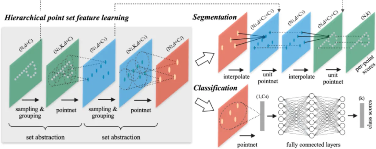
In the following we summarise the PointNet++ architecture from Qi et al [QYSG17]. The original PointNet’s main limitation is that it does not capture local structure very well, as it generates global features directly from pointwise features. Exploiting local structure, however, is one of the main reasons why convolutional architectures work so well. PointNet++ improves upon the original PointNet by processing point sets in a hierarchical manner, much like convolutional architectures. This approach combines the benefits introduced by convolutional architectures with the efficiency of not having to preprocess point sets into a more voluminous voxel grid.

To mimic a convolutional architecture, the points must first be partitioned into somewhat overlapping local regions, which allows for capturing fine structure from neighboring points. Features from these local regions are then grouped into larger units and processed to acquire higher level features using a local feature learner, for which the weights can be shared, similarly to convolutional networks.

For partitioning, a simple neighbourhood ball is used with farthest point sampling being used to cover all points. For the local feature learner, a PointNet is used, as it already solves the problem of learning feature vectors from point sets. This effectively means that PointNet++ applies PointNet recursively on the input point set.

These three operations define a set abstraction that is similar to a convolutional layer -Sampling, Grouping, PointNet. These set abstractions are then used to group the features from local regions into larger units and the process is repeated until features for the whole point set are obtained. This process is visualized on Figure 6.

Additionally, in real world point clouds point density varies in different areas, which means that some parts of the point cloud might be very sparse. The features learned on dense regions might not generalize to sparse regions and vice versa. While capturing details from the lowest possible level should be ideal for densely populated regions, it does not work for sparsely populated regions, where local patterns might be corrupted from the lack of points. In this case, larger-scale patterns should instead be inspected.

To solve this, the PointNet operation is changed to combine features from regions of different scales that is dependent on the input sampling density. This can be done in two ways - multi-scale grouping and multi-resolution grouping, visualized on Figure 7. Multi-scale grouping is a simple, yet effective way to capture multiscale patterns by

Figure 6. Illustration of the hierarchical feature learning architecture of PointNet++. In the visual examples, points from 2D Euclidean space are used. Image from [QYSG17].

applying grouping layers and PointNet layers at different scales concurrently and then concatenating the results of both. Multi-resolution grouping, however, takes the summary vector from the previous level of abstraction and concatenates it with the features obtained from processing the points directly. The latter approach is computationally more efficient, because the concatenated features are only computed once.

Figure 7. Multi-scale grouping (left) and resolution grouping (right). With multi-scale grouping different multi-scales of neighbourhoods are used to get features, whereas with multi-resolution grouping lower-level features are simply concatenated with the current-level features. Image from [QYSG17].

3

Methods

3.1

Pipeline

To evaluate learning 3D labels from 2D labelled data we have used the KITTI dataset [GLSU13]. This dataset was chosen because it contains both image and point cloud data, as well as all the necessary calibration and transformation data between different sensors. In addition the dataset and various prediction tasks are quite mature and the existing leaderboards provide for a good comparison2_{. An alternative to KITTI is the nuScenes}

dataset, which also provides image, LiDAR and radar data [CBL+19]. This dataset was not used in this work because it was not available at the start of experimentation.

Figure 8. An example of a camera image (top) and point cloud (bottom) from the KITTI dataset [GLSU13].

Image Semantic segmentation (DeepLabv3+) Projection Segmented image LiDAR point cloud

Labelled point cloud

PointNet++

Figure 9. The training pipeline that produces a trained PointNet++ model by generating semantic segmentation labels and projecting them onto point cloud data.

LiDAR point cloud PointNet++ Labelled point cloud

Figure 10. The prediction pipeline using a trained PointNet++ model to produce labels for point cloud input.

While the KITTI dataset has a semantic segmentation benchmark task with image and ground truth segmentation pairs, it only consists of 200 images that do not come with already matched point cloud scenes. Another available benchmark task, the 3D object detection task, comes with matched image, point cloud and 3D bounding box ground truth data. An example of the image and LiDAR data is on Figure 8. While the data in this task does not come with semantic segmentation ground truth, it provides around 7500 samples, matched image and point cloud data, as well as transformation and calibration matrices. To acquire necessary semantic segmentation labels for the images in this dataset, a pre-trained semantic segmentation network was used.

To obtain the semantic segmentation data for the images in the KITTI dataset, DeepLabv3+ [CZP+18] with the Xception backbone [Cho17], pre-trained on the CityScapes dataset [COR+16] was used. This pre-trained model was chosen because Xception per-formed the best out of the alternatives, which is preferable over speedier inference and the CityScapes dataset was the closest match to the KITTI dataset.

Using labelled images, the next step is to propagate these labels to the point cloud. The point cloud from LiDAR data is projected onto the image plane using the provided transformation and projection matrices with the end result being rounded to match

projected points to pixels properly. Any point projected outside the boundaries of the labelled image is discarded. Any remaining point now has a corresponding image pixel, the label of which is now used to also label the original point in the point cloud. It should be noted that this projection is not perfect, due to alignment problems some points might be labelled with neighboring classes. As neural networks are known to be quite robust to the labelling noise, our hope was that if the labelling noise is uniform, the network will learn to produce correct predictions regardless.

Not all CityScapes class labels are used, but a limited subset. The classes that were kept were chosen based on a number of considerations. Initially, if multiple classes corresponded to the same label color, only one of them was kept. After this, classes that had little semantic meaning (e.g. they did not correspond to an object in the real world, but were helper classes, such as the class “ego vehicle” that marks the vehicle carrying the sensors) or ones that were not present in the dataset were also omitted. In addition, the “unlabelled” class was kept for convenience of evaluation. The included classes are thus the following: unlabelled, road, sidewalk, building, wall, fence, polegroup, traffic light, traffic sign, vegetation, terrain, sky, person, rider, car, truck, bus, train, motorcycle, bicycle.

The resulting labelled point cloud is then saved for further processing. This in-cludes dividing the point cloud data into a training, validation, and test set, as well as transforming these to a format suitable for PointNet++.

To perform experiments using the PointNet++ architecture, the original implemen-tation written in TensorFlow is used with multi-resolution grouping method and with the max pooling symmetric function. The training set is used for training PointNet++ models and validation set is used to perform a simple hyperparameter search on domain-and architecture-specific parameters. From these experiments, the model that performs the best on the validation set is chosen for further evaluation on two test sets, with one using generated labels and the other using labels from 3D ground truth. The full training pipeline is depicted on Figure 9 and the prediction pipeline is on Figure 10.

3.2

Experiments

The original PointNet++ implementation uses a subsampling strategy for scenes, sam-pling a voxel with the size of 1.5 meters by 1.5 meters by 3.0 meters by randomly choosing a point from the scene to act as the center around which the voxel is constructed. The default value for voxel size is chosen by the authors according to the size of a human, i.e. so all of a human’s points could ideally fit into a sampled voxel. This voxel is resampled if fewer than 2% of its volume contains points or fewer than 70% of the contained points are labelled. This process ensures that the sampled regions contain data. This sampled voxel gives rise to a domainspecific parameter that can be tuned -voxel size - with dimensions of(h, h,2h)with the default value beingh= 1.5m. The aforementioned strategy is used for both training and validation. To produce predictions for the whole scene at test time with this sampling strategy, the scene is split into a grid of voxels, the voxels are used similarly to training to produce labels for each of the points and the scene is then reconstructed.

Another important parameter to be tuned is the number of points that is input to the network, which are sampled with replacement from the generated voxel. The default value for number of points is 8192. The number of points is chosen with regards to the average point density of the ScanNet dataset, as the average number of points in a voxel when the entire scene is divided up into a grid of evenly-sized voxels is around 8000. In addition, the original implementation performs data augmentation by random rotation around the upright axis.

As the dataset for this work contains outdoor scenes, not indoor scenes as originally used by the authors of PointNet++, these parameters need to be reoptimized for the task at hand. At first, different voxel sizes were tested while keeping the number of points constant at the default value of 8192. Then different values for number of points were tested for while keeping the voxel size parameter at the default value of 1.5. Finally, various combinations around the best performing values of both of these parameters were tested to rule out any unexpected interactions between the parameters and to acquire the best performing model.

The classic hyperparameters associated with deep learning, such as learning rate, were left untuned due to time constraints and lack of necessity. The default method used a learning rate of 0.001 with a decay of 0.7 every 200 000 steps. Supplementary

experiments with learning rates of 0.001, 0.0003 and 0.0001 did not outperform the default parameters.

3.3

Evaluation protocol

Due to the semantic segmentation data used to train the PointNet++ models not being manually labelled, but instead generated using a pre-trained model, there are two different evaluations carried out in this work. The first describes how well the PointNet++ model learned from the projected semantic segmentation data and the second describes how well the final model corresponds to known ground truth.

Evaluating how well the model learned from input data is done by using the projected labels for each scene of the test set and comparing these to the predicted labels generated by the PointNet++ model.

The real world ground truth for select classes exists in the form of 3D bounding boxes. These can be used to evaluate how well the combination of generating semantic seg-mentation labels, projecting them onto 3D points and then learning a model, performed. While the KITTI ground truth contains multiple classes, only the car, pedestrian and cyclist classes are used for benchmarking. The first two classes have matching classes in semantic segmentation, but for any images containing cyclists, semantic segmentation separates these into person and bicycle classes. Due to this, it is expected that any 3D ground truth labelled with the cyclist class should be predicted as a combination of the person and bicycle classes. For the purpose of numeric evaluation, the cyclist class from the ground truth is matched with the bicycle class from projected labels.

As the data is in the form of points, the 3D bounding boxes are first transformed to the point cloud coordinate system. After this, the ground truth for evaluation is assembled by taking the same points that predictions were performed on, but labelled according to the 3D bounding boxes. Any point falling inside the bounding boxes is labelled with the label of the bounding box. All points outside of bounding boxes are marked as unlabelled and considered as false positives when predicted as one of the target classes (car, person, bicycle). All other points are removed.

For both methods of evaluation the metrics used are:

• accuracy, precision, recall and F1-score per class,

• intersection over union per class, which is calculated asIoU = _{T P+F N}T P_{+F P}, where T P is true positives,F N is false negatives andF P is false positives.

When comparing models during parameter tuning, the best value of pointwise accu-racy on the validation set was used as the main comparison metric.

4

Results

The first process was tuning the domain specific parameters, the results of which are in section 4.3. Using these results the best model was applied to the test set to produce evaluation metrics for two different sets of ground truth, describing how well PointNet++ learned from the generated labels and how well the learned model generalizes to real ground truth provided by KITTI.

As the model was implemented in TensorFlow, graphics processing units (GPUs) were used to speed up the training process. For the training of models, two different types of GPUs were used - the nVidia GeForce 2080Ti and the nVidia Tesla V100. As per the original implementation the models were trained for 200 epochs and as such the training times for the models were about 22 hours on the former and about 20 hours on the latter.

4.1

PointNet++ performance evaluation

The overall pointwise accuracy achieved by the best model on the test set assembled by projecting semantic segmentation labels to 3D was 0.759. This result could potentially be improved by tuning the model even further, but it is likely that the accuracy is limited by the generated labels that we are comparing against. While projection errors are likely to average out during the training process, the projected labels still contain these alignment errors thus causing worse performance.

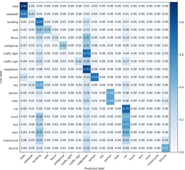
The normalized confusion matrix of the results on this test set with generated labels is on Figure 11. It is apparent that some classes are recognized reasonably well, such as road, building, vegetation, car, person and even bicycle. On the other hand, some classes are often confused for others, for example sidewalk is often labelled as road, walls are labelled as buildings and fences are commonly labelled as vegetation, as well as building or car. Moreover, some classes like traffic light, sky, rider, bus and others are almost never labelled with the correct class. The classes that are recognized better coincide with classes that are well represented in the dataset, such as building, vegetation and car.

The per class metrics are listed in Table 1. The missing entries for some classes are due to no prediction of the class being made. The class accuracies are high, but due to there being multiple classes this value is inflated by the large amount of true negatives.

road

sidewalkbuilding wall fence_{polegrouptraffic lighttraffic signvegetation} terrain skyperson rider car truck bus train_motorcyclebicycle

Predicted label road sidewalk building wall fence polegroup traffic light traffic sign vegetation terrain sky person rider car truck bus train motorcycle bicycle True label 0.92 0.02 0.00 0.00 0.00 0.00 0.00 0.00 0.01 0.03 0.00 0.00 0.00 0.01 0.00 0.00 0.00 0.00 0.00 0.67 0.22 0.01 0.00 0.00 0.00 0.00 0.00 0.03 0.04 0.00 0.00 0.00 0.01 0.00 0.00 0.00 0.00 0.01 0.01 0.01 0.69 0.02 0.00 0.01 0.00 0.00 0.17 0.01 0.00 0.00 0.00 0.07 0.00 0.00 0.00 0.00 0.00 0.02 0.02 0.37 0.33 0.04 0.00 0.00 0.00 0.13 0.01 0.00 0.00 0.00 0.09 0.00 0.00 0.00 0.00 0.00 0.03 0.02 0.19 0.05 0.15 0.01 0.00 0.00 0.37 0.05 0.00 0.00 0.00 0.14 0.00 0.00 0.00 0.00 0.00 0.07 0.03 0.11 0.01 0.01 0.32 0.00 0.01 0.32 0.06 0.00 0.02 0.00 0.05 0.00 0.00 0.00 0.00 0.01 0.01 0.00 0.14 0.00 0.00 0.03 0.00 0.01 0.72 0.01 0.00 0.01 0.00 0.04 0.00 0.00 0.00 0.00 0.03 0.04 0.01 0.21 0.00 0.00 0.03 0.00 0.22 0.26 0.03 0.00 0.02 0.00 0.17 0.00 0.00 0.00 0.00 0.00 0.01 0.00 0.06 0.01 0.01 0.01 0.00 0.00 0.83 0.04 0.00 0.00 0.00 0.03 0.00 0.00 0.00 0.00 0.01 0.15 0.01 0.00 0.00 0.00 0.00 0.00 0.00 0.13 0.69 0.00 0.00 0.00 0.01 0.00 0.00 0.00 0.00 0.00 0.02 0.10 0.49 0.05 0.00 0.00 0.00 0.03 0.15 0.00 0.00 0.00 0.00 0.15 0.00 0.00 0.00 0.00 0.00 0.05 0.02 0.11 0.00 0.00 0.02 0.00 0.01 0.18 0.01 0.00 0.48 0.00 0.08 0.00 0.00 0.00 0.00 0.03 0.02 0.01 0.06 0.00 0.00 0.01 0.00 0.01 0.21 0.01 0.00 0.49 0.00 0.06 0.00 0.00 0.00 0.00 0.12 0.05 0.01 0.05 0.00 0.00 0.00 0.00 0.00 0.11 0.02 0.00 0.00 0.00 0.75 0.00 0.00 0.00 0.00 0.00 0.02 0.00 0.34 0.01 0.00 0.00 0.00 0.00 0.13 0.01 0.00 0.00 0.00 0.47 0.00 0.00 0.00 0.00 0.00 0.01 0.00 0.26 0.00 0.01 0.00 0.00 0.00 0.14 0.01 0.00 0.00 0.00 0.55 0.00 0.00 0.00 0.00 0.00 0.03 0.00 0.37 0.03 0.01 0.00 0.00 0.00 0.11 0.02 0.00 0.00 0.00 0.42 0.00 0.00 0.00 0.00 0.00 0.06 0.03 0.25 0.00 0.00 0.00 0.00 0.01 0.20 0.01 0.00 0.04 0.00 0.25 0.00 0.00 0.00 0.00 0.15 0.04 0.05 0.10 0.00 0.00 0.01 0.00 0.01 0.19 0.02 0.00 0.04 0.00 0.08 0.00 0.00 0.00 0.00 0.47 0.0 0.2 0.4 0.6 0.8

Figure 11. The confusion matrix for the true labels and predicted labels for PointNet++ learning evaluation on generated labels. Normalization is performed row-wise, meaning that the numbers on diagonal represent recall rather than precision.

Table 1. Per class metrics for PointNet++ learning evaluation.

Class Accuracy Recall Precision F1-score IoU Proportion

Road 0.904 0.923 0.852 0.886 0.795 0.403 Sidewalk 0.935 0.215 0.510 0.303 0.178 0.065 Building 0.939 0.692 0.668 0.680 0.515 0.093 Wall 0.988 0.330 0.443 0.378 0.233 0.011 Fence 0.988 0.150 0.373 0.214 0.120 0.011 Polegroup 0.990 0.320 0.432 0.368 0.225 0.010 Traffic light 1.000 0.000 - - 0.000 0.000 Traffic sign 0.996 0.222 0.406 0.287 0.168 0.003 Vegetation 0.907 0.832 0.741 0.734 0.644 0.202 Terrain 0.949 0.689 0.660 0.674 0.508 0.077 Sky 1.000 0.000 - - 0.000 0.000 Person 0.993 0.484 0.670 0.523 0.401 0.010 Rider 1.000 0.000 - - 0.000 0.001 Car 0.950 0.745 0.725 0.735 0.581 0.094 Truck 0.995 0.000 0.000 - 0.000 0.005 Bus 0.999 0.000 - - 0.000 0.001 Train 0.996 0.001 0.493 0.001 0.001 0.004 Motorcycle 1.000 0.000 - - 0.000 0.000 Bicycle 0.993 0.470 0.562 0.512 0.344 0.008

When evaluating recall, precision and F1-score, only three classes have values over 0.7: road, vegetation, car, which are also the three most common classes in the dataset.

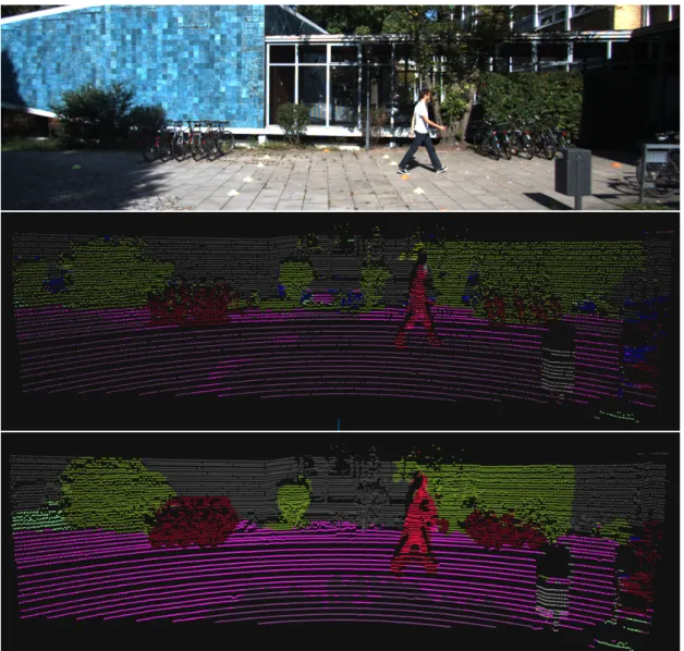
Comparisons between the original image, the projected semantic segmentation labels and the predicted point labels are on Figure 12 and Figure 13. The first depicts a successful labelling, with the person, bicycles and vegetation correctly predicted. The second, however, contains a mislabelling of a walking person in the predicted point labels, but for that scene the projected semantic segmentation is also mislabelled, as the person on the bicycle is labelled as a car and the bicycle itself a person.

Figure 12. Example of successful labelling. Top: camera image, middle: projected labels, bottom: PointNet++ predictions.

Figure 13. Example of mislabelling. The person on the right is labelled as a person (legs), car (torso) and traffic sign (head). Top: camera image, middle: projected labels, bottom: PointNet++ predictions.

4.2

Ground truth evaluation

Following the transformation of ground truth 3D bounding boxes into points, the trained model achieves a pointwise accuracy of 0.498. The normalized confusion matrix between predicted classes and ground truth classes is on Figure 14. In this evaluation task the pedestrian and car classes are detected very well, however the car class makes up for the biggest amount of false positives, i.e. the points that fell outside the bounding boxes. It is also clear that the cyclist class is indeed mostly labelled as a combination of the person and bicycle classes, with the person class constituting 49% of the points that fell inside cyclist object bounding boxes.

road

sidewalk building wall fence _{polegroup traffic sign vegetation} terrain person car truck bicycle

Predicted label Unlabelled Pedestrian Car Cyclist True label 0.00 0.00 0.00 0.00 0.00 0.00 0.00 0.00 0.00 0.03 0.85 0.00 0.12 0.02 0.00 0.03 0.00 0.00 0.03 0.01 0.04 0.00 0.83 0.03 0.00 0.01 0.03 0.00 0.01 0.00 0.00 0.00 0.00 0.03 0.00 0.00 0.92 0.00 0.00 0.03 0.02 0.02 0.00 0.00 0.00 0.01 0.10 0.00 0.49 0.04 0.00 0.28 0.0 0.2 0.4 0.6 0.8

Figure 14. The confusion matrix for the true labels from 3D ground truth and predicted labels. Normalization is performed row-wise.

Table 2. Per class metrics for KITTI ground truth evaluation

Class Accuracy Recall Precision F1-score IoU Proportion

Pedestrian 0.971 0.826 0.666 0.738 0.584 0.050 Car 0.580 0.922 0.543 0.683 0.519 0.492 Cyclist 0.938 0.282 0.063 0.103 0.055 0.013

The per class metrics are listed in Table 2. While accuracy is high for the pedestrian and cyclist classes, it is also inflated due to the large amount of true negatives. Both pedestrian and car classes achieve an F1-score near or over 0.7, with the result for car

being lower due to low precision, even though the recall is higher. As the cyclist ground truth label is predicted as a combination of person and bicycle, the F1-score is low. If similarity between the pointwise intersection over union and KITTI volume-wise intersection over union is assumed, the car score is much lower than the leaderboard top result of 0.776, but the pedestrian score is exceeding the current state-of-the-art with the top result of 0.466 [noad].

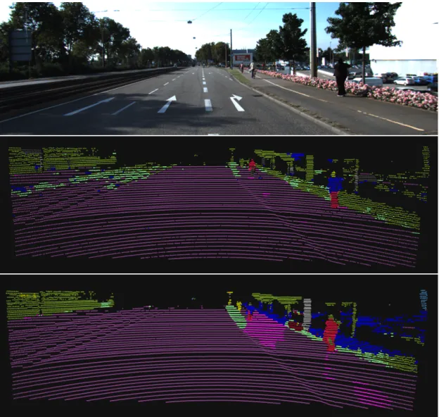
Comparisons between the original image, the projected semantic segmentation labels and the predicted point labels with both of the latter also containing ground truth 3D bounding boxes are on Figure 15 and Figure 16. On the first figure, it can be seen how the person and bicycle points of the cyclist object on the left are labelled separately, but the object can be considered detected. It can also be seen that the projected semantic segmentation labels mislabel two persons on the right, whereas in the predictions these are somewhat correctly labelled. On the second figure, multiple correctly labelled cars can be seen, although some of the wall on the right is also mislabelled as car.

Figure 15. Example of the “cyclist” object on the left being detected correctly, but labelled using person and bicycle classes. The truck in the middle, however, is mislabelled. Top: camera image, middle: projected labels, bottom: PointNet++ predictions.

Figure 16. Example of successful labelling of multiple cars. Top: camera image, middle: projected labels, bottom: PointNet++ predictions.

4.3

Parameter tuning experiments

Results for experiments performed with varying voxel sizes with the number of points kept at the default value of 8192 are in Table 3.

Table 3. Voxel size experiments

Voxel size Best pointwise accuracy

1.5 0.773 3.0 0.797 4.5 0.782 6.0 0.753 7.5 0.722 9.0 0.707

It can be seen the a voxel size of 3 meters performs the best. The most likely explanation for 3.0 meters performing the best is the difference in the used datasets. As the original value of 1.5 meters is chosen using the size of a human, the outdoor dataset also contains objects like cars and trucks, which are better captured when using a larger voxel size. The performance drops from 4.5 meters onwards is likely due to the fact that the sampled voxels are very large and have a lot of empty space in them.

Results for experiments performed with varying number of points with voxel size kept at the default value of 1.5 meters are in Table 4.

Table 4. Number of points experiments

Number of points Best pointwise accuracy

8192 0.773

4096 0.778

2048 0.765

1024 0.746

Of these tested values, the number of points being 4096 performs the best. This is likely due to the fact that the average point density in the used outdoor dataset is smaller

than the original dataset this parameter was used for. While the values 8192 and 4096 perform very closely, the latter is preferable due to slightly faster training.

Combining the best parameter values from the two sets of experiments yields a voxel size of 3.0 meters and 4096 points. The results for additional experiments to study any interactions between the two parameters and to find the best performing model are in Table 5.

Table 5. Combined voxel size and number of points experiments

Voxel size Number of points 8192 4096 2048 1.5 0.773 0.778 0.765 3.0 0.797 0.812 0.786 4.5 0.782 0.776 0.769

From the results it can be seen that there are no unexpected interactions between these parameters and the combination of the two best separately tested parameter values yields the overall best model.

5

Summary

The goal of this work was to validate the approach of using 2D pixel labels to train a model to predict 3D point labels directly from point cloud. For this, a dataset with corresponding images and point clouds was used. The images were first labelled using semantic segmentation network, after which the 2D pixel labels were projected onto 3D points. These labelled points were then used to train a PointNet++ model to predict 3D point labels from only point cloud information. The results were then evaluated on the KITTI dataset ground truth that was generated from 3D bounding box labels.

The model learned to make meaningful predictions despite there being multiple sources of noise in the label generation process. For example, the PointNet++ model managed to correctly predict humans from point cloud data when the semantic segmenta-tion model mislabelled them on the camera image. While the predicsegmenta-tions on the car class lag behind the state-of-the-art in the KITTI dataset, the predictions on the pedestrian class are comparable or even exceeding the state-of-the-art.

The main direction for future experiments is extending the existing pipeline to produce 3D bounding box predictions. For this, the entire field of view from the LiDAR needs to be included, as well as a method to produce the bounding boxes from labelled points. This would allow direct comparison with official KITTI performance metrics. To further improve results for this evaluation, newer network architectures, for example PointPillars[LVC+18], also work on only point cloud data and can be used instead of PointNet++. For additional inputs, the reflectivity data from the LiDAR sensor can be added. In addition, RGB data from cameras could also be added, if reliance on just once sensor is not crucial.

Acknowledgements

I would like to thank Tambet Matiisen for providing me with the chance to work on the cutting edge of autonomous vehicle research and for the constant support in both practical and theoretical tasks. I would also like to thank Milrem Robotics for giving me the opportunity to work on the Nutikas UGV project.

References

[Bar16] Michael Barnard. Tesla & google disagree about LIDAR – which is right? | CleanTechnica. https://cleantechnica.com/2016/07/29/ tesla-google-disagree-lidar-right/, July 2016. Accessed: 2019-5-2.

[CBL+_{19] Holger Caesar, Varun Bankiti, Alex H Lang, Sourabh Vora, Venice Erin}

Liong, Qiang Xu, Anush Krishnan, Yu Pan, Giancarlo Baldan, and Oscar Beijbom. nuscenes: A multimodal dataset for autonomous driving. March 2019.

[Cha17] Ching-Yao Chan. Advancements, prospects, and impacts of automated driving systems, 2017.

[Cho17] Francois Chollet. Xception: Deep learning with depthwise separable convolutions, 2017.

[COR+16] Marius Cordts, Mohamed Omran, Sebastian Ramos, Timo Rehfeld, Markus Enzweiler, Rodrigo Benenson, Uwe Franke, Stefan Roth, and Bernt Schiele. The cityscapes dataset for semantic urban scene understanding, 2016.

[CPK+18] Liang-Chieh Chen, George Papandreou, Iasonas Kokkinos, Kevin Murphy, and Alan L Yuille. DeepLab: Semantic image segmentation with deep convolutional nets, atrous convolution, and fully connected CRFs. IEEE Trans. Pattern Anal. Mach. Intell., 40(4):834–848, April 2018.

[CQCS+_{17] R Qi Charles, R Qi Charles, Hao Su, Mo Kaichun, and Leonidas J Guibas.}

PointNet: Deep learning on point sets for 3D classification and segmenta-tion, 2017.

[CZP+_{18] Liang-Chieh Chen, Yukun Zhu, George Papandreou, Florian Schroff, and}

Hartwig Adam. Encoder-Decoder with atrous separable convolution for semantic image segmentation, 2018.

[DCS+_{17] Angela Dai, Angel X Chang, Manolis Savva, Maciej Halber, Thomas}

Funkhouser, and Matthias NieBner. ScanNet: Richly-Annotated 3D recon-structions of indoor scenes, 2017.

[GLSU13] A Geiger, P Lenz, C Stiller, and R Urtasun. Vision meets robotics: The KITTI dataset, 2013.

[GLU12] A Geiger, P Lenz, and R Urtasun. Are we ready for autonomous driving? the KITTI vision benchmark suite, 2012.

[GMM] S B Goldberg, M W Maimone, and L Matthies. Stereo vision and rover navigation software for planetary exploration.

[HZ03] Richard Hartley and Andrew Zisserman. Multiple View Geometry in Com-puter Vision. Cambridge University Press, 2003.

[HZRS16] Kaiming He, Xiangyu Zhang, Shaoqing Ren, and Jian Sun. Deep residual learning for image recognition, 2016.

[LMB+14] Tsung-Yi Lin, Michael Maire, Serge Belongie, James Hays, Pietro Perona, Deva Ramanan, Piotr Dollár, and C Lawrence Zitnick. Microsoft COCO: Common objects in context, 2014.

[LSD15] Jonathan Long, Evan Shelhamer, and Trevor Darrell. Fully convolutional networks for semantic segmentation, 2015.

[LSG08] Nalpantidis Lazaros, Georgios Christou Sirakoulis, and Antonios Gaster-atos. Review of stereo vision algorithms: From software to hardware, 2008.

[LVC+18] Alex H Lang, Sourabh Vora, Holger Caesar, Lubing Zhou, Jiong Yang, and Oscar Beijbom. PointPillars: Fast encoders for object detection from point clouds. December 2018.

[Mor] Yannick Morvan. multi-view video coding. http://epixea.com/ research/multi-view-coding-thesisch2.html. Accessed: 2019-5-3.

[noaa] Cameras or lasers? https://www.templetons.com/brad/robocars/ cameras-lasers.html. Accessed: 2019-5-3.

[noab] Depth sensing - advanced settings | stereolabs. https://www.stereolabs. com/docs/depth-sensing/advanced-settings/. Accessed: 2019-5-2.

[noac] HDL-64E. https://velodynelidar.com/hdl-64e.html. Accessed: 2019-5-2.

[noad] The KITTI vision benchmark suite.http://www.cvlibs.net/datasets/ kitti/eval_object.php?obj_benchmark=3d. Accessed: 2019-5-12.

[noa18] Rain driving for AI Self-Driving cars - AI trends.https://www.aitrends.

com/ai-insider/rain-driving-ai-self-driving-cars/, January

2018. Accessed: 2019-5-2.

[QYSG17] Charles R Qi, Li Yi, Hao Su, and Leonidas J Guibas. PointNet++: Deep hierarchical feature learning on point sets in a metric space. June 2017.

[RFB15] Olaf Ronneberger, Philipp Fischer, and Thomas Brox. U-Net: Convolu-tional networks for biomedical image segmentation, 2015.

[SMAG19] Martin Simon, Stefan Milz, Karl Amende, and Horst-Michael Gross. Complex-YOLO: An Euler-Region-Proposal for Real-Time 3D object de-tection on point clouds, 2019.

[SWL18] Shaoshuai Shi, Xiaogang Wang, and Hongsheng Li. PointRCNN: 3D object proposal generation and detection from point cloud. December 2018.

[TI] TI. An introduction to automotive LIDAR. http://www.ti.com/lit/wp/ slyy150/slyy150.pdf. Accessed: 2019-5-3.

[YML18] Yan Yan, Yuxing Mao, and Bo Li. SECOND: Sparsely embedded convolu-tional detection. Sensors, 18(10), October 2018.

Appendix

I. Licence

Non-exclusive licence to reproduce thesis and make thesis public

I,Markus Loide,

(author’s name)

1. herewith grant the University of Tartu a free permit (non-exclusive licence) to

reproduce, for the purpose of preservation, including for adding to the DSpace digital archives until the expiry of the term of copyright,

Automatic Labelling of Point Clouds Using Image Semantic Segmentation,

(title of thesis)

supervised by Tambet Matiisen.

(supervisor’s name)

2. I grant the University of Tartu a permit to make the work specified in p. 1 available to the public via the web environment of the University of Tartu, including via the DSpace digital archives, under the Creative Commons licence CC BY NC ND 3.0, which allows, by giving appropriate credit to the author, to reproduce, distribute the work and communicate it to the public, and prohibits the creation of derivative works and any commercial use of the work until the expiry of the term of copyright.

3. I am aware of the fact that the author retains the rights specified in p. 1 and 2.

4. I certify that granting the non-exclusive licence does not infringe other persons’ intellectual property rights or rights arising from the personal data protection legislation.

Markus Loide