Log-skew-normal accelerated failure time models

(1)

Working Paper Series, N. 3, March 2012

Log-skew-normal accelerated failure time models

Andrea Callegaro

Department of Statistical Sciences University of Padua

Italy

Abstract: Accelerated Failure Time models (AFT) are useful alternatives to the Cox model in survival analysis. Recently, AFT models for multivariate data have been considered with flexible distributions of the error term. In this paper, we focus on AFT models with flexible distributions of random effects. In particular, we consider multivariate skew-normally distributed random ef-fects. When the sample size is large, flexible distribution of the random effects provides a better description of the dependence structure on the data. The performance of the model is evaluated by simulations. Further, the proposed log-skew-normal AFT model is illustrated with data on multiple myeloma pa-tients with autologous transplantation from the European Bone Marrow Trans-plantation Registry.

Keywords: Accelerated failure time model, Frailty model, Multivariate Sur-vival analysis, Skewed-normal distribution

(2)

Log-skew-normal accelerated failure time models

Andrea Callegaro

Department of Statistical Sciences University of Padua

Italy

Abstract: Accelerated Failure Time models (AFT) are useful alternatives to the Cox model in survival analysis. Recently, AFT models for multivariate data have been consid-ered with flexible distributions of the error term. In this paper, we focus on AFT models with flexible distributions of random effects. In particular, we consider multivariate skew-normally distributed random effects. When the sample size is large, flexible distribution of the random effects provides a better description of the dependence structure on the data. The performance of the model is evaluated by simulations. Further, the proposed log-skew-normal AFT model is illustrated with data on multiple myeloma patients with autologous transplantation from the European Bone Marrow Transplantation Registry.

Keywords: Accelerated failure time model, Frailty model, Multivariate Survival analysis, Skewed-normal distribution

The Cox proportional hazards (PH) model (Cox, 1972) is now the most widely used method for the analysis of survival data in the presence of covariates. On the other hand, the Accelerated Failure Time model (AFT) has seldom been utilized in the analysis of censored survival data. However, the AFT model is a useful alternative to the Cox regression model in survival analysis for several reasons. First, results have an intuitive physical interpretation (Wei, 1992). Second, fixed effect parameters are robust toward neglected covariates (Hougaard, 1999). Finally, AFT models should lead to more efficient parameter estimates than the Cox model under certain circumstances (Cox, 1984).

AFT models can be rewritten specifying a direct relation between the logarithm of the survival time and the explanatory variables, just as a multiple linear regression model does. A parametric AFT model assumes that the error term of this linear regression follows a distribution of a specific type (e.g., normal, logistic or Gumbel). In contrast, semi-parametric procedures for the AFT model leave the density of the error term unspecified and provide only the estimate of the regression parameters (Kalbfleish and Prentice, 2002). Evidently, parametric AFT models can fit badly in the case of an incorrect specification of the distribution. Estimates of the re-gression parameters (with the exception of the intercept and the scale parameter) are consistent, but some loss in efficiency is due to an incorrect assumption about the error. In order to achieve more robustness, it is possible to considered a more flexible parametric model, such as the generalized gamma, or the generalized F.

(4)

distribution of the error term given by the skew-normal (SN) distribution (Azzalini, 1985). The SN distribution is an extension of the normal distribution allowing for non-zero skewness by means of a shape parameter. In recent years, this distribution, in its univariate and multivariate version, has received considerable attention both in theoretical studies, for its numerous stochastic properties, and in applied studies, for the additional flexibility that it provides (Azzalini, 2005).

In the second part of the paper, multivariate survival data are considered. AFT models have been widely used in univariate analysis (Kalbfleish and Prentice, 2002), while multivariate life-time models have received less attention. There has been a strong emphasis on semiparametric Cox PH models with random effects (frailties) (Clayton, 1978; Yashin et al., 1995; McGilchrist & Aisbett, 1991), but there has been little discussion of parametric families. Anderson et al. (1995) proposed a model for bivariate survival data with a parametric or non-parametric frailty distribution. Klein et al. (1999) derived a marginal-likelihood approach from a multivariate nor-mal regression model, and Pan (2001) considered AFT models with gamma frailty. More recently, in order to improve the fit, Kom´arek et al. (2005), Kom´arek & Lesaf-fre (2006) and Lambert et al. (2004) have focused on multivariate AFT models with flexible distributions of the error term. In this paper, instead, we focus on flexible distributions of the random effects. We assume that the random effects are multi-variate skew-normal distributed (Azzalini & Dalla Valle, 1996; Azzalini & Capitanio, 1999; Azzalini, 2005) and we show that flexible random effects models are of crucial importance to describe the dependence structure present in the data.

The paper is organized as follows. Sections 2.1 and 2.2 introduce the skew-normal distribution and the AFT models, respectively. In Section 2.3 we derive a univariate model with skew-normal error terms. In Section 2.4 a multivariate AFT model with skew-normal random effects is proposed. The marginal likelihood is derived for the case when the error term is normal. An approximated likelihood approach is proposed for maximum likelihood estimation. Section 3.1 presents the simulation results. In Section 3.2 the proposed new method is illustrated by an application to a real data set of multiple myeloma patients with autologous transplantation from the European Bone Marrow Transplantation Registry. Finally, Section 4 presents a discussion of the proposed models.

1 Methods

1.1 Skew-normal distribution

The skew-normal (SN) distribution is an extension of the normal distribution to allow for non-zero skewness (Azzalini, 1985). In the one-dimensional case, the density with locationξ, scaleω and shape parameterα (ξ, α∈R, ω∈R+) is given by

f(x, ξ, ω2, α) = 2ω−1φ($)Φ(α$), (1) where$= (x−ξ)/ω,φand Φ denote the N(0,1) density and distribution function, respectively. When α = 0, the density corresponds to the normal density. The distribution is right skewed ifα > 0 and it is left skewed ifα < 0. An alternative parametrization of the SN distribution can be derived in terms of the mean µ,

(5)

Section 1 Methods 3

the standard deviation σ and the Pearson’s index of skewness γ1 of X. We denote (µ, σ2_{, γ}

1) as the “centred parameters” (CP) while the parameters (ξ,Ω, α) are called direct (DP) because they can be read directly from (1). We will adopt the notation X∼SNDP(ξ, ω2, α) if the density is expressed in terms of the direct parameters, and X∼SNCP(µ, σ2, γ1) if the density is expressed in terms of the centred parameters. The multivariate SN distribution with location ξ, scale Ω, and shape parameter α is given by Azzalini & Capitanio (1999):

f(x, ξ,Ω, α) = 2φd(x−ξ; Ω)Φ(αTω−1(x−ξ)), (2)

where x ∈ Rd_, _α _{is the shape parameter (α} _∈ _Rd_{), and} _ω _{is the diagonal matrix} formed by the standard deviations of Ω. If a d-dimensional variableX has density (2), we say that its distribution is multivariate SN and write Y ∼ SNDP(ξ,Ω, α). The distribution can be expressed in terms of the centered parametrization Y ∼

SNCP(µ,Σ, γ1) whereµ is the mean, Σ is the variance-covariance matrix and γ1 is the multivariate index of skewness of X. For statistical inference it is known that centred parametrization provides a more convenient parametrization than the direct parametrization which is commonly employed for writing the density (Arellano et al., 2008).

1.2 Accelerated Failure Time (AFT) models

The AFT model can be written as being log-linear with respect to time, giving

ln(Tj) =X_jTβ+ωeej, (3)

where Tj and Xj denote the event time and the vector of covariates measured for thej-th individual, respectively. ωe denotes the scale parameter andej the random error term for the j-th individual. The interpretation of model (3) is straightfor-ward: the survival times are multiplied by a constant effect, and the exponentiated coefficients, exp(βk), represents time ratios. The interpretation of the parameters differs crucially from the interpretation of the parameters estimated by the propor-tional hazard model, where exp(βk) represents hazard ratios. Only in the particular case that the survival times follow a Weibull distribution, it can be shown that the AFT and proportional hazard models are the same. The error terms are usually assumed to follow a specific distributional form (normal, logistic, or Gumbel). Al-ternative methods include semiparametric AFT models, in which the distribution of the error term is estimated nonparametrically (Kalbfleish and Prentice, 2002). The log-likelihood function may be written as

`(β, ωe) = n X

j=1

dj(−lnωe+ lnfe($j)) + (1−dj) lnSe($j), (4)

where dj is the indicator of whether the j-th failure time is observed (dj = 1) or is right censored (dj = 0), $j = (lntj −Xjβ)/ωe, and Se(x) = R_x∞fe(u)du is the survival function of the error term.

(6)

For multivariate data, the accelerated failure time models have been extended to include random effects

ln(Tij) =XijTβ+ZijTbi+ωeeij, (5) with Tij the event time for subject j from cluster i, Xij the vector of covariates for subject j from cluster i, β the vector containing the covariate effects, bi the random effect for cluster i, Zij the known design vector for the random effects, ωe the scale parameter, and finallyeij the random error term for subjectjfrom cluster i. Different distributional assumptions have been proposed for the random effects and for the error term (Klein et al., 1999; Pan, 2001; Chang, 2004; Kom´arek et al., 2005; Kom´arek & Lesaffre, 2006; Lambert et al., 2004).

1.3 Univariate log-skew-normal AFT

Let us consider the univariate AFT model (3) where the error term ej follows a skew-normal distribution with null location, unit scale, and shape parameter αe, ej ∼SNDP(0,1, αe), then

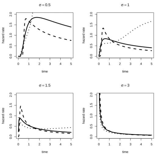
Yj = lnTj ∼SNDP(X_jTβ, ω2_e, αe). (6) The density and the survival function of the error term are fe($) = 2φ($)Φ(αe$) and Se($) = 1 −Φ($) + 2OT($, αe), respectively, where OT is the Owen’s T function and $ = (lnt−XTβ)/ωe. The corresponding hazard rate is given by λ(t, β, ωe, αe) =fe($)/(tωeSe($)). Figure 1 shows the hazard function of the log-skew-normal distribution with different values of skewness parameter. As expected, the additional skewness parameter changes the shape of the hazard function consid-erably.

The log-likelihood is given by equation (4). Maximum likelihood methods can be employed to estimate the parameters of the distribution. A peculiar aspect of the skew-normal log-likelihood function is that, for small/moderate sample size, it can be monotone inαe. To solve this problem we propose a penalize likelihood approach (see Appendix A for details). The performance of the penalized approach will be evaluated by simulations.

An alternative univariate model can be obtained assuming a null mean error termej ∼ SNCP(0,1, γ1e). An advantage of this null mean model with respect to the null location model of equation (6) is that the parameters β and ωe have the same interpretation as the parameters estimated by the classical log-normal AFT model.

1.4 Multivariate log-skew-normal AFT

Let us consider the multivariate AFT model (5) where the random effectbi is mul-tivariate skew-normal distributed bi ∼SNCP(0,Σb, γ1,b). The log-likelihood of the i-th cluster conditional on the random effects bi can be expressed by

`C_i (β, ωe|bi) = ni

X

j=1

(7)

Section 1 Methods 5

where$ij = log(tij)−Xijβ−Z T ijbi

ωe and Se(x) =

R∞

x fe(u)du. The marginal likelihood is then L(θ) = G Y i=1 Z exp{`C_i (β, ωe|bi) + logfb(bi)}dbi. (7)

Note that different distributions of the error term (extreme value, normal, skew-normal, logistic) can be combined with skew normal random effects. For example, if the error term follows a standard type I extreme value (Gumbel) distribution, then fe(x) = exp(x−exp(x)) and Se(x) = exp(−exp(x)). If the error term follows a logistic distribution, thenfe(x) = exp(x)(1 + exp(x))−2 andSe(x) = (1 + exp(x))−1. If the error term is normally distributed: eij ∼ N(0,1), then fe(x) = φ(x) and Se(x) = 1−Φ(x). In this case Y follows a skew normal distribution: Y ∼ SNDP,n(ξ,Ω, α). The contribution to the likelihood of a group where all failure times are observed (n=nD) is the joint density function of equation (2). If there are any censored observations among the nindividuals, then rewrite Y = (YC, YD), where YD is the vector of the (log-transformed) failure times and YD is the vector of the censored failure times. The contribution to the marginal likelihood is the product of the (marginal) density of YD times the conditional survival function of YC givenYD evaluated aty. In this case, the contribution to the likelihood for this group is given by L(θ) =φnD(yD−ξD,ΩD) Z ∞ $∗_C_·_D φnC+1(u,Ω¯ ∗ C·D)du.

All of the parameters (ξ,Ω, α, ξD,ΩD, $∗C·D,Ω¯∗C·D) are derived in Appendix B . The derived marginal likelihood is an extension of the marginal likelihood proposed by Klein et al. (1999) for normal random effects and normal error terms. In appendix B the marginal likelihood is also derived in the case that random effects are Gaussian and the error terms are skew normally distributed.

If the error term is not normal, then it is more complex to derive the marginal likelihood (7). It is, however, possible to approximate the likelihood by numerical methods or Monte Carlo simulation. In this paper, we use a Gaussian quadrature method with 100 nodes. The parameters are estimated maximizing the approxi-mated likelihood. In order to speed up the estimation we propose a two-step proce-dure. In the first step of the procedure, all of the parameters, with the exception of the skewness parameters, are estimated assuming normal distributed random effects. In the second step, the approximated marginal likelihood is maximized with respect to the skewness parameters, with all the other parameters fixed at the values esti-mated at the first step. Standard software can be used to estimate the parameters at the first step. In particular, penalized likelihood approaches (Therneau et al., 2003) implemented in the R package are particularly fast and efficient. The performance of the two-step (fast) procedure will be evaluated by simulations. Standard errors for the estimates will be computed by inverting the Hessian matrix of the approximated likelihood.

(8)

expec-tations of the random effects E{bi}=

R

biexp[`C_i + logfb(bi)]dbi R

exp[`C_i + logfb(bi)]dbi .

The integral can be approximated by numerical methods or Monte Carlo simulations. Prediction is beyond the scope of this paper and will not be further considered.

1.4.1 Shared AFT model

In this section we study the relation between the skewness of the random effects and the dependence structure of the data. To simplify the exposition, we consider the bivariate case (nj = 2) with shared random effects:

ln(Tij) =Yij =XijTβ+bi+ωeeij, (8) wherebi ∼SNCP(0, σ2b, γ1,b) is the null mean random effect with standard deviation σb and the Pearson index of skewness is given byγ1,b,i= 1, ..., Gand j= 1,2.

If the error term is normal, eij ∼ N(0,1), then parameters are easily inter-pretable. In fact,E{Yij}=X_ijTβ; var{Yij}=σ2_b+ω_e2, and cov{Yik, Yil}=σ2_b,k6=l. The correlation between the log-survival times of any two members of a group is ρ=σ_b2/(σ2_b +ω2_e).

A classical measure of local dependence is given by the cross-ratio function (Clay-ton, 1978). The cross-ratio function can be expressed as the ratio of two hazards, i.e., the ratio of the hazard of subject j given that subject l “died” at tl and the hazard ofj given thatTl> tl.

CR(t1, t2) = λ(t1|T2 =t2) λ(t1|T2 > t2) = S(t1, t2)D1D2S(t1, t2) D1S(t1, t2)D2S(t1, t2), (9) whereDj = _∂t∂

j and, in an obvious notation, S(t1, t2) =

Z ∞ −∞

Se($1)Se($2)fb(u)du.

denotes the marginal bivariate survival function, with$j = (yj−XjTβ−u)/ωe. In our case, the marginal survival function does not have a closed form, and we use Gaussian quadrature to approximate it.

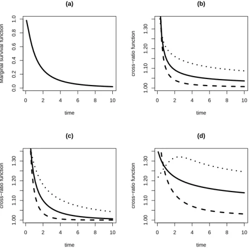
Figure 2 shows the marginal survival function and the cross-ratio functionCR(t, t) for the bivariate log-skew-normal AFT model (8) with three different values of the skewness parameter γ1,b = −0.9, 0, and 0.9, respectively. Figure 2(a) shows the marginal survival function of the log-normal AFT model with normal error terms, β = 0, σb = 0.5, and ωe = 1. Figure 2(b) shows the cross-ration function of the model with normal error terms. If γ1,b is null, this model corresponds to the mul-tivariate log-normal AFT model proposed by Klein et al. (1999). The dependence induced by this model is a function that decreases over time. When γ1,b is nega-tive (posinega-tive), the dependence decreases over time at a smaller (higher) rate with respect to the log-normal model. Figure 2(c) shows the cross-ratio function of the

(9)

Section 2 Results 7

model with logistic error terms. The dependence induced by this model is qualita-tively similar to the dependence structure induced by the model with normal error terms. Finally, Figure 2(d) shows the cross-ratio function of the model with extreme value distributed error terms. Interestingly, in this case the skew parameter has a strong effect on the dependence structure. When the skew parameter is negative, the cross-ratio function increases at the beginning of the follow-up, and then it decreases slowly over time.

2 Results

2.1 Simulation study

Two numerical studies, based upon 500 replications of simulated data, are presented to evaluate the performance of the proposed estimation procedures.

First, we consider the univariate case. The log-transformed survival times Yj were generated using a skew-normal distributionSNCP(µj, ω_e2, γ1,e) with µj =β0+ β1xj,β0= 5,β1 = 0.3 andxj ∼N(0,1). The corresponding censoring timesCj were generated from a uniform distribution between infinity and a lower limit determined in order to achieve approximately the right censoring rate around 30%. Data were simulated with ωe = 1 and skewness parameters γ1,e equal to -0.9, 0 or 0.9. We considered a sample size ofn= 200. Table 1 shows the results of the univariate log-skew-normal AFT method with penalized likelihood (as described in Appendix A ). The penalty avoids infinity estimates of the shape parameter, with a very small bias. As a comparison, we also fitted the classical log-normal AFT model usingsurvreg in the survival package in R. As expected, when the shape parameter differs from zero, the proposed model outperforms the log-normal AFT model.

Secondly, we investigate the performance of the multivariate skew-normal AFT model. The log-transformed survival timesYij, conditioned on the random intercept bi, were generated using a normal distributionN(µij+bi, ω2_e) withµij =β0+β1xij, β0 = 5, β1 = 0.3, xij ∼ N(0,1). The random intercept was skew-normally dis-tributed bi ∼SN(0, σb2, γ1,b) with σb = 0.5 and skew parameters γ1,b =−0.9, 0, or 0.9. We considered G = 200 clusters with ni = 10 subjects in each cluster. The corresponding censoring times Cij were generated from a uniform distribution be-tween infinity and a lower limit determined in order to achieve approximately the right censoring rate around 30%. Table 2 shows the parameters estimated by the two-step (fast) version of the maximum likelihood estimation approach. In the first step we estimated ( ˜β,ω˜e,σ˜b) usingsurvregin the R survival package with Gaussian frailties and Gaussian errors. In the second step, γ1,b was estimated by maximiz-ing the approximated marginal likelihood (7) with fixed ( ˜β,ωe,˜ σ˜b). Integrals were computed by means of Gaussian quadrature with 100 nodes. First, note that the parameters estimated by the penalized likelihood (Therneau et al., 2003) approach are slightly biased. In particular, ωe is underestimated, irrespectively of the skew parameter. A different method (software) could be used in the first step. Second, note that the estimated skew-parameter is biased toward zero however, even in the presence of this bias, the power to detect skewed random effects at the level of 5% is about 80%. Finally, note that with this sample size the approximated log-likelihood

(10)

is not monotone inγ1,b (data not shown).

2.2 Application to multiple myeloma patients with autologous

trans-plantation

We applied the proposed skew-normal AFT model to a real data set from the Eu-ropean Group for Blood and Marrow Transplantation (EBMT) registry. Multiple Myeloma (MM) patients with autologous transplantation were considered. The orig-inal MM autologous registry includes about 52,000 cases. As an illustration, in this analysis we considered only a subset of 3,081 patients i) with common myelo-mas (IgA, IgG), ii) transplanted after 1998, and iii) without inconsistent records or missing values in a list of relevant prognostic factors. Since missing data may be centre/patient-related, with potential patterns of selection bias, this application is not meant to reach conclusions relevant to clinical knowledge or practice.

Patients are clustered into G =190 centres with a mean of 16 individuals per cluster (median 7, minimum=1, maximum=134). We studied Progression Free Sur-vival (PFS), where the failure time is defined as the time from autologous trans-plantation to any of the three following events: a) disease progression, b) disease relapse/recurrence (for patients transplanted in Complete Remission (CR) or achiev-ing CR later on), and c) death without relapse/progression. The number of observed events is 1,548 (51%), and the median PFS time is 14.85 months (minimum=0.03, maximum=119.18). We considered the following risk factors: year of the transplant (from 1999 to 2009), gender (female 42% versus male 58%), stage at diagnosis (I 16%, II 26%, and III 58%), disease status at conditioning (no complete remission 89% versus complete remission 11%), serum beta(2)-microglobulin level at diagnosis (31%>4 versus 69%≤4), the interval between diagnosis and the first transplant in years (median 0.6, minimum=0.003, maximum=17.8), and age at transplant (me-dian 58.4, minimum=20, maximum=78.9).

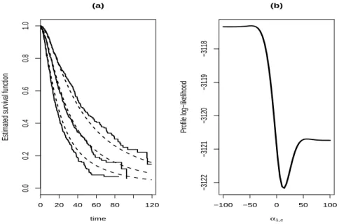
Initially, different models were fit without random effects, in order to identify the distribution of the error term. The failure times were modelled using Weibull, log-logistic, log-normal and log-skew-normal distributions. No skewness was detected by the skew-normal AFT model, and the likelihood value of the Weibull, log-normal, and log-logistic AFT model were -3204.4, -3191.9, and -3163.7, respectively. Based on the AIC criterion, we selected the log-logistic model. To check the model adequacy, we stratified the linear predictor valuesX_jTβˆ into seven categories. The estimated survivor functions were computed for each patient and averaged within each stratum. Figure 3(a) shows the fitted survival functions and the Kaplan-Meier estimates for the first, fourth, and seventh strata of the skew-normal AFT model. The data are fit reasonably well by the considered model, especially before 30 months of follow-up, where most of the observed events are concentrated.

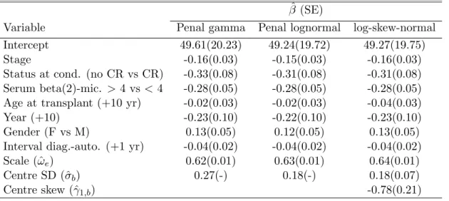
Secondly, we performed a multivariate analysis where centre effects were mod-elled through a shared random effect. We fitted a shared AFT model with skew-normal random effects and logistic error terms (see the third column of Table 3). The estimated skew parameter is -0.78 (se= 0.21). Both Wald type and likelihood ratio tests indicates that the centre effect is negatively skewed. Further, we fitted the penalized method of Therneau et al. (2003) with logistic error term and log-normal

(11)

Section 3 Discussion 9

(penalized log-likelihood value= -7442.25) or gamma distributed frailties (penalized log-likelihood value= -7418.25) (see the first two columns of Table 3). The great difference in the values of the two penalized likelihoods confirms what was detected by the proposed model. Further, it is interesting to note that the frailty distribution has little or no effect on the estimates of the fixed effects (see Table 3).

Finally, we extended the model by including the country effect. Centres are clustered into 26 countries, with a mean of 118 centres per country (median 30, minimum=1, maximum=690). The log-transformed PFS time was modelled by

Ykij =XkijT β+aki+ck+ωeekij, (10) where the centre random effect aki ∼ SNCP(0, σa, γ1,a) was independent of the country random effectck ∼SNCP(0, σc, γ1,c),k= 1, ...,26. The error termekij was assumed to be logistic distributed. Note that model (10) is slightly different from the general model discussed in Section 2.4. In fact, the sum of two independent skew-normal random variables is not generally skew-skew-normal. The marginal likelihood was approximated using Gaussian quadrature, with 100 nodes for each random effect. The estimated parameters of the random effects are (ˆσc,γˆ1,c) = (0.27,−0.99) and (ˆσa,ˆγ1,a) = (0.19,−0.60). The other estimated parameters are substantially un-changed with respect to the model without country effects. Both random effects are significant and left skewed. Figure 3(b) shows the approximated profile log-likelihood of the shape parameter α1,c (which is just a reparametrization of γ1,c). It is evident from the profile log-likelihood that the shape parameter is significantly different from zero, so the dependence due to the country effect is slowly decreasing over time, as shown in Figure 2(c).

3 Discussion

In this paper, we have described accelerated failure time models with skew-normal distributed (Azzalini, 1985) random effects and/or error terms.

For univariate data, the model is an extension of the lognormal AFT model, with an additional parameter to allow for non-zero skewness of the error term. In order to prevent bias of the shape parameter, we proposed a penalized likelihood approach. Simulation results show that, in the presence of skewed error terms, the proposed model outperforms the classical log-normal AFT model.

For multivariate data, we considered log-linear regression models with multivari-ate skew-normal (Azzalini & Dalla Valle, 1996) random effects and general distri-bution of the error terms. We derived the marginal likelihood for the model with normal error terms and we studied the effect of the skewness on bivariate survival times with shared random effects. We showed that the skewness parameter qual-itatively changes the cross-ratio function. It follows that the proposed model is useful to better understand the dependence structure between multivariate failure times. To estimate the parameters, we proposed to maximize the marginal likelihood approximated through Gaussian quadrature. In order to speed up the estimation procedure we developed a two-step procedure where at the first step parameters are estimated assuming Gaussian random effects. Simulation results showed good

(12)

performance of this approach. As illustration, we analyzed a real data of multiple myeloma patients with autologous transplantation. We fitted a hierarchical AFT model with logistic error terms and skew normal centres nested within skew normal countries. Both random effects were negatively skewed, confirming the usefulness of the proposed model.

Recent literature (Kom´arek et al., 2005; Kom´arek & Lesaffre, 2006; Lambert et al., 2004) has emphasized the fact that often the choice of the distribution of the random effect is not important. This is true for small/moderate sample sizes. On the other hand, for large samples, AFT models with flexible distribution of the random effects are crucial to arrive at a good description of the dependence structure present in the data.

The R code used in this paper is available upon request to the author.

Appendix

Appendix A: bias correction for the shape parameter αe

In order to solve the problem of the monotone likelihood inαe, we propose a penal-ized likelihood approach

`(θ)∗=`(θ) +1 2ln[− ∂2`(θ) ∂α2 e ],

where `(θ) is given by Equation (4) with fe($) = 2φ($)Φ(αe$) and Se($) = 1−Φ($) + 2OT($, αe). This approach is similar in spirit to the Firth’s method for bias prevention (Firth, 1993) in generalized linear models. Sartori (2006) proposed to use Firth’s correction for the shape parameter of the scalar skew-normal distribution. Appendix B: marginal likelihood derivation when the error term is normal LetYi = ln(Ti) be a (ni×1) vector of the log-transformed times of thei-th cluster, i= 1, ..., m

Yi =Xiβ+Zibi+ei,

wherebi ∼SNq,DP(0,Ωb, αb) andei ∼Nn(0,Ωei). For the skew-normal distribution we use the parametrization proposed by Azzalini & Capitanio (1999). It follows that

Yi|bi ∼Nni,DP(Xiβ+Zibi,Ωei), bi ∼SNq,DP(0,Ωb, αb).

The sum of a multivariate SN variate and an independent multivariate normal variate isYi∼SNn(ξi,Ωi, αi), whereξi=Xiβ, Ωi =ZiΩbZ_iT + Ωei and

αi = ωiΩi

−1_BT i αb

(1 +αT_b( ¯Ωb−BiΩ_i−1B_iT)αb)1/2 Bi =ω_b−1ΩbZ_iT.

(see Appendix C). In Appendix C,αi is also derived for the case whenbi∼Nq(0,Ωb) andei ∼Nn(0,Ωei, αei).

(13)

Section 3 Discussion 11

In the following, for ease of notation, the subscriptiis omitted. Letd=Pn k=1dk be the number of observed failure times in the group. If there are censored obser-vations among the n individuals, then rewrite Y = (YD, YC), where YD is the d-dimensional vector of the log death times andYC is then−d-dimensional vector of censored observations. The contribution to the likelihood for the group of n obser-vations is the product of the density function for YD times the conditional survival function of YC, given YD evaluated atyD = ln[tD].

First of all, we consider the contribution of the nobserved failure times. Their marginal distribution is YD ∼ SNnD,DP(ξD,ΩDD, αD(C)), so their contribution to the likelihood is

LD = 2φd(yD−ξD; ΩDD)Φ(τC·D),

whereτC·D =αT_D(C)ω_D−1(yD−ξD), with ¯ΩCC·D = ¯ΩCC−ΩCD¯ Ω¯_DD−1 ΩDC¯ andαD(C) = (αD + ¯Ω−_DD1 ΩDCαC)(1 +¯ αT_CΩCC¯ ·DαC)−1/2, which is the shape parameter of the

marginal distribution ofYD.

Now we consider the contribution to the likelihood of the censored observations. The conditional distribution of YC|YD ∼ SNn−d,DP(ξC·D,ΩCC·D, αC·D, τC·D) is an extension of the classical skew normal distribution with an additional parameter (τ_C_·_D). The multivariate survival function of this conditional distribution is given by Capitanio et al. (2003) LC =P(YC ≥yC|YD =yD) = 1 Φ(τC·D) Z ∞ $∗ C·D φn−d+1(u,Ω¯∗CC·D)du, where ¯ Ω∗_CC·D = 1 −˜δT_C_·_D −δ˜C·D Ω˜CC·D , ˜

ΩCC·D = ˜ω−C1·DΩ¯CC·Dω˜−C·1D is the correlation matrix associated to ¯ΩCC·D and ˜

δC·D = ˜ΩCC·DαC·D/(1 +αTC·DΩ˜CC·DαC·D)1/2 $∗_C_·_D = (τC·D,(yC−ξC·D)˜ω_C−·1D)

T_.

The log-likelihood is given by the sum of the contributions of themindependent clusters:

`= m X

i=1

logLD,i+ logLC,i.

If random effects are assumed to have zero means, then the location parameter of Yi becomesξi =X_iTβ−p2/πδ, with δ= ¯Ωα(1 +αTΩα)¯ −1/2.

Appendix C: derivation of the multivariate α

The sum of a multivariate SN variate and a multivariate normal variate is SN. This can be easily seen using the moment generating function. The cumulant generating function of the SN b∼SNq,DP(0,Ωb, αb) is Kb(ti) = 1 2t T_Ω bt+ζ0(δbTωbt),

(14)

where

δb = ¯Ωbαb(1 +αbTΩ¯bαb)−1/2. The cumulant generating function ofe∼Nn(0,Ωe) is

Ke(ti) = 1 2t

T_Ω et.

The cumulant generating function ofY =Zb+e, is given by KY(ti) =

1 2t

T_Ωt₊_ζ

0(δbTωbZTt),

where Ω = ZΩbZT + Ωe. It follows that the distribution is still SN with δTω = δ_bTωbZT, so δT = δbTωbZTω−1. Further, using the following relations α = (1− δTΩδ)¯ −1/2Ω¯−1δ and δb = (1 +αTbΩ¯bαb)−1/2Ω¯bαb, then

α= ωΩ

−1_BT_αb

(1 +αT_b( ¯Ωb−BΩ−1_BT_)αb)1/2 B =ω−_b1ΩbZT.

If we assume that the residual term is skewedb∼Nq(0,Ωb) ande∼SNn,DP(0,Ωe, αe), thenY ∼SNn,DP(ξ,Ω, α), with α= ωΩ −1_BT_αe (1 +αT e( ¯Ωe−BΩ−1BT)αe)1/2 B =ω_e−1Ωe.

References

Anderson, J. E., Louis, T. A. (1995). Survival analysis using a scale change random effects model Journal of the American Statistical Association, 90:669 – 679. Arellano-Valle, R. B., Azzalini, A. (2008). The centred parametrization for the

multivariate skew-normal distribution Journal of Multivariate Analysis, 99:1362– 1382.

Azzalini, A. (1985). A class of distributions which includes the normal ones. Scan-dinavian Journal of Statistics, 12:171–178.

Azzalini, A. (2005). The skew-normal distribution and related multivariate families. Scandinavian Journal of Statistics, 32:159–188.

Azzalini, A. & Capitanio, A. (1999). Statistical applications of the multivariate skew normal distribution. Journal of the Royal Statistical Society, ser. B, 61(3):579– 602. Full version of the paper at arXiv.org:0911.2093.

Azzalini, A. & Dalla Valle, A. (1996). The multivariate skew-normal distribution. Biometrika, 83:715–726.

(15)

REFERENCES 13

Balakrishnan, N., Peng, Y. (2006). Generalized gamma frailty model. Statistics in Medicine, 25:2797–2816.

Capitanio, A., Azzalini, A., Stanghellini E. (2003). Graphical models for skew normal variates. Scandinavian Journal of Statistics, 30:129–144.

Chang, S. (2004). Estimating marginal effects in accelerated failure time models for serial sojourn times among repeated events. Lifetime Data Analysis, 10:175–190. Clayton, D. G. (1978). A model for association in bivariate life tables and its appli-cation in epidemiologic studies of familial tendency in chronic disease incidence. Biometrika, 65:141–151.

Cox, D. R. (1972). Regression models and life tables.Journal of the Royal Statistical Society, B 34:187–220.

Cox, D. R., Oakes, D. Analysis of Survival Data Chapman and Hall, London, 1984. Dempster, A.P., Laird, N.M., and Rubin, D.B. (1977). Maximum likelihood from incomplete data via the EM algorithm (with discussion). Journal of the Royal Statistical Society Ser. B-Stat. Methodol., 39:1–38

Firth, D. (1993). Bias reduction of maximum likelihood estimates. Biometrika, 80: 27–38.

Hougaard, P. (1999) Fundamentals of survival data. Biometrics, 55:13–22.

Kalbfleish,J. D., and Prentice, R. L. (2002) The Statistical Analysis of Failure Time Data 2nd ed. Wiley, New York. 2002, MR1924807

Klein, J. P., Pelz, C., and Zhang, M. (1999) Modeling random effects for censored data by a multivariate normal regression model. Biometrics, 55: 497–506. Kom´arek, A. and Lesaffre, E. (2006). Bayesian semi-parametric accelerated failure

time model for paired doubly interval-censored data. Statistical Modelling, 6: 3–22.

Kom´arek, A., Lesaffre, E. and Hilton, J.F. (2005). Accelerated failure time model for arbitrarily censored data with smoothed error distribution. Journal of Com-putational and Graphical Statistics, 14:726–745.

Lambert, P., Collett, D., Kimber, A., and Johnson, R. (2004). Parametric ac-celerated failure time models with random eects and an application to kidney transplant survival. Statistics in Medicine, 23: 3177–3192.

McGilchrist, C. A., and Aisbett, C. W. (1991). Regression with frailty in survival analysis. Biometrics, 47:461–466.

Pan, W. (2001). Using frailties in the accelerated failure time model. Lifetime Data Analysis, 7:55–64.

(16)

Sartori, N. (2006). Bias prevention of maximum likelihood estimates: skew normal and skew-t distributions.Journal of Statisitical Planning and Inference, 136:4259– 4275.

Therneau, T. M., Grambsch, P. M., and Pankratz, V. S. (2003). Penalized survival models and frailty. Journal of Computational and Graphical Statistics, 156–175. DOI: 10.1198/1061860031365

Wei, L. J. (1992). The accelerated failure time model: a useful alternative to the Cox regression model in survival analysis. Statistics in Medicine, 11:1871–1879. Yashin, A. I., Vaupel, J. W., and Iachine, I. A. (1995). Correlated individual frailty:

An advantageous approach to survival analysis of bivariate data. Mathematical population studies, 5:145–159.

(17)

REFERENCES 15 0 1 2 3 4 5 0.0 0.5 1.0 1.5 2.0 σ =0.5 time hazard r ate 0 1 2 3 4 5 0.0 0.5 1.0 1.5 2.0 σ =1 time hazard r ate 0 1 2 3 4 5 0.0 0.5 1.0 1.5 2.0 σ =1.5 time hazard r ate 0 1 2 3 4 5 0.0 0.5 1.0 1.5 2.0 σ =3 time hazard r ate

Figure 1: Log-skew-normal hazard function with mean µ = 0, and different values of standard deviation σ and skewnessγ1. Straight, dotted and dashed lines denote the hazard function withγ1= 0, -0.9, and 0.9, respectively.

(18)

0 2 4 6 8 10 0.0 0.2 0.4 0.6 0.8 1.0 (a) time Marginal sur viv al function 0 2 4 6 8 10 1.00 1.10 1.20 1.30 (b) time cross−r atio function 0 2 4 6 8 10 1.00 1.10 1.20 1.30 (c) time cross−r atio function 0 2 4 6 8 10 1.00 1.10 1.20 1.30 (d) time cross−r atio function

Figure 2: Cross-ratio function of bivariate AFT models with skew-normal random effect and different distributions of the error term. Figure (a): marginal survival function with normal error term andβ0= (0,0)T,σb = 0.5,ωe= 1. Figures (b), (c), and (d) show the cross-ratio functionsCR(t, t) with error term following the normal, the logistic, and the extreme value distribution, respectively. Straight, dotted, and dashed lines denote the cross-ratio function withγ1,b= 0, -0.9, and 0.9, respectively.

(19)

REFERENCES 17 0 20 40 60 80 120 0.0 0.2 0.4 0.6 0.8 1.0 (a) time Estimated sur viv al function −100 −50 0 50 100 −3122 −3121 −3120 −3119 −3118 (b) α1,c Profile log−lik elihood

Figure 3: Multiple myeloma data analysis. Figure (a): Kaplan-Meier estimates and fitted log-logistic survival functions (dashed lines) for patients with low, average, and good prognosis, respectively. Figure (b): hierarchical model with skew-normal centres nested within skew-normal countries. Profile log-likelihood of the shape parameterα1,c.

Table 1: Simulation results of data generated from the univariate AFT model with skew normal error termseij ∼SNCP(0,1, γ1,e). Results are based on 500 simulations withn= 200 individuals.

log-normal log-skew-normal

Bias MSE Bias MSE

Param. true mean (×100) (×100) mean (×100) (×100)

β0 5.00 5.07 6.62 0.97 5.00 -0.24 0.52 β1 -0.30 -0.32 -1.77 0.69 -0.31 -0.92 0.52 ωe 1.00 1.10 9.88 1.61 1.00 -0.10 0.39 γ1,e -0.90 - - - -0.84 5.98 1.95 β0 5.00 5.00 -0.09 0.56 5.00 0.14 0.60 β1 -0.30 -0.30 0.20 0.54 -0.30 0.24 0.55 ωe 1.00 0.99 -0.65 0.36 1.00 -0.02 0.41 γ1,e -0.90 - - - 0.04 3.92 5.66 β0 5.00 4.97 -2.68 0.61 5.01 0.75 0.58 β1 -0.30 -0.31 -0.51 0.52 -0.30 -0.32 0.28 ωe 1.00 0.92 -7.63 0.93 1.00 0.25 0.46 γ1,e -0.90 - - - 0.90 -0.45 0.30

(20)

Table 2: Simulation results of data generated from the multivariate AFT model with random effects bij ∼ SNCP(0, σ_b2, γ1,b) and normal error terms eij ∼ N(0,1). Results are based on 500 simulations withG= 200 clusters and ni= 10 individuals per cluster.

Emp. Bias MSE

Param. true mean SE SE (×100) (×100)

β0 5.00 4.99 0.04 0.04 -1.32 0.21 β1 -0.30 -0.30 0.03 0.02 0.36 0.07 ωe 1.00 0.95 0.02 0.02 -5.03 0.29 σb 0.50 0.51 0.04 0.04 1.16 0.19 γ1,b -0.90 -0.78 0.22 0.23 12.11 6.56 β0 5.00 4.98 0.04 0.04 -1.71 0.21 β1 -0.30 -0.30 0.03 0.02 0.24 0.07 ωe 1.00 0.95 0.02 0.02 -4.95 0.29 σb 0.50 0.50 0.04 0.04 0.31 0.14 γ1,b 0 0.01 0.30 0.30 0.87 8.90 β0 5.00 4.99 0.05 0.04 -1.37 0.24 β1 -0.30 -0.30 0.02 0.02 0.04 0.06 ωe 1.00 0.95 0.02 0.02 -4.55 0.25 σb 0.50 0.49 0.04 0.04 -0.83 0.16 γ1,b 0.90 0.81 0.21 0.20 -9.25 5.05

Table 3: Model fits to the multiple myeloma data with logistic error term. ˆ

β (SE)

Variable Penal gamma Penal lognormal log-skew-normal

Intercept 49.61(20.23) 49.24(19.72) 49.27(19.75)

Stage -0.16(0.03) -0.15(0.03) -0.16(0.03)

Status at cond. (no CR vs CR) -0.33(0.08) -0.31(0.08) -0.31(0.08) Serum beta(2)-mic. > 4 vs<4 -0.28(0.05) -0.28(0.05) -0.28(0.05) Age at transplant (+10 yr) -0.02(0.03) -0.02(0.03) -0.04(0.03)

Year (+10) -0.23(0.10) -0.22(0.10) -0.23(0.10)

Gender (F vs M) 0.13(0.05) 0.12(0.05) 0.13(0.05)

Interval diag.-auto. (+1 yr) -0.04(0.02) -0.04(0.02) -0.04(0.02)

Scale (ˆωe) 0.62(0.01) 0.63(0.01) 0.64(0.01)

Centre SD (ˆσb) 0.27(-) 0.18(-) 0.18(0.07)

(21)

Acknowledgements

The EBMT is gratefully acknowledged for providing the data for this study. The author is particularly grateful to Simona Iacobelli, Ph.D (Centro Interdipartimentale di Biostatistica e Bioinformatica, University of Rome “Tor Vergata”) for her great support with the EBMT data analysis. Finally, the author wishes to thank Professor Adelchi Azzalini for his support and his encouragement.

(22)

You may order paper copies of the working papers by [email protected] Most of the working papers can also be found at the following url: http://wp.stat.unipd.it