Jonathan E. Fieldsend
University of Exeter, Exeter, Devon, EX4 4QF, UK
WWW home page:http://www.exeter.ac.uk/secam
Abstract. This paper sets out a number of the popular areas from the literature in multi-objective supervised learning, along with simple exam-ples. It continues by highlighting some specific areas of interest/concern when dealing with multi-objective supervised learning problems, and highlights future areas of potential research.
1
Introduction: What is supervised learning?
Supervised learning is the term applied in the machine learning field to tech-niques for inducing a function mapping between pairs of inputs and desired outputs – based on some body oftraining data. Inputs are typically vectors of inputs (discrete, continuous or mixed) and outputs typically a single continuous value (in which case the problem is called regression), or a vector of class mem-bership probabilities/scores (in which case the problem is called classification). The training data is a finite set of data, usually of known veracity, which it is generally hoped is representative of the underlying generating process to be modelled. This underlying process may lead to an infinite number of possible pairings. The function induction is carried out in order to be able to predict the correct output value/label for input combinations not previously encountered – to be able to ‘generalise’ from the training data.
A number of problems arise in supervised learning. On the data side there is the issue of how well the training data actually represents the generating process (e.g., if important relationships are not represented, they cannot be learnt), whether the generating process is stationary or not (whether the problem itself changes over time), and how to prevent ‘over-fitting’ the training data (i.e., how to model the underlying relationship but not any noise present in the training data, or spurious relationships). There are also often issues of data with missing or incorrect output pairings.
On the function induction side there is the problem of choosing a priori
which specific model/family of models to use, and how complex a representation to allow. There is also the issue of which error term to use during the train-ing/learning process in order to generate the model with the best generalisation ability or other related properties. Finally, there is the issue of which subset of inputs/features to induce the model from.
The paper proceeds as follows. In the next section a more formal definition of supervised learning is provided, along with examples of multi-objective super-vised learning. Following this a brief discussion of issues arising in the domain is provided.
2
Different formulations of multi-objective supervised
learning
In a more formal notation, given a model f, which predicts an output ˆy (e.g. class membership probabilities or real valued regression prediction) based on an input vector x and model parameters u, ˆy = f(x,u). Supervised learning techniques try to find a parameterisationusuch that
ˆ
u= arg min
u∈Uerror(f(ℵ,u), g(ℵ)), (1) where g() is the underlying generating process, ℵ is the set of all valid input vectors, andU is the set of all feasible model parameterisations. Typically one does not have access toℵorg(ℵ), and instead one has a subset of observations from the generating process (denoted here as X and Y) – which may include noise. As such the problem changes to estimating:
˜
u= arg min
u∈Uerror(f(X,u), Y), (2) Obviously the key is determining the error function (whether it is Euclidean or another Minkowski metric for regression problems, risk minimisation for classifi-cation problems [2], or something appliclassifi-cation specific), along with which learning algorithm to use to approximate (2) – and any augmentations needed to the error function in order to mitigate any over-fitting toX.
A choice must also be made as to whether to use the data ‘as is’ in the assignment of an error value, or manipulate it through cross-validation or other sampling techniques.
2.1 Bias/variance trade-off
Arguably one of the more fruitful avenues investigated so far by the evolutionary multi-objective optimisation (EMOO) community in multi-objective supervised learning is complexity model optimisation (see e.g. [10, 16, 19] for recent work and overviews). As noted earlier, there tends to be a problem, especially when using models with high representation capability, to overfit a model parameterisation to the training data leading to poor generalisation ability. A textbook example of this would be when using neural networks (NNs). Given enough activation units NNs are universal approximators, allowing sufficient complexity within the model to permit it to model any deterministic underlying generation process. However, determining the appropriate complexitya priori for a problem so as not to overfit the data at hand is a persistent problem. In statistical machine
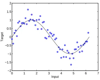
0 1 2 3 4 5 6 7 −2 −1.5 −1 −0.5 0 0.5 1 1.5 Input Target
Fig. 1.Noisy sine wave training data (dots), with noiseless generating function shown
with the solid line. Noise drawn from a Gaussian with zero mean √
.3 variance. 63
training data points (input values drawn at intervals of 0.1 from 0 to 2π).
learning this is typically confronted by the use of weight decay regularisation [2, 20] – in which a penalty term for large absolute weights is fed into the learning algorithm (the larger the weight in a sigmoidal transfer unit in an NN, the more non-linear its mapping in input space).1
Obviously this approach necessitates a prior on the weighting of this penalty. The use of EMOO approaches on the other hand allows us to optimise over all complexities. As such the problem can be cast as bi-objective for EMOO, with the first objective being the minimisation of the error function (in the regression problems shown here, the root mean square error), and the second objective being the minimisation of model complexity (here, the sum of the absolute weights of a multi-layer perceptron (MLP) neural network).
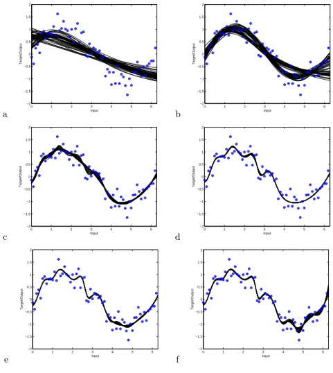
A simple example is now provided. The problem is the regression of a noisy sine wave, with the training data illustrated in Figure 1, with circles denoting the training data and the line representing the continuous (noiseless) generating process. Using a simple greedy (1+1) – evolution strategy, as described in [8, 9], one can discover the networks leading to the regressions shown in Figure 2, which correspond to points on the estimated Pareto front (dots) in Figure 3b.2 Figure 2a shows the regression lines of the 50 models with the lowest complexity
1
Other approaches have been to use pruning algorithms to remove nodes [21], other complexity loss functions [25] and topology selection methods [24].
2
For completeness an initial non-dominated set of points was generated by training a MLP (with one inputs unit, 50 hidden units and one output unit) using the quasi-newton method [2, 18] and evaluating its objectives every 50 epochs (up to 5000 epochs). The ES was run for 50000 generations, with a probability of weight mutation
(summed absolute weights) from the estimated Pareto front with Figures 2b-f showing the regression lines of groups of 50 models with consecutively higher complexity levels. a 0 1 2 3 4 5 6 −2 −1.5 −1 −0.5 0 0.5 1 1.5 2 Input Target/Output b 0 1 2 3 4 5 6 −2 −1.5 −1 −0.5 0 0.5 1 1.5 2 Input Target/Output c 0 1 2 3 4 5 6 −2 −1.5 −1 −0.5 0 0.5 1 1.5 2 Input Target/Output d 0 1 2 3 4 5 6 −2 −1.5 −1 −0.5 0 0.5 1 1.5 2 Input Target/Output e 0 1 2 3 4 5 6 −2 −1.5 −1 −0.5 0 0.5 1 1.5 2 Input Target/Output f 0 1 2 3 4 5 6 −2 −1.5 −1 −0.5 0 0.5 1 1.5 2 Input Target/Output
Fig. 2. Regression lines of the estimated Pareto optimal NNs on the training data. Plots (a)–(f) show groups of 50 models, from lowest complexity to highest complexity.
The models span the spectrum from severe under-fitting (such as the almost straight lines in Figure 2a) to severe over-fitting (such as the wiggly lines shown in Figure 2f). This range of model types is to be expected from the optimisation
of 0.1 and mutation being formed of additive draws from a zero mean Gaussian with
variance of√
0 1 2 3 4 5 6 −2 −1.5 −1 −0.5 0 0.5 1 1.5 2 Input Target/Output a 0.2 0.3 0.4 0.5 0.6 0.7 0 200 400 600 800 1000 1200 RMSE Σ w i b
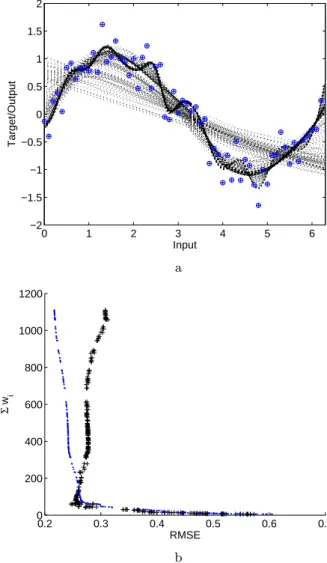
Fig. 3.a) Regression lines of the estimated Pareto optimal NNs on the training data (plotted in dotted lines). b) Estimated Pareto optimal front of NNs (dots) and the same NNs evaluated on a validation set from the same generation and noise process (crosses), note the switch back effect in the lower left corner.
a 0 1 2 3 4 5 6 7 −2 −1.5 −1 −0.5 0 0.5 1 1.5 2 Input Target/Output b 0 1 2 3 4 5 6 7 −2 −1.5 −1 −0.5 0 0.5 1 1.5 2 Input Target/Output c 0 1 2 3 4 5 6 −2 −1.5 −1 −0.5 0 0.5 1 1.5 2 Input Target/Output
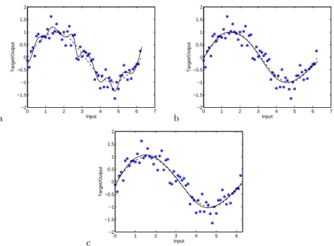
Fig. 4.a) Regression line of model with lowest RMSE on training data from estimated Pareto set. b) Regression line of model with lowest RMSE on validation data from estimated Pareto set (on training data). c) Regression line of ensemble of 10 models with lowest RMSE on validation data from estimated Pareto set (on training data).
objectives. The problem still arises as to how to choose an operating model from the set at the end of the optimisation run. One approach discussed in [10] is to evaluate the set on a second validation set of data and note at which point the complexity/accuracy curve ‘switches back’. This is shown in 3b by crosses, where a validation set of equal size as the training set is used, from the same generating process. A prominent ‘switch back’ point can be seen in the lower left hand corner, which would lead one to either choose the model with lowest root mean squared error (RMSE) in this area, or alternatively use a equal weighted ensemble of points from this region.
Figure 4 shows the regression line of various approaches with a solid line – in all cases the dashed line shows the underlying noiseless generating process. Figure 4a is the model with lowest RMSE on the training data (i.e., the model corresponding to the leftmost point in Figure 3b), Figure 4b is the model with lowest RMSE on the validation data (i.e., the model corresponding to bottom left of the ‘switch back’ cross in Figure 3b), and Figure 4c is the average regression line of the 10 models with the lowest validation error (the models at the knee of the switch back). As can clearly be seen, the model with the lowest RMSE on the training data clearly is overfitting, but the regression lines in Figures 4b and 4c
representation capability is very high (50 hidden units, with only 63 training points) the use of a complexity minimisation objective and a validation set has led to a good estimate of the noiseless generating process. Other approaches like bootstrapping or cross validation could also be employed for a similar effect. 2.2 Input selection
Input selection has been encapsulated both explicitly within supervised learning EMOO methods (as one of the objectives to be minimised (e.g. [19]), or as part of the overall complexity to be minimised (e.g. [10]). It is typically separated from model complexity measures due to the additional cost inputs can sometimes represent (the fewer inputs used, the lower the cost in sampling inputs for future classification/regression tasks). Also, the use of spurious inputs is known to impede the performance of a model [2].
2.3 Competing error terms
Another approach that has proved popular is training with multiple errors. One area of interest has been in financial applications, where there are application specific error terms (like return on investment of predicting an asset price) which when used by itself is difficult to train a model, but in conjunction with a good-ness of fit error measure can ensure that you have models that accurately predict the signaland are profitable [8, 22].
Another interesting area is the trade off between different measures of ‘good-ness of fit’. For instance, using EMOO methods one may optimise with respect to one measure (e.g. RMSE or absolute error) and also with respect to the dis-tributional properties of this principle error measure [1, 7].
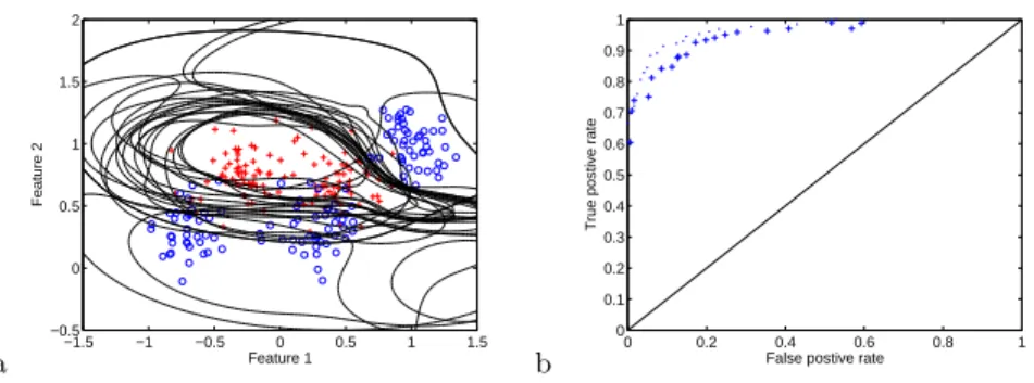
Another example of competing errors is in receiver operating characteristic (ROC) analysis, where for two class problems the true positive rate (the pro-portion of correct assignments to the principle class by the model) is traded off against the false positive rate (the proportion of incorrect assignments of the second class to the principle class by the model). The example in Figure 5a shows the decision boundaries formed by radial basis function (RBF) neu-ral network classifiers on the test problem from [12].3
Figure 5b in turn shows the estimated optimal ROC curve on the 250 training data points (shown with dots on the plot), and their evaluation on 1000 testing data points (shown with crosses on the plot). Interestingly, although not shown here (but available in [12]), synthetic ROC problems are perhaps the only supervised learning prob-lems for which the true Pareto front can be determined and the performance of the optimised solutions compared to it. This is because with a synthetic classifi-cation problem one can determine the exact posterior probability of any feature
3
The RBFs contained 10 units with Gaussian kernels, optimised in the fashion dis-cussed in [11] using a (1+1)-ES for 5000 generations with a probability of mutation
of 0.1 and variance of additive Gaussian mutation of√
a −1.5 −1 −0.5 0 0.5 1 1.5 −0.5 0 0.5 1 1.5 2 Feature 1 Feature 2 b 0 0.2 0.4 0.6 0.8 1 0 0.1 0.2 0.3 0.4 0.5 0.6 0.7 0.8 0.9 1
False postive rate
True postive rate
Fig. 5.a) Decision contours of RBF networks on estimated optimal ROC front, training data shown with one class denoted by circles and the other by crosses. b) Estimated optimal ROC front on 250 training data pairs ( denoted by dots) and their evaluation on 1000 testing data pairs (denoted by crosses).
vector, and therefore can trace out the ROC curve of Bayes rule classifier (the best possible). However, the downside to this is that when optimising a classifier based on training data from a synthetic problem, you only actually have access to an estimate of the posterior probability, not the true posterior probability (otherwise you would not need a classifier in the first place). As such the esti-mated ROC curve may actually seemin front of the known optimal curve. This problem of noise and uncertainty (which is apparent in most if not all super-vised learning problems) is one of the principle areas needing additional research in multi-objective supervised learning, and can be the source of over-optimistic assessments of performance.
3
Discussion
There are a number of other avenues in multi-objective supervised learning which have been explored using EMOO (like ensemble training, which will be the sub-ject of another workshop presentation), however the examples presented here should present a reasonable overview of the general area.
There are still a large number of open questions in the field of multi-objective supervised learning. For instance it is an area with a large number of hybrid models – usually researchers tend to either start a process with a ‘traditional’ local optimiser (like gradient descent in NNs), or iterate between a local process and an EMOO method. This tends to be because the search space is easier traversed (at least to begin with) by local methods, and because, for many of the classifiers/regressors used, the range of parameters to be searched is essentially without limits. As such EMOO techniques are often used to trace out an estimate of the Pareto front for a problem after a traditional algorithm has supplied a single point on a good estimate of the front. The question of how much search
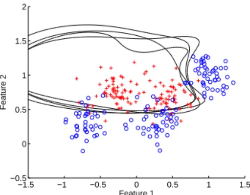
−1.5 −1 −0.5 0 0.5 1 1.5 −0.5 0 0.5 1 1.5 Feature 1 Feature 2
Fig. 6. Example decision boundaries (from RBF classifiers) with identical operating points in ROC space.
to carry out with local methods and how much time to spend searching with EMOO methods is still an open one.
To end, a few points that are worth highlighting are:
Overfitting: Unless there is an explicit casting of an objective to minimise com-plexity, EMOO approaches to optimising competing errors can be very prone to overfitting. The use of weight decay regularisation approaches in hybrid EMOOs may mitigate this somewhat – but to do this they must assume a penalty term independent of the region of objective space, which is a difficult assumption to justify.
Many to one mappings: Perhaps more than other application areas, supervised learning parameter space is full of regions which have identical evaluations in ob-jective space – especially if it is a classification problem. These disjoint plateaus can cause many problems for optimisers, and when using an elite multi-objective optimiser raises the question as to which solution to store if they have the same objective valuations but verydifferent input space partitioning. Figure 6 illus-trates this with the synthetic classification problem used earlier – the decision contours shown have identical misclassification rates on the data, but have dif-ferent decision boundaries.
Comparison: It would be interesting to see what actual benefits some of the EMOO approaches have compared to other recent methods from the Machine Learning community – for instance in feature selection tend to be compared to forwards/backwards selection, and/or another EMOO method, but recent high powered models like reversible-jump Markov chain Monte Carlo methods [3] have been largely ignored.
Noise, uncertainty, truth: Arguably the largest problem in multi-objective su-pervised learning is the fact that only samples of the generating process are available, which tend to be noisy. Optimising with uncertainty/robust optimisa-tion is an area which is gaining more interest in the general EMOO community at the current time [15, 23, 13, 14] and supervised learning problems should present an interesting avenue of research in this area.
4
A final note
The empirical examples provided have been bi-objective ones, however, this has mainly been due to ease of visualisation, and not necessarily indicative of all multi-objective supervised learning applications; for instance [4] optimises 3 ob-jectives for an air traffic alert warning system and the multi-class extension of the ROC curve developed by Everson and Fieldsend [11, 5, 6] has been applied to 6 objective problems in published work (and much higher in unpublished material).
5
Acknowledgements
The author would like to thank Michelle Fisher for helpful comments during the development of this manuscript.
References
[1] Bi, J., Bennett, K.P.: Regression Error Characteristic Curves, Proceedings of the Twentieth International Conference on Machine Learning (ICML-2003), Washington DC, pp43–50, (2003)
[2] Bishop, C.M.: Neural Networks for Pattern Recognition Oxford University Press (1999)
[3] Denison, D.G.T., Holmes, C.C., Mallick, B.K., Smith, A.F.M.: Bayesian Methods for Nonlinear Classification and Regression Wiley (2002)
[4] Everson, R.M., Fieldsend, J.E.: Multi-Objective Optimisation for Receiver oper-ating Characteristic Analysis, Yaochu Jin (Ed.) Multi-Objective Machine Learning,
Springer Series on Studies in Computational Intelligence16pp533–556 (2006)
[5] Everson, R.M., Fieldsend, J.E.: Multi-Objective Optimization of Safety Related Systems: An Application to Short Term Conflict Alert”, IEEE Transactions on
Evo-lutionary Computation,10(2), pp187-198 (2006)
[6] Everson, R.M., Fieldsend, J.E.: Multi-class ROC analysis from a multi-objective
optimisation perspective, Pattern Recognition Letters,27, pp918-927, (2006)
[7] Fieldsend, J.E.: Regression Error Characteristic Optimisation of Non-Linear Mod-els, Yaochu Jin (Ed.) Multi-Objective Machine Learning, Springer Series on Studies
in Computational Intelligence16pp103–123 (2006)
[8] Fieldsend, J.E., Singh, S.: Pareto Multi-Objective Non-Linear Regression Mod-elling to Aid CAPM Analogous Forecasting, Proceedings of the International Joint Conference on Neural Networks (IJCNN), Hawaii, May 12-17, pp388–393 (2002)
tions on Neural Networks,16(2), pp338–354 (2005)
[10] Fieldsend, J.E., Singh, S.: Optimizing forecast model complexity using multi-objective evolutionary algorithms, C.A.C Coello and G.B. Lamont (Eds) Applications of Multi-Objective Evolutionary Algorithms, World Scientific pp675–700 (2004) [11] Fieldsend J.E., Everson R.M., Formulation and comparison of multi-class ROC
surfaces Proceedings of the 2nd ROCML workshop, part of the 22nd International Conference on Machine Learning (ICML 2005) Bonn, Germany pp41–48, (2005) [12] Fieldsend, J.E., Bailey, T.C., Everson, R.M., Krzanowski, W.J., Partridge D.,
Schetinin, V., Bayesian inductively learned modules for safety critical systems Pro-ceedings of the 35th Symposium on the Interface: Computing Science and Statistics. March 12-15, Salt Lake City pp110–125, (2003)
[13] Fieldsend J.E., Everson R.M., Multi-objective Optimisation in the Presence of Uncertainty, Proceedings of the 2005 IEEE Congress on Evolutionary Computation (CEC’05) Edinburgh, UK pp476–483, (2005)
[14] Goh, C.K., Tan, K.C.: Noise Handling in Evolutionary Multi-Objective Opti-mization, Proceedings of the 2006 IEEE Congress on Evolutionary Computation (CEC’06), Vancouver, BC, Canada, July 16-21, (2006)
[15] Hughes, E.J.: Evolutionary multi-objective ranking with uncertainty and noise,
Evolutionary Multi-Criterion Optimization, EMO 2001, LNCS 1993 pp329–342,
(2001)
[16] Jin, Y., Okabe, T., Sendhoff, B.: Evolutionary multi-objective optimization ap-proach to constructing neural network ensembles for regression, C.A.C Coello and G.B. Lamont (Eds) Applications of Multi-Objective Evolutionary Algorithms, World Scientific pp653–673 (2004)
[17] Kumar, R.: On machine learning with multiobjective genetic optimization, C.A.C Coello and G.B. Lamont (Eds) Applications of Multi-Objective Evolutionary Algo-rithms, World Scientific pp393–425 (2004)
[18] Nabney, I.T.: Netlab: Algorithms for Pattern Recognition Springer-Verlag (2001) [19] Pappa, G.L., Freitas, A.A., Kaestner, C.A.A.: Multi-objective algorithms for at-tribute selection in data mining, C.A.C Coello and G.B. Lamont (Eds) Applications of Multi-Objective Evolutionary Algorithms, World Scientific pp603–626 (2004) [20] Raviv, Y., Intrator, N.: Bootstrapping with noise: An effective regularization
tech-nique, Connection Science, 8, pp356–372 (1996)
[21] LeCun, Y., Denker, J., Solla, S., Howard, R.E., Jackel, L.D.: Optimal brain dam-age, D.S. Touretzky (Ed) Advances in neural information processing systems II, pp598–605, Morgan Kaufmann (1990)
[22] Schlottmann, F., Seese, D.: Financial applications of multi-objective evolutionary algorithms: recent developments and future research directions, C.A.C Coello and G.B. Lamont (Eds) Applications of Multi-Objective Evolutionary Algorithms, World Scientific pp627–652 (2004)
[23] Teich, J.: Pareto-front exploration with uncertain objectives, Evolutionary
Multi-Criterion Optimization, EMO 2001, LNCS1993pp314–328, (2001)
[24] Utans, J., Moody, J.: Selecting neural network architectures via the prediction risk: application to corporate bond rating prediction Proceedings of the First International Conference on AI applications on Wall Street, pp35–41, IEEE Computer Society Press, (1991)
[25] Wolpert, D.: On bias plus variance, Neural Computation, 9(6), pp1211-1243,