Convolutional Autoencoder for Studying Dynamic Functional Brain Connectivity in Resting-State Functional MRI

Convolutional Autoencoder for Studying Dynamic Functional

Brain Connectivity in Resting-State Functional MRI

Fatemeh Mohammadi

A Thesis

In the Department

of

Electrical and Computer Engineering

Presented in Partial Fulfillment of the Requirements for the Degree of

Master of Science (Electrical and Computer Engineering) at

Concordia University

Montreal, Quebec, Canada

April 2019

II 2019

CONCORDIA UNIVERSITY School of Graduate Studies

This is to certify that the thesis prepared

By: Fatemeh Mohammadi

Entitled: Convolutional Autoencoder for Studying Dynamic Functional Brain Connectivity in Resting-State Functional MRI

and submitted in partial fulfillment of the requirements for the degree of

Master of Applied Science(Electrical and Computer Engineering)

Complies with the regulations of the University and meets the accepted standards with respect to originality and quality.

Signed by the final examining committee:

Chair Dr. External Examiner Dr. Examiner Dr. Supervisor Dr. M. O. Ahmad Supervisor Dr. M.N.S. Swamy Approved by Dr. W. E. Lynch, Chair Department of

Electrical and Computer Engineering

Dr. Amir Asif, Dean

III

ABSTRACT

Convolutional Autoencoder for Studying Dynamic Functional Brain Connectivity

in Resting-State Functional MRI

Fatemeh Mohammadi

Brain is the most complex organ in human body. Understanding how different regions of the brain function and interact with one another is a challenging task. One of the most important topics in the study of the brain is the functional brain connectivity, which is defined as the correlations, each between a pair of the activation signals from the different regions of the brain. Study of the functional connectivity in the human brain provides new insights into the understanding of the healthy and diseased brains and their differences. Functional magnetic resonance imaging (fMRI) is an imaging technique that allows researchers to study the brain activity and functional connectivity. While many researchers have focused on static functional connectivity in the resting-state fMRI to study the functions of the brain, dynamic functional connectivity has received more attention recently for such a study, since it provides more detailed information about the brain functions. Within the literature for studying the dynamic brain connectivity, k-means clustering has been applied to the connectivity matrices in order to find the functional connectivity patterns. However, it is known that the k-means clustering technique is not suitable for applying it to high dimensional data such as the functional brain connectivity matrices. In this thesis, in order to overcome this problem, we propose a deep learning-based convolutional autoencoder to obtain

IV

latent representations of the connectivity matrices prior to applying to them the k-means clustering. Use of the convolutional autoencoder, not only reduces the dimension of the connectivity matrices, but also provides a more semantic representation of these matrices. It is shown that the proposed method of clustering that consists of the use of the autoencoder followed by k-means clustering results in improving the clustering of the connectivity matrices, and consequently, to a better capturing of the functional connectivity patterns. In order to show the effectiveness of the proposed clustering method, synthetic connectivity matrices for patterns, with their classes known, are generated. The proposed method is then first applied to these syntactically generated connectivity matrices and the resulting patterns are compared with that obtained by applying k-means clustering technique to the synthetic connectivity matrices. It is shown that the proposed method classifies the various patterns more accurately.

The proposed method is then used to study the dynamic functional brain connectivity by applying it to real fMRI data captured from a group of healthy subjects and another group of subjects affected by schizophrenia. For this purpose, after preprocessing the raw fMRI data for each subject in these two groups, the group independent component analysis (ICA) is applied in order to decompose the fMRI data into statistically independent components (map of the entire brain) and their corresponding time-courses. Each independent component corresponds to a specific region of the brain. The connectivity matrix whose elements corresponds to the correlation between the time-courses within a segment of the time-courses enclosed inside a sliding window is then obtained. Next, the proposed clustering method is used to cluster all the connectivity matrices, each corresponding to one segment, into a finite number of functional connectivity patterns (states). A two-sample t-test is then performed on each state in order to determine each pair of the regions in the group of the healthy control subjects for which weather or not the correlation value

V

is significantly different from that of the corresponding pair of the regions in the group of schizophrenia patients. It is observed through this test that there are indeed pairs of the brain regions where significant differences do exist between the two groups. It is also seen that such a difference between the two groups is even more pronounced in the visual network of the brain.

Finally, in this thesis, a study is undertaken for the evaluation of the dwell time, which is defined to be the duration for a functional connectivity pattern to remain in one state before switching to another state. It is shown through this study that the dwell time for the healthy group to stay in the state with more connectivity is longer than that for the group with schizophrenia. On the other hand, the dwell time for the group with schizophrenia to stay in the state with less connectivity is longer than that for the healthy group.

VI

ACKNOWLEDGEMENTS

It is my pleasure to express my deep gratitude and thanks to my supervisors, Professor M.O. Ahmad and Professor M.N.S Swamy for their continuous guidance and support throughout the course of this research. Their valuable suggestions have been very useful and were among the major reasons that enabled me to pursue my research. It has been an honor and privilege to work under their supervision. I would never forget their support and affection throughout my research period, and I am deeply grateful for them.

Special thanks and gratitude are due to my beloved husband, Yaser, for his patience, encouragement and support. I am so thankful to have him in my life. I would like also to thank my parents and friends who supported me and were available in times of need and eased the hardships of my life. Special gratitude to my mother and my father who are the first inspiration for me in the field of research work.

VII

TABLE OF CONTENTS

LIST OF FIGURES ... X LIST OF TABLES ... XIV LIST OF SYMBOLS ... XV LIST OF ABBRIVIATIONS ... XVII

CHAPTER 1: Introduction ...1

1.1 Background ... 1

1.2 Human Brain ... 1

1.3 Functional and Anatomical Brain Connectivity ... 2

1.4 Functional MRI ... 3

1.5 Resting-State fMRI ... 5

1.6 Resting-State Networks ... 7

1.7 Static and Dynamic Functional Connectivity ... 7

1.8 Functional Connectivity Analysis ... 8

1.9 Brief Literature Review Survey ... 9

1.10 Motivation and Thesis Objective ... 10

1.11 Organization of the Thesis ... 11

CHAPTER 2: Background Material ...13

2.1 Introduction ... 13

2.2 Preprocessing of fMRI Images ... 13

2.2.1 Slice Timing Correction ... 13

VIII

2.2.3 Coregistration ... 15

2.2.4 Normalization ... 16

2.2.5 Spatial Smoothing ... 16

2.3 Independent Component Analysis ... 17

2.4 ICA in fMRI ... 19

2.5 Group ICA ... 21

2.6 Component Selection ... 23

2.7 Dynamic Functional Brain Connectivity ... 25

2.8 K-means Technique ... 27

2.9 Two-Sample T-Test ... 29

2.10 Summary ... 30

CHAPTER 3: Group Difference Study Using Convolutional Autoencoder...31

3.1 Introduction ... 31

3.2 Introduction to Neural Networks ... 32

3.3 Convolutional Neural Networks ... 35

3.3.1 Convolutional Layer ... 36

3.3.2 Pooling Layer ... 38

3.4 Convolutional Autoencoder ... 39

3.5 The Pipeline of Dynamic Functional Brain Connectivity Study ... 41

3.5.1 Group ICA and Windowing ... 41

3.5.2 Convolutional Autoencoder for Obtaining FC States ... 41

IX

3.6 Summary ... 43

CHAPTER 4: Results and Discussions ...45

4.1 Introduction ...45

4.2 What Is Schizophrenia? ... 46

4.3 fMRI Data Analysis ... 46

4.4 Analysis of Group Differences ... 62

4.5 Summary ... 68

CHAPTER 5: Conclusion and Future Work ...70

5.1 Conclusion ... 70

5.2 Future Work ... 72

X

List of Figures

Figure 1.1: a) The structure of a typical neuron in human brain [3]. b) A vertical cut of brain showing grey matter and

white matter tissues [4] ...2

Figure 1.2: a) White matter fiber tracking using DTI. b) Functional connectivity map showing the coactivation between some brain regions [7]………...3

Figure 1.3: Increasement in blood flow resulted from brain neural activity leads to increasing glucose and oxygen and decreasing in deoxyhemoglobin [17] ………...4

Figure 1.4: fMRI data as a time sequence of 3D images [18].………..…....5

Figure 1.5: An fMRI scanner; a functional magnetic resonance imaging equipment using a strong magnetic field to measure brain activity [24]……….6

Figure 1.6: Common resting-state networks [25] ……….7

Figure 2.1: Time slicing, a preprocessing step for fMRI data [42,43]...14

Figure 2.2: Realignment of slices ...15

Figure 2.3: Coregistration, aligning the functional MRI data with structural image ...15

Figure 2.4: MNI space, averaged anatomical images of 152 subjects[45] ...16

Figure 2.5: Separating mixed speech data recorded by microphones using ICA [47] ...17

XI

Figure 2.7: Decomposition of fMRI images using ICA. Each row of 𝑋 is a scan of brain flattened at a certain time point; Each column of 𝐴 is a coefficient (time course) of the corresponding component; Each

row of 𝑆 is an independent component [50] ...20

Figure 2.8: Applying ICA to the concatenated dimension reduced data of different subjects ...21

Figure 2.9: An example of the brain functional connectivity matrix. The independent brain components are separated into seven groups. Sub-cortical (SC), auditory (AUD), visual (VIS), sensorimotor (SM), cognitive control (CC), default mode (DM) and cerebellar (CB) ...25

Figure 2.10: Obtaining the functional connectivity matrices by using a sliding window [52] ...27

Figure 2.11: K-means clustering fails to put image (b), (c) and (d) in the same cluster as image (a) [54] ...28

Figure 2.12: Two independent populations [55] ...29

Figure 3.1: The pipeline of dynamic functional brain connectivity study ...31

Figure 3.2: The physiological representation of a neuron [57] ...32

Figure 3.3: The computation in a neuron ...33

Figure 3.4: The most common activation functions [59] ...33

Figure 3.5: A typical structure of a multi-layer neural network……….35

Figure 3.6: A typical architecture of a convolutional neural network [60]…………36

XII

Figure 3.8: Max pooling operation [63]……….38 Figure 3.9: The general architecture of a convolutional autoencoder [64]…………....40 Figure 4.1: An independent component (IC) and the corresponding time-course…...50 Figure 4.2: The output of GIFT software showing an independent component,

its corresponding time-course and frequency spectra……….51 Figure 4.3: The output of GIFT software showing an independent component,

its corresponding time-course and frequency spectra……….52 Figure 4.4: The architecture of the designed convolutional autoencoder for

obtaining functional connectivity patterns…………...….………...54 Figure 4.5: Loss curve for the convolutional autoencoder during the training…...54 Figure 4.6: One sample of synthetic connectivity matrices from each pattern.……...56 Figure 4.7: Visualization of the synthetic connectivity matrices using t-SNE…………57 Figure 4.8: T-SNE visualization of the latent representations of the

generated connectivity matrices obtained by the designed CAE ….………58 Figure 4.9: Average of the correlation matrices in each state. …………..……….…….60 Figure 4.10: Median of correlation matrices in each state for the healthy

control subjects …..………...……….…….………61 Figure 4.11: Median of correlation matrices in each state for the

schizophrenia patients. ………62 Figure 4.12: Two-sample t-test results showing FC differences between pairs of the brain regions in the healthy control (HC) subjects and corresponding brain regions in the schizophrenia (SCZ) subjects in each state

XIII

Figure 4.13: The regions in the visual network part of the brain where significant

differences exist between those in groups of HC and SCZ ………...65 Figure 4.14. Two-sample t-test results showing FC differences between

pairs of the brain regions in the healthy control (HC) subjects and corresponding brain regions in the schizophrenia (SCZ) subjects in each state obtained by using the traditional clustering method

of k-means.. ……….………...66 Figure 4.15: Average dwell time in each state for the HC and SCZ group………....67 Figure 4.16: Average dwell time in each state for the HC and SCZ groups after

XIV

List of Tables

Table 4.1: Summary of subject demographic ...46 Table 4.2: Convolutional autoencoder layers ...55 Table 4.3: Number of matrices in different clusters ...59

XV

List of Symbols

𝐴 Mixing matrix

𝐴𝑖 Coefficient corresponding to the component 𝑆𝑖

𝐶 Inverse of the matrix 𝐴 𝐷 Number of sliding windows

𝐹_𝑖 Reducing matrix determined by PCA (Subject-level)

𝑓 Filter size (Kernel size)

𝐺𝑖 Reducing matrix determined by PCA (Group-level)

𝐾 Number of clusters

𝐿 Number of rows in a dimension-reduced fMRI data

𝑀 Number of subjects

𝑁 Number of independent components

𝑆 Matrix of independent components

𝑂 Output of a neural network

𝑝 Padding size

𝑞 Stride size

𝑆_𝑖 𝑖𝑡ℎ _{independent component}

𝑇 Number of signals (Number of fMRI scans)

𝑉 Length of each signal

𝑊 Length of the sliding window

XVI

𝑋 Matrix of data

𝑌 Dimension-reduced fMRI data of a subject

𝛼

∅

XVII

List of Abbreviations

ANN Artificial Neural Network AU Auditory

BOLD Blood Oxygen Level Dependent CAE Convolutional Autoencoder CB Cerebellum

CC Cognitive Control

CNN Convolutional Neural Network CSF Cerebrospinal Fluid

DMN Default Mode Network EEG Electroencephalography FC Functional Connectivity

FMRI Functional Magnetic Resonance Imaging FOV Field of View

ICA Independent Component Analysis MEG Magnetoencephalography

MNI Montreal Neurological Institute MRI Magnetic Resonance Imaging PCA Principal Component Analysis RELU Rectified Linear Unit

ROI Region of Interest RSN Resting State Network

XVIII SC Subcortical

SPM Statistical Parametric Mapping SM Sensorimotor

T-SNE T-Distributed Stochastic Neighbor Embedding TR Time to Repetition

VIS Visual WM White Matter

1

CHAPTER 1

:

Introduction

1.1 Background

Functional MRI (fMRI) has the potential to open novel insights to the understanding of the brain functions. It is considered to be a noninvasive and safe technique for visualizing and mapping functional brain activity. Functional MRI is also used to investigate the connectivity patterns among the different brain regions. This functional connectivity study can be carried out using fMRI in resting-state or during task-related experiments. In this thesis, we focus on the functional connectivity in resting-state fMRI. Functional connectivity (FC), which is the correlation between activation signals of different brain regions, has been assumed for a long time to have a stationary nature. It has been only recently that the dynamic behavior of FC is revealed, showing the functional connectivity between different brain regions have meaningful variations in resting-state fMRI [1]. Therefore, some works have been done to assess and characterize the dynamic FC (dFC) in order to explore how the brain functions in healthy people and in people with different psychological disorders.

In order to study the functional connectivity using fMRI data, it is necessary to understand the basis of the brain structure and the functional imaging tool.

1.2 Human Brain

Brain is the most complex organ inside human body that has billions of nerves communicating through passing electrical signals at junctions called synapses. Anatomically, brain tissue consists of grey matter (GM) and white matter (WM). The grey matter that includes neuron cell bodies and dendrites is responsible for the most of high-level brain functional processes. The white matter

2

(a) (b)

that consists of bundles of long myelinated axons is responsible for transferring of the information to different grey matter regions. There is also a clear liquid in the brain and spinal cord called cerebrospinal fluid (CSF) [2]. Figure 1.1. (a) and Figure 1.1. (b) demonstrate a typical neuron in human brain and a vertical cut of the brain, respectively.

1.3 Functional and Anatomical Brain Connectivity

Our brain is a network of many different brain regions. Each brain region is specialized in performing specific tasks and functions. Structural connections in the brain mainly refer to anatomical pathways that directly interconnect spatially separated brain regions. Diffusion tensor imaging (DTI) is an imaging technique for visualizing anatomical connections [5] as shown in Figure 1.2. (a). On the other hand, the functional connectivity is defined as the pattern of temporal correlation made by the interactions between segregated brain region pairs [6]. In other words,

Figure 1.1. a) The structure of a typical neuron in human brain [3]. b) A vertical cut of brain showing grey matter and white matter tissues [4].

3

functional connectivity shows the statistical relationship between the signals of different brain regions. Study of the functional connectivity among brain regions can be done by using the functional magnetic resonance imaging (fMRI). Figure 1.2. (b) illustrates an example of functional map showing the relationship between the activity of brain regions.

1.4 Functional MRI

Functional magnetic resonance imaging (fMRI) is an imaging tool providing a high spatial resolution, noninvasive and safe technique for visualizing and mapping the functional brain activity. It is used in a growing number of studies [8-11] to understand the functionality of a human brain and to explore interaction, connection and coordination of different parts of the brain. It is also used to study the differences in the brain functionality of healthy people and people affected by some psychiatric brain disorders [12-14].

(a) (b)

Figure 1.2. a) White matter fiber tracking using DTI. b) Functional connectivity map showing the coactivation between some brain regions [7].

4

Figure 1.3. Increasement in blood flow resulted from brain neural activity leads to increasing glucose and oxygen and decreasing in deoxyhemoglobin [17].

The basis of the fMRI sensitivity to the brain neural activity arises from the local magnetic field changes. Oxygenated and deoxygenated blood have different paramagnetic properties. In contrast to deoxygenated blood that is paramagnetic, oxygenated blood is diamagnetic i.e. it causes almost no effect on the magnetic field. Upon neural activation of a local brain area, blood flow increases in order to provide more oxygen and glucose to that area. Consequently, the blood deoxyhemoglobin concentration decreases, as shown in Figure 1.3. This causes a distortion in the magnetic field and an increase in the blood-oxygen-level dependent (BOLD) signal. In fMRI, the contrast in the BOLD signal is used to observe the different areas of the brain, activated at a given time [15, 16].

Compared with other methods, such as EEG and MEG, fMRI provides a higher spatial resolution and thus has got a lot of interest from researchers [8-11]. In fMRI, scans of the whole brain are acquired over time. Each scan includes slices of the brain volume. The time resolution (TR) is defined as the time between two sequential scans of the same point in the brain. The temporal resolution (TR) is usually 2–3 seconds. Each scan of fMRI is a three-dimensional image (a 3D volume) and the term voxel is referred to an element of this 3D volume. The value of each voxel

5

Figure 1.4. fMRI data as a time sequence of 3D images [18].

changes from one scan to another scan over time. Hence, as shown in Figure 1.4, fMRI is a 4D data where three dimensions are used to reconstruct voxels in the space and fourth dimension (time) measures the activation of each voxel over time.

1.5 Resting-State fMRI

Brain consumes 20% of the energy in the body during spontaneous brain activity. Only a small percentage of the energy consumed by the brain is used for task-related activities [19]. In view of this, study of the resting-state fMRI is shown to be important. In the resting-state fMRI, a subject who lies inside the fMRI scanner is trained to let his mind wonder without doing any specific task. In contrast, there is another type of study for task-related fMRI that tries to find spatial activation pattern of human brain when a subject performs a cognitive task. Figure 1.5 illustrates an fMRI scanner where a subject lies inside it.

6

Biswal et al. [20] were the first researchers who found out that the left and right hemispheric regions of the primary motor network show a high synchronization between their BOLD time courses during resting-state experiment. Since then, researchers have been able to map the intrinsic functional connection diagram of brain without using any designed tasks and resting-state studies have received lots of attention [21, 22]. Also, the resting-state fMRI allows researchers to study the brain function of patients who are not able to do complicated tasks or long experiments. In contrast to the task-based functional imaging that typically highlights a single brain region associated to any given task, the resting-state fMRI highlights the activity among different brain regions at once. Hence, study of the resting-state fMRI is valuable for varieties of research topics including the study of psychological brain disorders [14]. The resting-state fMRI can also be used to study and compare the functional activities in the different brain regions of two different groups, such as patients with Schizophrenia and healthy subjects [23].

Figure 1.5. A fMRI scanner; a functional magnetic resonance imaging equipment with a strong magnetic field to measure brain activity [24].

7

Figure 1.6. Common resting-state networks [25].

1.6 Resting-State Networks

It has been shown in the resting-state functional studies that there are some groups of brain regions in which a strong functional connectivity exists. In other words, these regions activate and deactivate together during rest. These brain regions are the same across all subjects and are referred to as resting-state networks (RSNs) [21, 22]. Default Mode, Visual, Auditory, Cognitive Control/Attention, Sensorimotor and Cerebellum are some of the most common RSNs in different studies, their locations in the brain are shown in Figure 1.6.

1.7 Static and Dynamic Functional Connectivity

Study of the functional connectivity (FC) can be carried out by considering FC to be static or dynamic. Static functional connectivity is obtained by finding the correlation between activation signals of different brain regions over the course of many minutes, assuming the FC does not

8

change in time. Although the static functional connectivity provides useful information, many years of research has shown that the brain activity is not constant and varies in time [26-28]. In view of this, finding the correlation between the activation signals of different brain region pairs across 5-10 minutes of fMRI recording results in losing a lot of information about their functional connectivity. Hence, the functional connectivity should be measured within time in a dynamic way. The dynamic functional connectivity is measured by obtaining the time-varying correlation between activation signals of different brain region pairs within fMRI recording time. There are different methods for analyzing fMRI functional connectivity. Generally, these methods are grouped into two types: model-based methods and data-driven methods [29].

1.8 Functional Connectivity Analysis

In many studies [30-32], the analyses of the functional brain connectivity are carried out by using the model-based approaches. In the model-based analysis, the connection between the regions of interest (ROI) is calculated by using some matrices, such as cross-correlation to generate the functional connectivity map of the human brain. Selecting the regions of interest needs some prior knowledge about the anatomy of brain. By using the model-based analysis, we need to make decisions on the size, shape and location of the regions of interest that may lead to the different outcomes in the functional connectivity analysis.

On the other hand, there are some data-driven approaches that are based on the features extracted from the input data (fMRI data). The advantage of using these approaches is that they do not require a prior selection of the brain regions and are able to decompose the captured fMRI data into a set of separated brain regions. It is helpful to evaluate the functional connectivity in fMRI data without considering any prior information about its spatial or temporal pattern. The most

9

commonly used methods to achieve such a decomposition are independent component analysis (ICA) and principle component analysis (PCA) [21,29].

1.9 Brief Literature Review Survey

Assessment of the functional connectivity using the resting-state fMRI underlines specific information across the whole brain. The recent studies have shown that the functional brain connectivity in the healthy people is different from that in the people affected by mental diseases [11,12,13,22]. For many years, researchers have studied the static functional connectivity assuming the temporal dependency among different brain regions is global and constant during a few minutes of resting-state fMRI recording [33, 34]. However, other studies using high temporal resolution techniques such as electroencephalogram (EEG) and magnetoencephalography (MEG) have shown the problem with this assumption and have observed that there are spontaneous changes in the brain activity [35, 36]. Hence, the assumption of the functional connectivity being static and constant during a resting-state fMRI experiment is an over-simplification despite its convenience. Given the increasing evidence on the importance of dynamic functional connectivity in the resting-state fMRI for assessing intrinsic function of the brain, the researchers’ focus has shifted from static functional connectivity to time-varying or dynamic functional connectivity. The study by Allen et al. in 2013 [8] is one of the first major works on time-varying functional connectivity, usually referred to as dynamic connectivity, using resting-state fMRI. In this study, the assessment of the whole-brain dynamic functional connectivity was investigated employing three major steps. First, a data driven technique (spatial independent component analysis) is applied to the fMRI data to decompose it into independent components and the corresponding time courses. In the second step, by passing a sliding window through time-courses, correlation matrices that show the degree to which each region is correlated with other regions of brain are obtained.

10

Finally, the correlation matrices are clustered for the purpose of studying the dynamic properties of functional brain connectivity. There are some other studies based on the pipeline proposed in [8] to investigate the dynamic functional connectivity in different brain diseases including the work done by Yao et al. [38,39] and [40] for studying the time-varying functional connectivity in autism and bipolar disorder, respectively. The limitation of the proposed procedure in [8] for finding the dynamic functional connectivity is that the clustering of the correlation matrices for capturing different dynamic functional connectivity patterns has been carried out by k-means method. However, the k-means method has been shown to be suboptimal for being applied to the high dimensional data. In 2015, Yaesoubi et al. [37] proposed a novel pipeline to characterize the functional interactions among the different brain regions using time-frequency analysis. One advantage of the pipeline proposed in [37] over the one in [8] is that there is no need to exploit the sliding windows to capture the dynamic functional connectivity. However, the problem with the proposed method in [37] is that the interpretability of the functional connectivity results is so difficult in time-frequency domain. Hence, the pipeline proposed in [8] is more dominant in neuroscience community for studying the dynamic functional connectivity in the healthy and diseased brains using the resting-state fMRI. It should be noted that the proposed method in [37] also has the same limitation as [8] that is the use of k-means for clustering the different functional connectivity patterns.

1.10 Motivation and Thesis Objective

As mentioned in previous section, applying the k-means clustering to the functional connectivity matrices for finding the reoccurring functional connectivity patterns is one of the common steps in most of the works [8, 37, 38, 40]. In general, the k-means clustering is a suitable option for the

11

clustering of low dimensional data. However, this method does not perform well for high dimension data such as images. It is resulted from the fact that using Euclidian distance over high dimensional spaces (such as images with lots of pixels) is not intuitive. An example of high dimensional data is the 28×28 images of MNIST handwritten digits in which the k-means has been shown to fail in clustering them properly [41]. In view of this, we concluded that applying the k-means method to the correlation matrices for finding the connectivity patterns (as done in most of the other works) is not optimal and can lead to an inaccurate result. In this thesis, as the main contribution we address this issue by using a convolutional autoencoder for obtaining the correlation matrices with the common functional connectivity patterns. By using these connectivity patterns, we can study the differences between the functional brain connectivity in the healthy control subjects and that in patients.

1.11 Organization of the Thesis

This thesis is organized as follows. In Chapter 2, the background materials used in this thesis for studying the functional brain connectivity are presented. This chapter is divided into three main parts. In the first part, the preprocessing steps that are typically applied to the raw fMRI data for reducing the artifact and noise are explained. In the second part, the theoretical background about the independent component analysis and its extension, called group ICA are presented. Then, we explain about applying the group ICA to the fMRI images and obtaining the correlation matrix from pairwise correlation between time-courses corresponding to independent components. In the last part of Chapter 2, we explain the process of obtaining the dynamic functional brain connectivity using sliding windows. In Chapter 3, the whole procedure for obtaining the dynamic functional connectivity in this study is presented. The Chapter 3 is divided into two main parts. In

12

the first part, the neural networks and convolutional autoencoders for extracting latent representations are explained. In the second part of the chapter, for the first time, we propose using the convolutional autoencoders for obtaining the dynamic functional brain connectivity patterns. In Chapter 4, the procedure developed in Chapter 3 is applied to the data gathered from 72 healthy control subjects and 74 patients affected by schizophrenia. After following the procedure given in Chapter 3, including the preprocessing, group ICA and using the convolutional autoencoder for clustering the connectivity matrices, a two-sample t-test is performed on each cluster in order to determine each pair of the brain regions in the group of the healthy control subjects for which the correlation value is significantly different from that of the corresponding pair of in the group of patients.

13

CHAPTER 2: Background Material

2.1 Introduction

In this chapter, the background materials that are directly linked to study of the functional brain connectivity are presented. First, the preprocessing steps for fMRI data is explained in detail in Section 2.2. In Section 2.3 and 2.4, the concept of independent component analysis (ICA), its statistical characteristics and its usage for the extraction of fMRI components are described. Next, in Section 2.5 group ICA method for overcoming the limitation of ICA in the group study of fMRI data are explained. Selecting the suitable ICA components (output of group ICA) and excluding the artifact components is then discussed in Section 2.6. In Section 2.7, the framework for obtaining the dynamic functional brain connectivity is presented. Finally, the two-sample t-test method for finding the group differences is described.

2.2 Preprocessing of fMRI Images

In order to reduce the artifact and noise in the fMRI data, preprocessing procedures are commonly applied to raw functional MRI data prior to applying any other statistical method. The common preprocessing steps, including slice timing correction, realignment, coregistration, normalization and spatial smoothing are explained in detail in the following subsections.

2.2.1 Slice Timing Correction

In fMRI, scans of the whole brain are acquired over time. Each scan itself includes slices of the brain volume. These slices are not acquired at the same time. For example, for a scan of 30 slices and a TR of 3 seconds, the last slice is taken 3 seconds after the first slice. Since for analyzing the

14

fMRI data, the assumption is that all the slices of each scan are acquired at once, slice timing correction preprocessing step is exploited to overcome the problem of time differences among the slices in a scan. In more detail, in this preprocessing step, one of the slices of each scan (commonly the middle slice) would be considered as the reference slice, all the other slices of its corresponding scan would be shifted in time according to the reference slice as shown in Figure 2.1. Hence, after applying time-slicing correction to the fMRI data, all the slices in each scan can be considered to be acquired at the same time.

Figure 2.1 Time slicing, a preprocessing step for fMRI data [42, 43].

2.2.2 Realignment

Another preprocessing step applied to the fMRI data is realignment. During the recording of the fMRI data, subjects might move their head slightly. It can result in adding noise to the fMRI data and consequently making the analysis of fMRI data difficult. During analysis of fMRI data, we have to make sure that a time course represents values from the same voxel location in each fMRI scan. Hence, the head movement problem should be addressed by applying the realignment procedure to the fMRI data prior to starting the fMRI analysis. In the realignment procedure, the difference between consecutive slices of fMRI images are minimized and the slices are aligned by using 6 parameters (3 translations in X, Y and Z directions and 3 rotations around the X, Y and Z

15

Figure 2.2 Realignment of slices.

Figure 2.3Coregistration, aligning the functional MRI data with structural image.

axes), so that all the slices would have the same orientation. Figure 2.2 shows the realignment of the slices in a scan of the fMRI data.

2.2.3 Coregistration

Coregistration is another important step in the preprocessing of fMRI data. Coregistration refers to the alignment of the functional images to the structural image from the same subject brain by maximizing the mutual information. An example of the coregistered anatomical and functional fMRI data are shown in Figure 2.3. As the result, the coregisteration is useful for visualizing the brain activation on a higher spatial resolution image of the brain.

16

Figure 2.4MNI space, averaged anatomical images of 152 subjects [45]. 2.2.4 Normalization

Normalization is an important preprocessing step that is applied to the fMRI data after coregistration. Since people have different shape of brain, the normalization step is required for aligning the fMRI data of different subjects to a standard template such as the one shown in Figure 2.4 that is Montreal Neurological Institute (MNI) space. The MNI template is obtained from taking the average of brain anatomical images of 152 subjects. After transforming the fMRI data of all subjects into the same space, the location of a voxel remains the same across all the subjects. Hence, after applying the normalization, we are able to compare the fMRI data across subjects.

2.2.5 Spatial Smoothing

The last preprocessing step for fMRI data is spatial smoothing. In the spatial smoothing step, the main goal is to remove the high frequency noise and artifact from fMRI data. For this purpose, a gaussian kernel is spatially convolved to the fMRI images in order to increase the signal to noise ratio. After convolving a gaussian kernel with the image, the value at each voxel will be replaced by a weighted average of the values in surrounding voxels.

17

Figure 2.5. Separating mixed speech data recorded by microphones using ICA [47].

(2.1)

After applying the above-mentioned preprocessing procedures to the fMRI data, the resulting fMRI data are prepared for further analysis, such as applying ICA.

2.3 Independent Component Analysis

Independent component analysis (ICA) is a statistical method used to extract unknown source signals from their linear mixtures based on an assumption that the source signals are statistically independent and non-gaussian [46]. In other words, ICA tries to decompose a data into a linear combination of the independent source signals (independent components) without having any prior information about these source signals. A classic example of ICA is shown in Figure 2.5.

If our data consist of 𝑇 signals, each with length 𝑉, we can arrange them into a matrix 𝑋𝑇×𝑉 with

𝑇 rows and 𝑉 columns. Then, by applying ICA, the data decomposes to 𝑁 independent component as shown bellow

𝑋 = 𝐴𝑆 = ∑ 𝐴𝑖𝑆𝑖 𝑁

18

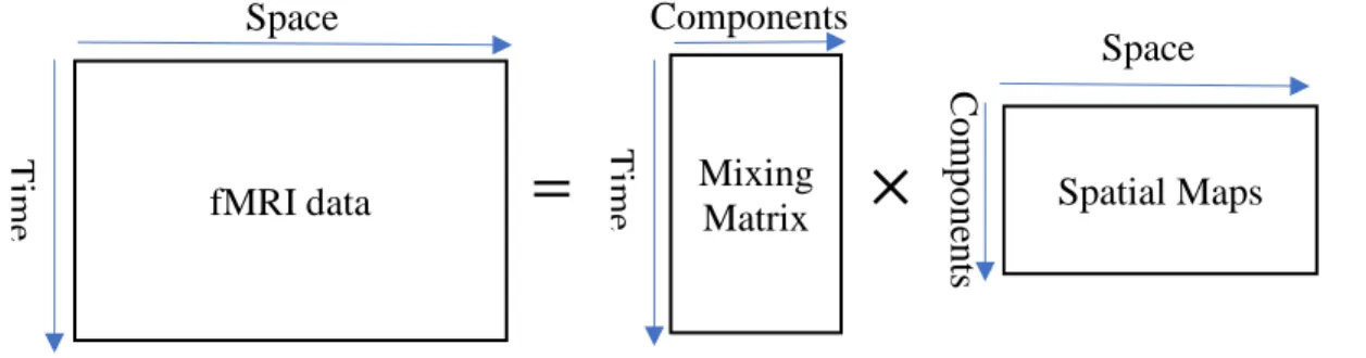
Figure 2.6. Applying ICA to fMRI data. fMRI data Space Components Time Time Spatial Maps C omponents Space (2.2)

where 𝑆 is a N × V matrix, 𝑆𝑖 is the 𝑖𝑡ℎrow of matrix S (𝑖𝑡ℎ independent component) and A is a T × N mixing matrix. The 𝑖𝑡ℎ column of 𝐴, 𝐴𝑖, represents the coefficients corresponding to the component 𝑆𝑖. It should be noted that we only observe the data 𝑋, and both 𝐴 and 𝑆 need to be estimated.

= ×

The matrix 𝑆 can be obtained by multiplication of matrix 𝑋 by matrix 𝑊 as

𝑆 = 𝐶𝑋

where 𝐶 is the inverse of the matrix 𝐴. Hence, a linear combination of the 𝑥_𝑖, 𝑥_𝑖 is the 𝑖𝑡ℎ column of 𝑋, can estimate one of the independent components. In other words, if 𝑐 be one of rows of 𝐶,

𝑦 = 𝑐𝑇𝑥 is a linear combination that result in one of the independent components. According to the central limit theorem the distribution of sum of independent random variables is closer to gaussian distribution than the distribution of the original variables. In order to estimate 𝑐, we first consider a change of parameter as 𝑧 = 𝐴𝑇𝑐 so that 𝑦 = 𝑐𝑇𝑥= 𝑐𝑇𝐴𝑠 = 𝑧𝑇𝑠. Based on the central limit theorem, 𝑧𝑇_{𝑠 is more gaussian than any of the 𝑠}

𝑖 and the gaussianity of 𝑧𝑇𝑠 is minimized when it equals to one of the independent components (𝑠_𝑖). In other words, taking 𝑐 to maximize the nongaussianity of 𝑐𝑇𝑥 = 𝑧𝑇𝑠 is equivalent to have the vector 𝑧 with only one non-zero element. In this case, 𝑐𝑇_{𝑥 gives one of the independent components [45]. Quantitative measures of the} non-gaussianity for ICA estimation are using kurtosis, negentropy and approximation of negentropy.

Mixing Matrix

19

For example, in FastICA, a popular algorithm for estimation of independent components, non-gaussianity is maximized by using the approximation of negentropy which is faster and more robust than kurtosis. Another approach for estimation of independent components in ICA is minimization of mutual information that is shown to be equivalent to maximizing the nongusianity. In the Infomax ICA algorithm that is one of the most popular ICA algorithms, the independent components are estimated by minimizing the mutual information.

2.4 ICA in fMRI

Since in the resting state fMRI we have no prior information in time and in location, there is an increasing interest in applying ICA algorithm to the resting-state fMRI data for studying the spatial and temporal properties of fMRI data [8, 21, 23, 25, 26, 38, 48]. ICA works based on an assumption that BOLD fMRI time series are generated by linear mixture of neural activities.

There are two approaches for applying ICA to achieve maximal independence components in space or in time for analyzing fMRI data. 1- Spatial ICA, which extracts independent spatial images and a set of corresponding time courses, 2- temporal ICA, which extracts independent time courses and a corresponding set of images [49]. Analysis of spatially independent components is by far the most common approach in fMRI studies. In our work, the application of ICA is to determine spatially separate brain regions and their corresponding time courses with aim to studying functional brain connectivity. Therefore, spatial ICA, is more appropriate for the task of this research. A schematic representation of the spatial ICA applied to the fMRI data is shown in Figure 2.7.

As explained in chapter 1, fMRI data is a 3D data (scan) at any given time. In order to prepare our data, we can flatten each of these scans and put it into a row of a matrix, 𝑋. Hence, each row in

20

Figure 2.7. Decomposition of fMRI images using ICA. Each row of 𝑿 is a scan of brain flattened at a certain time point; Each column of 𝑨 is a coefficient (time course) of the corresponding component; Each row of 𝑺 is an independent component [50].

Time 1

matrix 𝑋 represents all the voxels of a fMRI scan at a fixed time point and each column represents a single voxel time series. The matrix 𝑋 is a 𝑇 by 𝑉 matrix, where 𝑇 and 𝑉 are the number of time points and the number of voxels in a fMRI scan, respectively. ICA decomposes the matrix X (the original fMRI data) into an independent component matrix S and its respective mixing matrix 𝐴

as shown in Figure 2.7 by maximizing the statistical independence of the estimated components through an iterative optimization procedure.

𝑆 is a N × V matrix (𝑁 is the number of components and 𝑉 is the number of voxels in each scan) and 𝑆_𝑖is the 𝑖𝑡ℎindependent component of fMRI data. Matrix 𝐴is a T × N mixing matrix and each column of 𝐴 with length 𝑇 is called the time course corresponding to 𝑖𝑡ℎ IC in matrix S (𝑠_𝑖). Therefore, there is a time course corresponding to each independent component. The statistical relationship between each pair of the time-courses specifies the functional connectivity between the corresponding pair of the components.

21

Figure 2.8 Applying ICA to the concatenated dimension reduced data of different subjects.

2.5 Group ICA

ICA is suitable to be applied to a single subject fMRI data. However, the problem with using ICA in fMRI data comes from the arbitrary order of the obtained components for each subject. Hence, the result of the individual ICA applied to each subject’s fMRI data does not directly correspond to that of the ICA applied to other subjects’ fMRI data. However, the components correspondence across all the subjects is necessary for statistical analysis and multi-subject studies. Group ICA (GICA) has been proposed in 2001 by Calhoun et al. [48] to solve the problem of establishing subject correspondence in group studies.

Prior to applying group ICA to fMRI data, two levels of data-reduction are carried out to reduce the computational burden. These two data reduction steps are done by using principal component analysis (PCA) method. The first data reduction step is done to reduce the dimension of the data for each individual subject (performing a subject-level PCA). After dimension reduction of each subject’s functional MRI data, the dimension-reduced data of the different subjects are vertically concatenated into one single matrix as shown in Figure. 2.8. Then, another data reduction step is applied to the concatenated matrix (performing a group-level PCA) [48].

= ×

22

(2.3)

(2.4)

(2.5)

(2.6)

To explain the procedure in more detail, assume there are M subjects. Let 𝑌_𝑖be a L-by-V

dimension-reduced data matrixfrom subject i and it is obtained by multiplication of matrix 𝑋_𝑖 by

𝐹𝑖, where 𝑋𝑖 and 𝐹𝑖 are the T-by-V preprocesseddata matrix (spatially normalizeddata), and the

L-by-T reducing matrix (determinedby the PCA decomposition), respectively.

𝑌_𝑖 = 𝐹_𝑖𝑋_𝑖

In terms of fMRI data, V is the number of voxels, T is the number of fMRI time points, and L is the sizeof the time dimension following reduction.

After vertical concatenation of 𝑀 dimension-reduced subject data, a second-level PCA is applied at the group level to reduce the dimension to N (the number of components to be estimated).

𝑌 = 𝐺 [ 𝐹𝑀_.𝑋1 . . 𝐹𝑀𝑋𝑀]

where 𝐺 is an N × LM reducing matrix determined by a PCA decomposition. This matrix 𝐺 is multiplied by the LM × V concatenated data matrix for the M subjects to obtain 𝑁 × 𝑉 reduced matrix. This matrix is then used in the ICA estimation stage.

After carrying out ICA estimation, 𝑌 would be decomposed as 𝐴𝑆where A is the N×N mixing

matrix and 𝑆 is the N × V component map. By substituting this expression for 𝑌 into

Equation 2.4 and multiplying both sides of Equation 2.4 by 𝐺−1_{, we have}

𝐺−1_{𝐴𝑆 = [} 𝐹1𝑋1 . . . 𝐹𝑀𝑋𝑀 ]

23 (2.7) (2.8) [ 𝐺1−1𝐴1 . . . 𝐺𝑀−1𝐴𝑀] 𝑆 = [ 𝐹1_.𝑋1 . . 𝐹𝑀𝑋𝑀]

Then, the equation for subject i can be written such that

𝐺_𝑖−1𝐴_𝑖𝑆 = 𝐹_𝑖𝑋_𝑖

We now multiply both sides of Equation 2.7 by 𝐹_𝑖−1and write

𝑋_𝑖 = 𝐹_𝑖−1𝐺_𝑖−1𝐴_𝑖𝑆

Equation 2.8 provides the ICA decomposition of the data, 𝑋, for subject i. The N-by-V matrix 𝑆

contains N independent components and the 𝐹_𝑖−1𝐺_𝑖−1𝐴𝑖 matrix is the single subject mixing matrix. In other words, back-reconstruction allows projecting group-level ICA results at the single subject level.

After estimation of independent components and obtaining subject-level time-courses a post-processing step need to be done to remove unsuitable components.

2.6 Component Selection

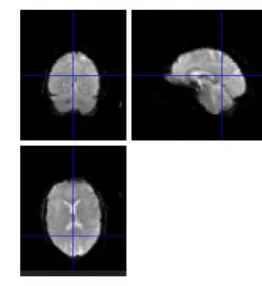
The fMRI data contain a lot of noise and artifacts resulted from heart-beat, breathing, head motion and the MRI acquisition system. After applying the group ICA to the fMRI data for obtaining the independent components, each component needs to be evaluated and the problematic components resulted from the artifacts in fMRI data should be excluded. In other words, in order to select the best components of the fMRI data, all the independent components and their corresponding time courses are required to be visually inspected. There are two main criteria for selecting the proper independent components of fMRI data for further analysis as follow,

24 1)Spatial feature of component

The independent component (IC) spatial maps should be inspected visually for us to be able to decide on keeping or excluding each component. First, the independent components and their peak activations should be in grey matter (GM) area for being qualified to be considered as the proper components. In other words, the components located in white matter (WM), cerebrospinal fluid (CSF) or those having overlap with brain arteries should be excluded. Also, the components located near brain edges and those with ring-like shape are due to the head motion artefact and should be excluded in the component selection process [51].

2)Time-course and power spectra

Inspecting the time-courses (TCs) corresponding to the independent components can also help us to find out which independent components are resulted from the artifact and should be excluded. In BOLD signals, the highest power is between 0.01 - 0.1 Hz. Hence, one of the main criteria to decide if a time-course indicates a BOLD-related signal is to inspect the presence of low frequency power. Power spectra of TCs should exhibit low frequency power with presence of the highest power between 0.01 – 0.1 Hz. However, sometimes the physiological noise due to cardiac pulsation (~ 1 HZ) or respiratory cycles (~ 0.3 HZ) becomes aliased into the low frequency fMRI time-course [51].

25

2.7 Dynamic Functional Brain Connectivity

The simplest way to investigate the degree to which each component is functionally related to the other components is to capture the pairwise Pearson correlation between the corresponding time-courses. By considering 𝑁 different brain components, a 𝑁 × 𝑁 symmetric matrix of connectivity can be obtained. Each element of this matrix is the correlation value between the time-courses of each pair of the components. Figure 2.9 shows an example of a connectivity matrix. Since the matrix of connectivity is a symmetric matrix, it has 𝑁 × (𝑁 − 1)/2 unique features. In connectivity matrix, the components based on their functional and anatomical location are grouped to form some networks such as auditory network, visual network, sensorimotor network and so on. The positive value of the correlation between the time-courses corresponding to a pair of brain regions is shown by the red color in Figure 2.9. Also, the negative correlation is represented by the blue color. If we calculate the correlation between the whole length of the time-courses corresponding to each pairs of the brain regions, the resulting correlation matrix would show the static functional connectivity.

Figure 2.9. An example of the brain functional connectivity matrix. The independent brain components are separated into seven groups. Sub-cortical (SC), auditory (AUD), visual (VIS), sensorimotor (SM), cognitive control (CC), default mode (DM) and cerebellum (CB).

26

As mentioned before, by studying the static functional connectivity, we are unable to understand the changes in the functional connectivity within the time. In 2013, Allen et al. [8] published one of the first major works on capturing dynamic functional brain connectivity. In this work, the functional connectivity was measured by using a set of temporal windows. Hence, for obtaining dynamic functional connectivity, a sliding window was applied to the time-courses, and then the correlation matrix was calculated inside each window as shown in Figure 2.10. In other words, first, by considering the length of window as 𝑊, the correlation matrix is calculated from time

𝑡 = 1 to time 𝑡 = 𝑊. Then, by shifting the window by time 𝜏 repeatedly, the same calculation is carried out in each window over the time, from the beginning of time-courses to the end of the time-courses. Considering length of window 𝑊 to be too short leads to the reduction of the signal to noise. It also results in having few samples for a reliable computation of correlation. In contrast, by having the long window length, we would not be able to detect the temporal changes in dFC. In other words, the length of window must be short enough to capture all the variations in dFC and long enough to get the reliable information of correlation. The size of 30–60s for the windows are suggested by the most studies for capturing the changes in resting-state dFC [1]. It also has been shown that, in most cases, different window lengths, when chosen in this interval, do not give significantly different results. Beside choosing the window length, defining the shape of the window is important. The most basic window is the common rectangular window. The limitation of using this window is that it has high the sensitivity to the outliers in the detection of dFC. To overcome this limitation tapered windows were used in many studies for capturing dFC. The size of the sliding window (tapered window) can be chosen based on the periodic behavior of the time courses. By using these sliding windows, it is possible to evaluate the amount of variability in the resulting FC time series.

27

Figure 2.10. Obtaining the functional connectivity matrices by using a sliding window [52]. .

2.8 K-means Technique

K-means is a well-known technique used for clustering the data [53]. This clustering technique has been used in different fields and applications for separating the data such as image segmentation and market segmentation. In k-means algorithm, 𝐾 non-overlapping clusters with 𝐾

centroids are picked and then each sample of the data is assigned to the nearest centroid. The centroids are estimated in such a way to minimize the total error. The error for each sample is defined as a function that measures the distance between a sample and its cluster centroid. The basic k-means algorithm for finding 𝐾 clusters is applied by following the steps given below,

28

Figure 2.11. K-means clustering fails to put image (b), (c) and (d) in the same cluster as image (a) [54].

(a) (b) (c) (d) 1. Select 𝑲 points (samples) as the initial centroids.

2. Assign all the samples to the closest centroid.

3. Recompute the centroid of each cluster.

4. Repeat steps 2 and 3 until the centroids don’t change (or change very little).

Even though the k-means is a well-known clustering method and has very simple implementation, it is worth mentioning one of its disadvantages. K-means clustering might not be well-suited for clustering of high dimensional data such as images. It results from the fact that using the distance measures such as Euclidian distance over the high dimensional spaces is not intuitive. For instance, in the case of the high dimensional images, k-means considers the pixel-wise distance for clustering the images that does not correspond to perceptual or semantic distance. Figure 2.11 shows an example that k-means clustering might fail, and the original image and three other images might fall into the different clusters based on their pixel-wise distance while we expect them to be in the same cluster based on their perceptual or semantic similarity.

29

(2.9)

2.9 Two Sample T-Test

T-statistics is a statistical method that is employed for comparing the means of two groups and assessing if this two groups are different or not. In other words, this method helps to investigate the degree of difference between two groups and the possibility that this difference could have happened by chance. This degree of difference is obtained based on: 1- The distance between the mean intensities of the two groups and 2- The spread of distribution of each group and the degree of overlap in distributions. As shown in Figure 2.12.

T-value is computed as,

𝑡 =

𝜇

− 𝜇

√

𝑠

𝑛

+

𝑠

𝑛

where 𝜇₁and 𝑠₁2 are the mean and sample variance of group 1, whereas 𝜇₂ and 𝑠₂2 are the mean and sample variance of group 2. Every value has a corresponding p-value. The p-value for a t-statistic gives the probability that the difference between two groups happens by chance.

𝜇₁ 𝜇₂

30

2.10 Summary

The purpose of this chapter was to present some background materials in study of the functional brain connectivity in the resting state fMRI. First, we explained how to preprocess and prepare the fMRI data. Then, group ICA which is an extension of ICA method was introduced. We explained how to use group ICA to capture independent components in this study. Then, we discussed how to choose appropriate components and exclude the artifact components. After that, we explained about functional connectivity matrix and how to capture dynamic functional connectivity using sliding windows. Finally, the two-sample t-test method for obtaining group difference was described.

31 Preprocessed fMRI data

Figure 3.1. The pipeline of dynamic functional brain connectivity study.

CHAPTER 3

Group Difference Study Using Convolutional Autoencoder

3.1 Introduction

In this chapter, we study the dynamic functional brain connectivity in fMRI data by using a convolutional autoencoder for obtaining the different connectivity patterns. A brief introduction of artificial neural networks is given in Section 3.2. The convolutional neural networks as a type of neural networks used for 2D data are described in Section 3.3. In Section 3.4, the convolutional autoencoders and their architecture are explained. In Section 3.5, we present the steps carried out to obtain dynamic functional connectivity. First, we apply the group ICA technique on the preprocessed resting-state fMRI data to get the independent components of fMRI data (brain regions) and the corresponding courses. A sliding window is then passed through the time-courses and a correlation matrix is obtained for each segment of the time-time-courses. As our main contribution, we use a convolutional autoencoder for the first time in order to obtain the correlation matrices with the common functional connectivity patterns. By using these connectivity patterns, we are able to study the differences in the functional connectivity in brain regions of the healthy control subjects and that of patients. The Figure 3.1 shows the pipeline for studying the dynamic functional connectivity. Group ICA and Windowing Autoencoder and Clustering Group Analysis

32

Figure 3.2. The physiological representation of a neuron [57].

3.2 Introduction to Neural Networks

Our brain uses the extremely large interconnected network of neurons for information processing. A neuron, such as the one shown in Figure 3.2, collects inputs from other neurons using dendrites. The neuron sums all the inputs and is fired if the resulting value is greater than a threshold. The signal from the fired neuron is then sent to other connected neurons through the axon.

Artificial neural network (ANN) is a computing system inspired by the brain neural networks [56]. An artificial neural network is a function (f: 𝑍→ 𝑂) that takes each sample from the input data 𝑍

and maps it to an output, 𝑂. This mapping is carried out by making meaningful connections between a number of neurons. Each neuron in a neural network gets a value determined by a weighted sum of all the inputs followed by an activation function [58] as shown in Figure 3.3. Activation function plays an important role in the artificial neural networks. The activation function decides whether a neuron should be activated or not. So, for each neuron 𝑗 in the network, its output 𝑂_𝑗 is defined as:

33

Figure 3.4. The most common activation functions [59]. Figure 3.3. The computation in a neuron.

. . . 𝑧1 𝑧2 𝑧₃ 𝑧𝑛 𝑂𝑗 𝑤_1𝑗 𝑤4𝑗 𝑤3𝑗 𝑤2𝑗 (3.1)

𝑂

= ∅(∑

𝑤

𝑧

+ 𝑏

)

where ∅ is the activation function, 𝑛 is the number of inputs to neuron 𝑗, 𝑤_𝑖𝑗 is the weight between neurons 𝑖 and 𝑗, and 𝑏 is the bias value. The commonly used activation functions in neural networks are Sigmoid, Tanh and ReLU as shown in Figure 3.4.

∑ +𝑏𝑗

∅

34

(3.2)

A neural network consists of a sequence of layers. Each layer uses the output of its previous layer as the input. Figure 3.5 shows a simple multi-layer neural network. Beside input and output layers, other layers of the network are called hidden layers. The input data are processed using the hidden layers and the results are passed to the output layer. In fact, the neural network maps the input data in the first layer to a set of prediction scores in the output layers using a set of weights in each layer. A cost function is defined to quantify the agreement between the prediction scores at output layer and the expected output (ground truth labels). Mean square error and cross entropy cost function are the most popular cost functions used in the neural networks. The weights of the neural network should be adjusted during training in such a way that minimize this cost function. In order to minimize the cost function, the weights in the neural network are optimized using a method called backpropagation. Backpropagation is a method used for training a neural network by calculating a gradient that is needed for updating the network weights. This process is carried out by computing the error at the output and distributing it backwards throughout the network layers. During the backpropagation, each weigh of the network is updated using the gradient descent as given by,

𝑤

= 𝑤

− 𝛼

𝜕𝐽

𝜕𝑤

where 𝑤𝑖𝑗 is the weight between neurons 𝑖 and 𝑗, 𝐽 is the cost function of the neural network and

𝛼 is the learning rate used for updating the weight. In fact, the gradient descent is a way to minimize the cost function 𝐽 parameterized by the model weights by updating the weights in the opposite direction of the gradient of the cost function with respect to the weights. The learning rate 𝛼

determines the size of the steps that is taken in the gradient descent direction to reach to the local minimum of cost function. Stochastic gradient descent (SGD) is a variation of gradient descent

35

Figure 3.5. A typical structure of a multi-layer neural network. Output Layer Input Layer

Hidden Layers

that estimates the gradient from a small number of samples chosen randomly from training data in each iteration (minibatches). SGD converges much faster than the original gradient descent in which all the data in the training set are used for estimation of the gradient in each iteration. Hence, SGD is used more often for training the neural network.

3.3 Convolutional Neural Networks

Convolutional neural network (CNN) is a type of neural networks that is typically used for 2D data such as images. The architecture of a Convolutional neural network is inspired by the organization of the Visual Cortex in which the individual neurons respond to stimuli in a restricted region of the visual field known as the receptive field. The convolutional neural network takes advantage of spatial structures in the input data by convolving a kernel to the input data to detect local features

36

Figure 3.6. A typical architecture of a convolutional neural network [60].

of the input [59]. Since the same kernel with the same parameters is used on every unit of the input data (parameter sharing), the number of parameters required to train a neural network drastically decreases. The convolutional neural network learns the feature representations of the input in each layer in a hierarchy by obtaining the low-level features in first layers and high-level features in the last layers. A typical convolutional neural network is shown in Figure 3.6. A convolutional neural network consists of two main building blocks called convolutional layers and pooling layers.

3.3.1 Convolutional Layer

The convolutional layer is the main building block of a convolutional neural network. In a convolutional layer, the convolution is performed by sliding a kernel over the input and carrying out a matrix multiplication and summation. A set of kernels is used in each convolutional layer to extract different kinds of features from the input data [61] and generate the layer output, called feature map. Stride and zero-padding are two important properties of each convolutional layer.

- Stride: Stride isthe number of steps by which we slide the kernel over the input image. When the

stride is 1 then we move the kernels by one step at a time. Using a larger stride leads to have smaller feature maps at the output of the layer.