Predicting Global Irradiance Combining Forecasting Models Through Machine Learning

This is a postprint version of the following published document:

Huertas-Tato, J., Aler, R., Rodríguez-Benítez, F.J.,

Arbizu-Barrena, C., Pozo-Vázquez, D. y Galván, I.M. (2018). Predicting

Global Irradiance Combining Forecasting Models Through

Machine Learning. In

HAIS 2018: Hybrid Artificial Intelligent

Systems,

10870, pp. 622-633.

DOI:

https://

doi.org/10.1007/978-3-319-92639-1_52

Predicting Global Irradiance Combining

Forecasting Models Through Machine

Learning

J. Huertas-Tato1(B)_{, R. Aler}1_{, F. J. Rodr´ıguez-Ben´ıtez}2_{, C. Arbizu-Barrena}2_, D. Pozo-V´azquez2_{, and I. M. Galv´an}1

1 _{Computer Science Departament, Universidad Carlos III de Madrid, Madrid, Spain} [email protected]

2 _{Department of Physics, Universidad de Ja´en, Ja´en, Spain}

Abstract. Predicting solar irradiance is an active research problem, with many physical models having being designed to accurately predict Global Horizontal Irradiance. However, some of the models are better at short time horizons, while others are more accurate for medium and long horizons. The aim of this research is to automatically combine the predic-tions of four different models (Smart Persistence, Satellite, Cloud Index Advection and Diffusion, and Solar Weather Research and Forecasting) by means of a state-of-the-art machine learning method (Extreme Gra-dient Boosting). With this purpose, the four models are used as inputs to the machine learning model, so that the output is an improved Global Irradiance forecast. A 2-year dataset of predictions and measures at one radiometric station in Seville has been gathered to validate the method proposed. Three approaches are studied: a general model, a model for each horizon, and models for groups of horizons. Experimental results show that the machine learning combination of predictors is, on average, more accurate than the predictors themselves.

Keywords: Global irradiance forecasting

·

1

Introduction

A key issue to increasethecompetitiveness of thesolarenergy and to increase theirshareintheelectricsystemsistheimprovementofthereliabilityofthesolar energyforecasts.Inthelastyears,awiderangeofforecastingmethodologieshas been developed, with very different characteristics, such as the spatial and temporalresolutionortheirforecastinghorizon[1].

MachineLearning[2]hasplayedanimportantroleonimprovingsolarenergy forecasting[3, 4].Nevertheless,thereisstillroomforimprovement.Inthisregard, therehave beensome effortstocombinedifferent sourcesofinformation (obser-vations,camera,satellite,...)andtakeadvantageofthepossiblesynergies.

Forexample,realmeasuresandcamerahavebeencombinedusinganarti-ficial neural network optimized through a genetic algorithm [5]. [6] proposes a combination ofNAM (North American Mesoscale Model) with cloudiness infor-mationobtained fromsatelliteimages.Thismodelimprovesspatialresolutionof the NAM, while improving intra-day and 1-day predictions.A systembased in extreme learning machines optimized through evolutionary computation (coral reef algorithm) combines direct measures, radiosondes and NWP to obtain the dailypredictionofsolarirradiance[7].In[8],acombinedpredictionofcloudcover derivedfromasky-cameraandsatelliteoffersaforecastofuptothreehours.Ina similar way,a combinationofcloudinessestimation fromsatelliteand theNWP from European Center for Medium range Weather Forecasting (ECMWF) is proposed[9].Furtherresults[10]showthatthecombinationofstatisticalmodels and NWPis ableto reduce theforecasting errorat one hour horizons. In[11] a machinelearningblendingofirradianceforecastsusingaRan-domForestisused. Thisapproachcombinesthreemodels:theNAMmodel,theSREF(ShortRange EnsembleForecast)modelandtheGFSmodel.Arecentworkcombines satellite-derived, ground data, solar radiation, and total cloud cover to improve solar radiationforecastingforhorizonsbetween1hand6h[12].

Similarcombinationapproaches have alsobeen appliedfor windenergy.[13] combines different predictions at several horizons using an adaptive weighting, dependentontheerroryieldedbythepastsources.

The novelty of this research is to use machine learning to combine Global HorizontalIrradiance(GHI)forecastsobtainedfromfoursources,inorderto out-put animprovedGHIforecast.Thesourcesare:SmartPersistence[14],Satellite [15], Cloud IndexAdvection and Diffusion (CIADCast) [16], and Solar Weather Research and Forecasting (WRF-Solar) [17]. These perform differently under different situations and forecasting horizons. Theaim of our approachis to use machinelearningtocombinethemautomatically,soastotakeadvantageoftheir synergiesandtoimprovetheperformanceofsourcesusedseparately.

Inthiswork,severalpredictionhorizonshavebeentestedfrom15to360min, instepsof15min.Threedifferentapproachesareproposedforintegratingthefour sources: general, horizon-individual and horizon-group. The approaches are different ways to treatthe horizon information either by usinga singlegen-eral model valid for all horizons, by making specialized models for each horizon (horizon-individual),oracompromisebetweenboth(horizon-group).

Themachinelearningmethodchosenforcombiningthemisextremegradient boosting [18]. Gradient boosting has been used before in solar forecasting. For instance,[19, 20]usemeteorologicalvariablestopredictGHI.However,theaimof ourworkisdifferent,becauseourinputsarenotmeteorologicalvariablesbutGHI forecaststhemselves.

Thestructureofthepaperisthefollowing:first,thepredictorsusedasinputs ofmachinelearningmethodarepresentedinSect.2.InSect.3,thedatasetusedto the evaluation is described. Section 4 explains the different machine learning approachestobestudiedinthiswork.InSect.5,theexperimentalmethodology

isexplainedandtheexperimentalresultsarepresented.Thefinalconclusionsof thisresearchandfuturelinesofworkarepresentedinSect.6.

2

Description

of

the

Predictors

This section describes the four forecasting models (or predictors) that will be combinedby amachinelearningmodel.

2.1 Smart Persistence

This model is computed with the actualmeasured irradiance I₀ and corrected with the variation of the clear-sky (cs) irradiances Ics from the initial time to

a future time t. The relation between actual irradiance and cs irradiance at a certain time 0 is kept constant and multiplied by the clear-sky irradiances in future t.TheEuropeanSolarRadiation Atlas[14]csmodelisused(Eq.1).

I(t) = I0 Ics(0)∗

Ics(t) (1)

2.2 Satellite-Based Model

Inthis method,satelliteimages arefirst processedtoderive theso-calledcloud indeximages,anintermediatesteptoretrievetheclear-skyindeximagesandthen the solar radiation maps [21]. Secondly, a statistical comparison of various consecutivecloudindeximagesallowsderivingthecloudmotionvectorfield.In this case OpenPIV is used (http://www.openpiv.net/openpiv-python/). The discrete cloud motion vector field is transformed into a continuous flow com-putingthestreamlines,i.e.,afamilyofcurvestangenttothiswindfield[15].The streamlinepassingthroughthestationlocationisusedtoobtainthefuturecloud indexvalues,thentheclear-skyindexvaluesand,finally,theGHIforecast

2.3 CIADCast

TheCIADCastmodel[16]forshort-termsolarradiationforecasting isbasedon theadvectionanddiffusionofcloudindexestimatesderivedfrom satelliteusing theWeatherResearchandForecasting[22]NWPmodels.Cloudindexvaluesare insertedintheWRFcellwhichcorrespondstothecloudtopheightprovidedby the EUMETSAT product.Then, WRF is used to advect and diffuse thecloud indexvaluesasdynamicaltracersbothhorizontallyandvertically.

Afterthe modelrun, thesumof each column of cloudindex values is com-putedtoobtainagainatwo-dimensionalcloudindexmap.Thecloudindexvalues atthestationlocationareusedfinallytoderivetheGHIforecast,similarlytothe satellite-basedmodel.CIADCastwasrunwiththestandardWRFmodelversion 3.7.1,configuredwith37verticallevels andthreenesteddomainsof27,9 and3 kmspatialresolution. Thecloudindexmapswereingestedintheinnerdomain, which has similar resolution to thesatellite images. 18-h simulations were run discardingthefirst6simulatedhoursasspin-up.

2.4 WRF-Solar

NWPusesmathematicalmodelsbasedonphysicalprinciplesoftheatmo-sphere and oceans to predictthe weatherbasedoncurrent weatherconditions. WRF-Solar [17] is a particularphysical configurationofthe WRF numericalweather prediction model version 3.6 devised for solar energy applications. It has improvedparameterizationsfortheinteractionsofsolarradiationwithcloudsand aerosols.Themodelconfigurationusedhereconsistedoftwonesteddomainswith 9 and 3 km spatial resolution and 37 vertical levels. As with CIADCast, simulationswith18hofforecastinghorizonand6hofspin-upwererun.

3

Data

The evaluation is conducted at one radiometric station in Seville (southern Spain)whereGHI(thetotalamountofshortwaveradiationreceivedfromabove byasurfacehorizontaltotheground)hasbeenmeasured.GHIhasbeenacquired with aKipp &ZonenCMP6pyranometerwitha 1minsamplerate.The main-tenance of radiometricstations follows World Meteorological Organization rec-ommendationsandthequalitycontrolofthedataisappliedfollowingLongand Dutton[23]. TheobservationscoverfromMarch2015to March2017.

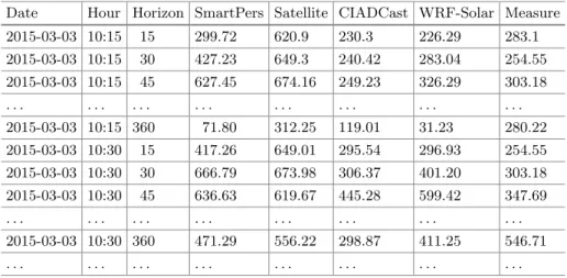
To ensure the quality of the data, a preprocessing of the dataset has been made.Onlypredictionstakenwhenthezenithislessthan75◦areincludedinthe dataset,becausethehoursselectedbythisfilterarethemostrelevantto global irradiancein theday.Forecasts ofGHI upto 6 hahead, witha timestepof 15 min, are obtained basedon four different models: Smart Persistence, Satellite-based,CIADCast,andWRF-Solar.Anexampleofthestructureofthedatasetis shownin Table 1.There arefour differentnumerical inputs(fourpredictors),a target(measurecolumn).Onaverage,eachhorizoncontains2400instances,

Table1.Datasetexample

Date Hour Horizon SmartPers Satellite CIADCast WRF-Solar Measure 2015-03-03 10:15 15 299.72 620.9 230.3 226.29 283.1 2015-03-03 10:15 30 427.23 649.3 240.42 283.04 254.55 2015-03-03 10:15 45 627.45 674.16 249.23 326.29 303.18 . . . . 2015-03-03 10:15 360 71.80 312.25 119.01 31.23 280.22 2015-03-03 10:30 15 417.26 649.01 295.54 296.93 254.55 2015-03-03 10:30 30 666.79 673.98 306.37 401.20 303.18 2015-03-03 10:30 45 636.63 619.67 445.28 599.42 347.69 . . . . 2015-03-03 10:30 360 471.29 556.22 298.87 411.25 546.71 . . . .

althoughthedistributionofthenumberofinstancesperhorizonisnotuniform (shorthorizonshave moreinstancesthanlonghorizons).

4

Methods

The approach to predict GHI is to combine a set of n predictors by means of machinelearningmodels,whichtheaimtoimprovethefinalpredictionforevery forecast horizon.Therefore, theGHIcan bedescribedby Eq.2,wheremachine learningmodelfisusedtocombineseveralpredictorsPi.:

ghi=f(P1, P2, ..., Pn) (2)

Inthisworktherearefourpredictorsavailablewhichareusedas inputsforthe machine learning algorithm. The predictors combined in this work have been describedin detailin Sect.2.Themachinelearning methodforfindingf is the extreme gradient boosting tree ensemble (xgbtree) [18]. This decision hasbeen takenaftercomparingpreliminaryresultswithrandomforestsandsupportvector machines.Xgbtreedisplayed agoodperformance, whileat thesame timeit isa very fast and efficient implementation. Inany case, other methods could have beenusedwithintheschemaproposedinthisarticle.

Giventhat eachpredictor performancedepends onthehorizon,three differ-ent approaches for dealing with horizons have been studied: general, horizon-individual,andhorizon-group.Theyaredescribedinthefollowingsubsections. 4.1 General Model

Thefirstapproachconstructsamodelthatminimizeserrorforallhorizons con-sideredtogether.Thisisachievedbycombiningdatafromthedifferenthorizons (i.e.excludingthehorizoncolumninTable1),andtrainingasinglemodelffrom thejointdataset.Equation3showshowmodelfcanbeusedforforecastingGHIat timetforhorizonh.Itcanbeseenthatfiscommonforallhorizons.

ghi(t+h) =f(P1(t, h), P2(t, h), ..., Pn(t, h)) (3)

4.2 Horizon-Individual Model

Thesecondapproachbuildsadifferentmachinelearningmodelfhforeach

hori-zon h. Each fhistrainedusingdata fromeachhorizon honly.Theend result

willbeasetof25machinelearningmodelsspecializedinpredictingGHIforevery singlehorizon. There isa modelfor horizon 15, ableto predict GHI at 15min forward in time, another model for horizon 30, ableto predict GHI at 30 min forward intime, andso on.Equation4 showshowto usemodelsfhfor making

GHIforecastsattimetforeachhorizonh.

ghi(t+h) = ⎧ ⎪ ⎪ ⎪ ⎨ ⎪ ⎪ ⎪ ⎩ f15(P1(t,15), ..Pn(t,15)), h≡15 f₃₀(P₁(t,30), ..P_n(t,30)), h≡30 ... f360(P1(t,360), ..Pn(t,360)), h≡360 (4)

4.3 Horizon-Group Model

This lastapproachbuildsa setofmodels,thistime byusinggroupsof horizons instead of individual horizons (as in the previous approach). Given that some predictors work better forclose horizons (SmartPersistence and Satellite) and othersformediumorlonghorizons(WRF-Solar),theaimistoidentifygroupsof horizons forwhich some predictors arebetter thanothers. Theadvantage over the horizon-individual approach is that noweach group of horizons have more data for training. The end result will be g machine learning models, each one specialized in predicting GHI for a horizon group, where g is the number of groups. Eachgroupmodelistrainedusingdatafromhorizonsbelongingtothat group only. This model is represented by Eq. 5, where the pi’s represent the

partitionpointsinthehorizonrangeandthe15≤h≤p1,p1 ≤h≤p2, . . . , pg−1≤h≤360 are theghorizon groups.

ghi(t+h) = ⎧ ⎪ ⎪ ⎪ ⎨ ⎪ ⎪ ⎪ ⎩ f1(P1(t, h), ..Pn(t, h)), 15≤h≤p1 f2(P1(t, h), ..Pn(t, h)), p1≤h≤p2 ... fg(P1(t, h), ..Pn(t, h)), pg−1≤h≤360 (5)

After visual analysis and taking into account the performance of the fore-casting modelsfor thedifferent horizons, three groups(g =3) have beenused, althoughlarger valuescouldbeconsideredat theexpenseofcomputationalcost anddiminishingthenumberofdataforeachgroup.

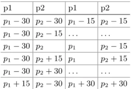
Inordertodecidetheactuallocation ofp₁ and p2,a greedysearchhasbeen implemented.Startingfromsomeinitialvaluesforp₁ andp2,allcombinationsof neighboring pointsareexplored.Thesetofneighbors of(p1,p2)isconsideredto be (p₁ ±0, 15,30, p₂ ±0,15,30). Table2 showsthose neighboringpoints. For eachpartitionexplored,threedifferentmodelsareobtained(onepergroup),each onetrainedwithdatafromeachhorizongroupandevaluatedonvalidationsets. Outofalltheneighbors,thefourcombinationswithlowesterrorsarekept.

Thereasonforkeepingmorethanone(p1,p2)combinationistoavoidfalling intolocalminima.Thecombinationwithlowesterror,andstillunvisitedbythe algorithm,isthenextexploredcombinationofpoints.p1 andp2 arethenupdated to those locations that minimize the average validation error. This process is repeated until there is an empty list of combinations or the 4 best possible combinationshavealreadybeenexplored.Attheendofthesearch,thealgorithm chooses the partition (i.e. combinationof p1 and p2)with the besterror found throughoutallthesearch.

Themethodisdetailed inAlgorithm1.Line1 createsatable(VisitedTable) that stores information about all combinations (p1, p2) explored by the algo-rithm.Thatis,Accuracy istheaverage validationerrorforeachparticular com-bination; visited informs whether this combination has already been explored; and lastVisit marks one of the pairs as the one that should be selected for expandingtheneighbors.

Table 2.Neighbors for anyp₁ andp₂ p1 p2 p1 p2 p1−30 p2−30 p1−15 p2−15 p1−30 p2−15 . . . . p1−30 p2 p1 p2−15 p1−30 p2+ 15 p1 p2+ 15 p1−30 p2+ 30 . . . . p1+ 15 p2−30 p1+ 30 p2+ 30

Loopin lines2–17runswhileitispossibletofindcombinationsthat improve theerror.Inline3 thelaststateisretrievedfromVisitedTable(i.e.lastVisit== TRUE).Afterbeingretrieved,lastVisitwillbesettoFALSE.Inline4,the(p1,p2) combinationisretrievedfromLastStateandallpossibleneighborsarecalculatedin line 5 (AllNeighbours(p1, p2)).The loop in lines6–12 checksevery pairof points fromthelistofneighbors(seeTable2)previouslyexpanded(NewPointList).Ifthe pair has already been visited, it can be extracted out of the VisitedTable. Otherwise,itsperformanceiscomputed(Accuracy(p1, p2))inline10.Attheendof theloop,PairErrorscontainstheperformanceofallneighbors.Line13selectsthe bestfourcombinations(BestErrors),outofwhichthebestunvisitedpairisfinally selected(line14).ThisbestpairismarkedwithlastVisit=TRUE,sothatitwill be selected in the next iteration for computing neighbors. All information regarding new explored pairs and their respective errors is included into VisitedTable(line15).Explorationwillcontinue,asfarasatleastoneofthefour best pairswas unvisited (BestError not empty, line 18). Once thetermination conditionissatisfied,thebestpair(p1,p2) from VisitedTableisreturned.

Algorithm 1. Horizon-group greedy search process

1:V isitedT able←Table(p1, p2,Accuracy(p1, p2), visited, lastV isit)

2:whilecontinuedo

3: LastState←lastV isitinV isitedT ableisT RU E

4: p1, p2←p1andp2inLastState

5: N ewP ointList←AllNeighbours(p1, p2)

6: foreachP ointP airinN ewP ointListdo

7: ifp1, p2exists inV isitedT able then

8: P airError←errorinV isitedT able

9: else

10: P airError←Accuracy(p1, p2)

11: end if

12: end for

13: BestErrors←select 4 lowest fromP airErrors

14: BestError←select lowest and !visitedfromBestErrors. Mark this pair withlastV isit←

T RU E

15: updateV isitedT ablewithN ewP ointListandP airErrors

16: continue←!(BestErroris empty)

17: end while

5

Experimentation

Theaimoftheexperimentationistocomparetheskillofeachmethodpre-sented here topredictGHI ateachhorizon fromh = 15 toh=360. Thereareseven different methods to compare, four of them are the predictors (WRF-Solar, CIADCast,SmartPersistenceandSatellite)andtheotherthreearethedifferent machinelearningapproachesproposedinthiswork(General,Horizon-individual andHorizon-group).

5.1 Methodology

Thedatasetisdividedintotwosubsets:trainingandtest.Theformerismadeup ofthe21firstdaysofeachmonth(3weeksofdata),thelatterisforthetestset, thatwillbeusedtoevaluatethetrainedmodel.Thetrainingsetitselfisdivided intoamodel-trainingsetandavalidationset. Thefirstonecontainsthe14first daysofthemonthanditisusedfortrainingthemodels.Thevalidationsetisused forhyper-parametertuningandtoguidethesearchprocessforthehorizon-group approachandtoselectthebesthorizongroups(seeSect.4.3).Themetricusedfor comparison purposes is the normalized root mean square error, which is calculatedinEq.6. nRMSE= _(x i−oi)2/N _(o i)/N (6) where xi is a prediction, oi is an observationand N is thenumber of samples.

nRMSE is calculated for each horizon. The global nRMSE is the mean of all horizon nRMSEvalues.

5.2 Results

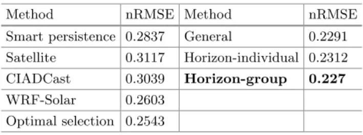
InTable 3 theglobaltest nRMSE foreach modelisshown. Thefirstfour rows refertothepredictors.Thefifthrowdisplaystheerrorthatwouldbeobtainedif foreachhorizon,thebestpredictorwouldbeselected(calledoptimalselectionin Table 3). Given that this selection is done using the test set, it could not be appliedinpractice.Itisprovidedonlyforcomparisonpurposeswiththemachine learning approaches.It can beseen that all machine learning approaches have betterglobalerrorthananyofthepredictorsoreventheiroptimalselection.On average,WRF-Solaristhemostreliablepredictor(0.2603globalnRMSE), with SmartPersistencebeingthesecondbest(0.2837nRMSE).Observingthemachine learning blending approaches, the most accurate prediction method is the horizon-groupapproachwithaglobalnRMSEof0.227.AfterapplyingAlgorithm 1,horizongroupsare15–60,75–270and285–360.

Table4 shows thenRMSE broken downby horizon (fromh= 15 to h= 360)foreachofthedifferentpredictorsandapproaches.Thisinformationisalso displayed in Figs. 1 and 2. Figure 1 compares the predictors. Under an hour, CIADCastisthebestpredictoravailable,thenSmartPersistenceisbestuntil

Table 3.Global nRMSE

Method nRMSE Method nRMSE Smart persistence 0.2837 General 0.2291 Satellite 0.3117 Horizon-individual 0.2312 CIADCast 0.3039 Horizon-group 0.227

WRF-Solar 0.2603 Optimal selection 0.2543

90 min, when WRF-Solar starts being the best model from that point onwards. There are a couple of times where WRF-Solar is worse, at 105 and 150 min. Interestingly, for WRF-Solar, the nRMSE decreases as h increases, although after 285 min the error starts increasing again.

Table 4.nRMSE by horizon

h= 15 30 45 60 75 90 105 120 135 150 165 180 General 0.197 0.205 0.211 0.217 0.226 0.229 0.22 0.217 0.219 0.215 0.216 0.225 h-individual 0.208 0.21 0.213 0.221 0.234 0.229 0.22 0.217 0.225 0.223 0.22 0.227 h-group 0.203 0.208 0.209 0.212 0.228 0.23 0.222 0.218 0.218 0.217 0.216 0.226 CIADCast 0.229 0.244 0.252 0.263 0.283 0.287 0.281 0.29 0.297 0.282 0.273 0.270 Satellite 0.229 0.248 0.255 0.26 0.288 0.298 0.291 0.28 0.268 0.267 0.275 0.289 SmartPer 0.245 0.252 0.255 0.259 0.274 0.28 0.265 0.271 0.281 0.281 0.276 0.293 WRFSolar 0.284 0.272 0.279 0.277 0.284 0.274 0.269 0.264 0.262 0.268 0.266 0.265 h= 195 210 225 240 255 270 285 300 315 33 345 360 General 0.22 0.221 0.22 0.233 0.236 0.234 0.232 0.246 0.261 0.275 0.264 0.260 h-individual 0.226 0.227 0.223 0.226 0.241 0.234 0.225 0.241 0.264 0.271 0.256 0.269 h-group 0.22 0.224 0.217 0.231 0.234 0.23 0.227 0.244 0.256 0.257 0.255 0.248 CIADCast 0.264 0.291 0.301 0.312 0.356 0.348 0.337 0.353 0.358 0.372 0.37 0.381 Satellite 0.298 0.306 0.311 0.346 0.332 0.345 0.348 0.353 0.382 0.391 0.422 0.4 SmartPer 0.288 0.279 0.275 0.294 0.296 0.288 0.275 0.304 0.318 0.333 0.314 0.313 WRFSolar 0.263 0.253 0.251 0.237 0.229 0.242 0.231 0.237 0.254 0.26 0.264 0.263

InFig.2 themachinelearning approaches (General,Horizon-individualand Horizon-group) are compared to the optimal selection of predictors mentioned above.Allmachinelearningcombinationofpredictorsarebetterthanthe origi-nalpredictorsupto255min.Atthatpoint,itisdifficulttoobserveadifference respect to the predictors (WRF-Solar being the most accurate one at those horizons,asshowninFig.1). Themachinelearningapproachesshowminor dif-ferences.First,thehorizon-individualmodelisconsistentlyworseduringtheearly horizons, while both the general and horizon-groupmodels are similar in their performance.Howeverwhenthe255minhorizonisreached,theybecome

Fig. 1.Predictor performance at different horizons.

Fig. 2.Performance of the three machine learning approaches at different horizons.

harder to differentiate and behave similarly. At long horizons, starting at the 330 horizon, the horizon-group approach outperforms the other approaches and predictors. All machine learning models consistently increase in nRMSE as the horizon increases.

6

Conclusions

In this paper machine learning methods have been tested in order to combine GHI forecasting models (Smart Persistence, Satellite, CIADCast and WRF-Solar) as inputs to Xgboost, with the aim of improving predictions in horizons

from 15 to 360 min. Three approaches have been studied: a general approach that disregards horizon information, a horizon-individual approach that builds a Xgboost model for each horizon, and a horizon-group approach that separates horizons in three groups and builds a Xgboost model for each group. Experi-mental results show a great accuracy improvement over the predictors on short time horizons, and equivalent performance to the best predictor on further hori-zons. The general, horizon-individual and horizon-group models display similar performance, although for far horizons, the latter displays a better performance. Overall, the final results are satisfactory, showing that there is a lot of margin for improvement in the field of solar forecasting using machine learning. In the future, we would like to improve results further by including additional features, such as other predictors or historical solar radiation data. It can be also interest-ing traininterest-ing different models for different seasons or different weather regimes. Another interesting research work would be automatically selecting subsets of predictors for each horizons or groups of horizons.

Acknowledgments. The authors are supported by the Spanish Ministry of Econ-omy and Competitiveness, projects 1-R and ENE2014-56126-C2-2-R and FEDER funds. Some of the authors are also funded by the Junta de Andaluc´ıa (research group TEP-220).

References

1. Inman, R.H., Pedro, H.T.C., Coimbra, C.F.M.: Solar forecasting methods for renewable energy integration. Prog. Energy Combust. Sci.39(6), 535–576 (2013) 2. Witten, I.H., Frank, E., Hall, M.A., Pal, C.J.: Data Mining: Practical Machine

Learning Tools and Techniques. Morgan Kaufmann (2016)

3. Voyant, C., Notton, G., Kalogirou, S., Nivet, M.-L., Paoli, C., Motte, F., Fouilloy, A.: Machine learning methods for solar radiation forecasting: a review. Renew. Energy105, 569–582 (2017)

4. Terren-Serrano, G.: Machine learning approach to forecast global solar radiation time series (2016)

5. Chu, Y., Pedro, H.T.C., Coimbra, C.F.M.: Hybrid intra-hour DNI forecasts with sky image processing enhanced by stochastic learning. Sol. Energy 98, 592–603 (2013)

6. Mathiesen, P., Collier, C., Kleissl, J.: A high-resolution, cloud-assimilating numeri-cal weather prediction model for solar irradiance forecasting. Sol. Energy92, 47–61 (2013)

7. Salcedo-Sanz, S., Casanova-Mateo, C., Pastor-S´anchez, A., S´anchez-Gir´on, M.: Daily global solar radiation prediction based on a hybrid coral reefs optimization-extreme learning machine approach. Sol. Energy105, 91–98 (2014)

8. Alonso, J., Batlles, F.J.: Short and medium-term cloudiness forecasting using remote sensing techniques and sky camera imagery. Energy73, 890–897 (2014) 9. Lorenz, E., K¨uhnert, J., Heinemann, D.: Short term forecasting of solar irradiance

by combining satellite data and numerical weather predictions. In: Proceedings of 27th European Photovoltaic Solar Energy Conference, Valencia, Spain, pp. 4401– 440 (2012)

10. Huang, J.,Korolkiewicz,M.,Agrawal,M.,Boland,J.:Forecastingsolarradiation on an hourly time scale using a coupled autoregressive and dynamical system (cards)model.Sol.Energy87,136–149(2013)

11. Lu, S., Hwang, Y., Khabibrakhmanov, I., Marianno, F.J., Shao, X., Zhang, J., Hodge,B.M.,Hamann,H.F.:Machinelearningbasedmulti-physical-model blend-ingforenhancingrenewableenergyforecast-improvementviasituationdependent errorcorrection.In:EuropeanControlConference(ECC),pp.283–290(2015)

12. MazorraAguiar,L.,Pereira,B.,Lauret,P.,D´ıaz,F.,David,M.:Combiningsolar irradiancemeasurements,satellite-deriveddataandanumericalweatherprediction modeltoimproveintra-daysolarforecasting.Renew.Energy97,599–610(2016)

13. S´anchez, I.:Adaptive combination of forecasts with application to wind energy. Int.J.Forecast.24(4),679–693(2008)

14. Rigollier,C.,Bauer,O.,Wald,L.:OntheclearskymodeloftheESRA-European SolarRadiationAtlas-withrespecttotheheliosatmethod.Sol.Energy68(1),33– 48(2000)

15. Nonnenmacher,L.,Coimbra,C.F.M.:Streamline-basedmethodforintra-daysolar forecastingthroughremotesensing.Sol.Energy108,447–459(2014)

16. Arbizu-Barrena,C.,Ruiz-Arias,J.A.,Rodr´ıguez-Ben´ıtez,F.J.,Pozo-V´ezquez,D., Tovar-Pescador,J.:Short-termsolarradiationforecastingbyadvectingand diffus-ingMSGcloudindex.Sol.Energy155,1092–1103(2017)

17. Jimenez,P.A.,Hacker,J.P.,Dudhia,J.,Haupt,S.E.,Ruiz-Arias,J.A.,Gueymard,

C.A.,Thompson,G.,Eidhammer,T.,Deng,A.:WRF-solar:descriptionand clear-skyassessmentofanaugmentedNWPmodelforsolarpowerprediction.Bull.Am. Meteorol.Soc.97(7),1249–1264(2015)

18. Chen,T.,Guestrin,C.:XGBoost:ascalabletreeboostingsystem.In:Proceedings ofthe22ndACMSIGKDDInternationalConferenceonKnowledgeDiscoveryand DataMining,KDD2016,pp.785–794.ACM(2016)

19. Urraca,R.,Antonanzas,J.,Antonanzas-Torres,F.,Martinez-de-Pison,F.J.: Esti-mationofdailyglobalhorizontalirradiationusingextremegradientboosting machines.In:Gra˜na,M.,L´opez-Guede,J.M.,Etxaniz,O.,Herrero,A.,´ Quinti´an,H., Corchado,E.(eds.)ICEUTE/SOCO/CISIS-2016.AISC,vol.527,pp.105–113. Springer,Cham(2017).https://doi.org/10.1007/978-3-319-47364-211

20. Fan, J., Wang, X., Lifeng, W., Zhou, H., Zhang, F., Xiang, Y., Xianghui, L., Xiang,Y.:Comparisonofsupportvectormachineandextremegradientboosting forpredictingdailyglobalsolarradiationusingtemperatureandprecipitationin humid subtropical climates: a casestudy in China. Energy Conv. Manag. 164, 102–111(2018)

21. Rigollier,C.,Lef`evre,M.,Wald,L.:Themethodheliosat-2forderivingshortwave solarradiationfromsatelliteimages.Sol.Energy77(2),159–169(2004)

22. SkamarockWilliam,C.,Joseph,B.K.,Jimy,D.,David,O.G.,Dale,M.B.,Michael,

G.D.,Huang,X.Y.,Wang,W.,Jordan,G.P.:Adescriptionoftheadvancedresearch WRFversion3.NCARtechnicalnote,126(2008)

23. Long, C.N., Dutton, E.G.:BSRN globalnetwork recommendedQC tests,v2. x. (2010)