Improving the interpretability of classification rules discovered by an ant colony algorithm.

(1)

Improving the Interpretability of Classification Rules

Discovered by an Ant Colony Algorithm

Fernando E. B. Otero

School of Computing

University of Kent, Chatham Maritime Kent, ME4 4AG, UK

Alex A. Freitas

School of Computing University of Kent, Canterbury

Kent, CT2 7NF, UK

ABSTRACT

The vast majority of Ant Colony Optimization (ACO) al-gorithms for inducing classification rules use an ACO-based procedure to create a rule in an one-at-a-time fashion. An improved search strategy has been proposed in the c Ant-MinerPBalgorithm, where an ACO-based procedure is used to create a complete list of rules (ordered rules)—i.e., the ACO search is guided by the quality of a list of rules, in-stead of an individual rule. In this paper we propose an ex-tension of thecAnt-MinerPB algorithm to discover a set of rules (unordered rules). The main motivation for discovering a set of rules is to improve the interpretation of individual rules and evaluate the impact on the predictive accuracy of the algorithm. We also propose a new measure to eval-uate the interpretability of the discovered rules to mitigate the fact that the commonly-used model size measure ignores how the rules are used to make a class prediction. Compar-isons with state-of-the-art rule induction algorithms and the

cAnt-MinerPBproducing ordered rules are also presented.

Categories and Subject Descriptors

I.2.8 [Artificial Intelligence]: Problem Solving, Control Methods, and Search—Heuristic methods

General Terms

Algorithms

Keywords

ant colony optimization, data mining, classification, sequen-tial covering, unordered rules

1. INTRODUCTION

Ant colony optimization (ACO) has been successfully ap-plied to the classification task in data mining. Classification problems can be viewed as optimisation problems, where the goal is to find the best model that represents the predictive

Permission to make digital or hard copies of all or part of this work for personal or classroom use is granted without fee provided that copies are not made or distributed for profit or commercial advantage and that copies bear this notice and the full citation on the first page. To copy otherwise, to republish, to post on servers or to redistribute to lists, requires prior specific permission and/or a fee.

relationships in the data [19, 4, 25]. In essence, a classi-fication problem consists of discovering a predictive model that represents the relationships between the predictor at-tribute values and the class (target) atat-tribute values of data instances (also called examples, or cases). The discovered classification model is then used to classify—predict the class attribute value of—new examples (unseen during training) based on the values of their predictor attributes.

Since the introduction of Ant-Miner [18], the first ant colony rule induction algorithm for the discovery of a list of classification rules, many extensions have been proposed in the literature [7, 12]. The vast majority of these exten-sions follow the same overall design: they employ an ACO procedure to create a single classification rule in the form IF<term1 AND. . .AND termn>THEN<class value>at

each iteration of the algorithm, where the IF part corre-sponds to the antecedent of the rule and the THEN part corresponds to the consequent of the rule. The ACO-based construction procedure is repeated many times to produce a classification model (i.e., a list of classification rules). The strategy of creating one-rule-at-time, where the creation of each rule is an independent search problem, can lead to the problem of rule interaction—the creation of a rule affects the rules that can be created in subsequent iterations. A new strategy to mitigate the potential problem of rule inter-action has been recently proposed in [17] and implemented in thecAnt-MinerPBalgorithm. The main idea proposed in the new strategy is the use of an ACO procedure to create a complete list of rules and guide the search based on the quality of the whole list, therefore taking into account the interaction between the rules in the list.

This paper proposes an extension of the cAnt-MinerPB algorithm to create unordered rules. The main motivation is to improve the interpretation of individual rules. In an ordered set of rules (also referred to as list of rules), the effect (meaning) of a rule depends on all previous rules in the list, since a rule is only used if all previous rules do not cover the example. On the other hand, in an unordered set of rules, an example is shown to all rules and a single rule is used to make a prediction. We evaluate the new exten-sion, called UnorderedcAnt-MinerPB, against state-of-the-art rule induction algorithms in terms of predictive accuracy using 18 publicly available datasets. We also propose a new measure to evaluate the size of the discovered model and present the results obtained bycAnt-MinerPBand the pro-posed UnorderedcAnt-MinerPB algorithms.

The remainder of this paper is organized as follows. Sec-tion 2 presents a discussion of the new strategy implemented

(2)

in thecAnt-MinerPBalgorithm. The details of the proposed extension to create unordered rules are presented in Sec-tion 3. The computaSec-tional results are presented in SecSec-tion 4. Finally, Section 5 concludes this paper and presents future research directions.

2. BACKGROUND

The majority of ant colony classification algorithms fol-lows a sequential covering strategy in order to create classi-fication rules. The sequential covering strategy (also known as separate-and-conquer) is a commonly used strategy in machine learning to create a list/set of rules and it consists of two main steps: the algorithm creates a rule that clas-sifies part of the available training examples (conquer step) and then removes the classified examples (separate step). This iterative process is repeated until (almost) all exam-ples have been classified—i.e., there is a rule that classifies each of the available training examples. The use of the se-quential covering strategy reduces the problem of creating a list/set of classification rules into a sequence of simpler problems, each requiring the creation of a single rule. In the case of ant colony classification algorithms, a single rule is created by an ACO procedure, which aims at searching for the best rule given a rule quality function. This is the strategy found in Ant-Miner [18], the first ACO-based rule induction algorithm, and its many extensions [7, 12]. One of the few exceptions is the Grammar Based Ant Program-ming (GBAP) algorithm [15, 16], which does not follow the sequential covering. In GBAP, each ant in the colony cre-ates a rule using a context-free grammar and a list of rules is obtained using a niching approach—different ants compete to cover all training examples and the most accurate ones are used to compose a list of rules.

Recently, [17] proposed a new strategy to create classifi-cation rules using an ACO algorithm, implemented in the

cAnt-MinerPBalgorithm. The main motivation for the new strategy is to avoid the potential problem of rule interaction arising from the greedy nature of the sequential covering. Since rules are discovered in an one-at-a-time fashion in the sequential covering, the outcome of a rule (the examples re-moved by the rule) affects the remaining rules that can be created—the removal of the examples effectively changes the search space for the later iterations. As a result, Ant-Miner (and its variations) perform a greedy search for the list of best rules, using an ACO procedure to search for the best rule give a set of examples, and it is highly dependant in the order that rules are created. The strategy implemented in

cAnt-MinerPB mitigates the problem of rule interaction by using an ACO procedure to search for the best list of rules. Therefore, an ant incAnt-MinerPB creates a complete list of rules, while an ant in Ant-Miner creates a single rule.

In this paper we propose an extension tocAnt-MinerPB to discover unordered rules (set of rules) instead of ordered rules (list of rules), with the aim of improving the inter-pretability of the discovered rules. The discovery of un-ordered rule sets has been previously explored as extensions to the Ant-Miner algorithm only in [23, 14] to the best of our knowledge, although the search strategy of Ant-Miner and

cAnt-MinerPBare very different—both of the Ant-Miner ex-tensions in [23, 14] use an ACO procedure to create an indi-vidual rule. The motivation for extending thecAnt-MinerPB algorithm is to use an ACO procedure to search for the best

set of rules, taking advantage of the improved strategy im-plemented incAnt-MinerPB.

3. CREATING UNORDERED RULE SETS

cAnt-MinerPB creates a list of rules (also referred to as ordered rules), where the order of rules plays an important role in the interpretation of individuals rules. When using a list of rules to classify a new example, each rule is tested sequentially—i.e., the example is shown to the first rule, then the second, and so forth—until a rule that covers1

the example is found. Therefore, the effect (meaning) of a rule depends on all previous rules in the list, since a rule is only used if all previous rules do not cover the example. A simple example of this effect was given by [1]:

If feathers = yes then class = bird else if legs = two then class = human else ...

The rule ‘if legs=two then class=human’ cannot be cor-rectly interpreted alone, since birds also have two legs. If we analyse the rule in the context of the list, an example is going to be tested against it only if the first rule is not used. In the case of birds, they will satisfy the first rule and be classified correctly as ‘birds’. This problem becomes more complex when we consider larger lists of rules.

An alternative to improve the interpretation of individual rules is to create a set of rules (also referred to as unordered rules), where the order of rules is not important. The use of a set of rules to classify an example consists of finding all rules that cover the example. If only one rule covers the example, the rule classifies the example; if multiple rules cover the example, a conflict resolution criteria is used to decide the final classification of the example. Rule conflict resolution criteria will be discussed in Subsection 3.4.

3.1 Unordered

c

Ant-Miner

_PB

The main modification in order to create unordered rules is in the way ants create the set of rules. Instead of creat-ing a rule and then determine its consequent based on the majority class value of the covered training examples, the Unordered cAnt-MinerPB introduces an extra loop to iter-ate over each class value. Therefore, an ant creiter-ates rules for each class value in turn, using as negative examples all the examples associated with different class values. Figure 1 presents the high-level pseudocode of the Unorderedc Ant-MinerPBalgorithm.

In summary, the unordered algorithm works as follows. An ant starts with an empty set of rules (outer for loop). Then, it creates rules for each of the class values (inner for-all loop). An ant creates rules for a specific class value until all examples of the class have been covered or the number of examples remaining for the class is below a given max-imum threshold (innerwhile loop). After a rule is created and pruned, it is added to current set of rules and the train-ing examples correctly covered by the rule are removed—i.e., the examples covered by the rule that are associated with the rule’s class value (positive examples). The heuristic in-formation for the current class value is recalculated at each iteration to reflect the changes in the predictive power of 1

A rule covers an example when the example satisfies all the conditions in the antecedent of the rule.

(3)

Require: training examples Ensure: best discovered rules

1. _{InitialisePheromones()}_; 2. rulesgb←∅;

3. _m_←_0;

4. _while_{m <}_{maximum iterations}_and_{not stagnation}_do 5. rulesib←∅;

6. _for_n_←₁_to_{colony size}_do 7. _rules_n_←∅_;

8. _{for all}_class _in_classes_do

9. _examples_←_{all training examples}_;

10. _while_Count₍_examples_,_class₎_>_{maximum uncovered}_do 11. _{ComputeHeuristicInformation(examples, class)}_; 12. _rule _←_CreateRule₍_examples_,_class_);

13. _{P rune}₍_rule_);

14. _examples_←_examples₋_{Covered(rule, class, examples)}_; 15. rulesn←rulesn+rule;

16. _{end while}

17. _{end for}

18. _if Quality(rulesn)> Quality(rulesib)then

19. _rules_ib_←_rules_n_; 20. _{end if}

21. _{end for}

22. _{U pdateP heromones}₍_rules_ib_);

23. _if _Quality₍_rules_ib₎_{> Quality}₍_rules_gb₎_then 24. rulesgb←rulesib;

25. _{end if} 26. _m_←_m_{+ 1;} 27. _{end while} 28. _return rulesgb;

Figure 1: High-level pseudocode of the UnorderedcAnt-MinerPB algorithm.

the candidate terms due to the removal of the positive ex-amples. The examples associated with different class values (negative examples) remain, even the ones that are covered by a rule—unlike the original (ordered) cAnt-MinerPB al-gorithm, where all covered examples are removed. After creating rules for all class values, the iteration-best set of rules is updated if the quality of the newly created set of rules is greater than the quality of the current iteration-best set. Once all ants have created a set of rules and the iteration-best set is determined, the pheromone values are updated using the iteration-best set and the global-best set of rules is updated, if the quality of the iteration-best set is greater than the quality of the global-best set (i.e., the best set of rules produced so far since the start of the search). The entire procedure (outerwhile loop) is repeated until ei-ther a maximum number of iterations has been reached or the search has converged. At the end, the best set of rules found is returned as the discovered set of rules.

Note that when an ant is creating a rule, the consequent of the rule (the class value predicted by the rule) is fixed. Therefore, the heuristic information and the dynamic dis-cretization of continuous values take advantage of the class information and use a more accurate class-specific measure.

3.2 Class-Specific Heuristic Information

The heuristic information of each vertex vi of the

con-struction graph for the class valuecis given by

ηvi(c) =

|Examples(vi, c)|

|Examples(vi)|

, (1)

where|Examples(vi, c)|is the number of training examples

that satisfy the term (attribute-condition) represented by vertex vi and that are associated with class value c, and

|Examples(vi)|is the number of training examples that

sat-isfy the term (attribute-condition) represented by vertexvi.

In other words, the heuristic informationηvi(c) corresponds

to the fraction of training cases that are correctly covered by the termviwith respect to the class valuec.

3.3 Class-Specific Dynamic Discretisation

Continuous attributes represent a special case of vertices in the construction graph since they do not have a set of fixed intervals to define a complete term (attribute condi-tion). When a vertice representing a continuous attribute is used, either for computing heuristic information or during the rule construction process, a dynamic discretisation pro-cedure is employed to select a discrete interval in order to create a term. cAnt-MinerPBuses an entropy-based proce-dure, which does not require the class information a priori. Since in the unordered extension the class value is available to the discretization procedure, we use the Laplace accu-racy as a criteria to select a threshold value to discretize a continuous attribute as follows.

(4)

at-tributex dynamically generates two intervals: x ≤ t and

x > t. The best threshold value is the valuetthat maximises the interval accuracy in the set of examplesSregarding the class valuec, given by

max(Lap(c, Sx≤t),Lap(c, Sx>t)) ∀t∈Dx, (2)

whereSx≤t is the set of examples that satisfy the interval

x≤t, Sx>t is the set of examples that satisfy the interval

x > tandDx are the values in the domain of attribute x.

The Laplace accuracy of an interval is given by

Lap(c, E) =|Ec|+ 1

|E|+k , (3)

where E is the set of examples in the interval, |Ec|is the

number of examples inE that are associated with the class valuec,|E|is the number of examples inEandkis the num-ber of different values in the domain of the class attribute.

After selecting the best threshold valuet, a term for the continuous attributexis created based on the Laplace ac-curacy of the two intervals generated, given by

termx=

( _x_≤_t_{if Lap}₍_{c, S}

x≤t)>Lap(c, Sx>t)

x > tif Lap(c, Sx≤t)<Lap(c, Sx>t)

. (4)

3.4 Using a Set of Rules to Classify Examples

As aforementioned, in order to classify an example using a set of rules, all rules that cover the example are identified. The prediction of the class value of an example leads to one of the following scenarios:

1. None of the rules covers the example: the example is assigned the default class value, which corresponds to the majority class value of the training set;

2. Only one rule covers the example: the example is as-signed the class value predicted by the rule;

3. Multiple rules predicting the same class value cover the example: the example is assigned the class value pre-dicted by the rules;

4. Multiple rules predicting different class values cover the example: a conflict resolution strategy is used to de-termine the predicted class value. There are mainly two strategies: (i) use the rule with the highest qual-ity (rule selection strategy); (ii) combine (sum up) the class distribution of covered examples amongst the class values of each rule and predict the majority class value in the sum (rule aggregation strategy), as pro-posed in [1].

Let us consider an example in a 2-class problem{Y,N}that is covered by rules R1⇒Y [7,0], R2⇒Y [4,0] and R3⇒N [1,5](the values between squared brackets correspond to the class values distribution of the covered examples). Since

R3 predicts a class value different from the one predicted by R1 and R2, we have a conflict. If we use a class rule aggregation strategy to resolve the conflict, we first sum up

the class distribution of the rules (which is[12,5]) and then predict the most common value in the summed distribution (Y). In this example the use of a rule selection strategy would produce the same prediction (Y), based on the assumption that ruleR1is the rule with the highest quality.

Note that each of the conflict resolution strategies has a different impact in the interpretability of the discovered rules. In the case of the rule selection strategy, a single rule is responsible for the classification of an example—the rule with the highest quality—regardless if multiple rules cover the example or not; in the case of the rule aggrega-tion strategy, (potentially) multiple rules are responsible for the classification of an example. While in the former case the user has to analyse a single rule in order to interpret a particular prediction, several rules should be analysed in order to interpret a particular prediction in the latter case. Hence, the rule selection strategy usually leads to simpler interpretations.

4. COMPUTATIONAL RESULTS

We divided the computational results in three sets of ex-periments. In the first set of experiments, we evaluated different configurations of the proposed Unordered c Ant-MinerPB. The aim is to determine the effects of the differ-ent conflict resolution strategies, and also the effects of both the dynamic rule quality function selection and the error-based list quality function [13], in the performance of the algorithm. In the second set of experiments, we evaluated the UnorderedcAnt-MinerPBconfiguration against state-of-the-art rule induction classification algorithms in terms of predictive accuracy. In the third set of experiments, we compared the interpretability of the rules discovered by the original cAnt-MinerPB against the rules discovereds by the proposed UnorderedcAnt-MinerPB algorithm.

In all the experiments, the performance of a classification algorithm is measured using a tenfold cross-validation proce-dure, which consists of dividing a dataset into ten stratified partitions (i.e., each partition contains a similar number of examples and class distribution). For each partition, the classification algorithm is run using the remaining nine par-titions as training data and the predictive accuracy of the discovered model is evaluated in the unseen (hold-out) tition. The final value of the predictive accuracy for a par-ticular dataset is the average value obtained across the ten partitions.

4.1 Evaluating different configurations

We evaluated 8 different configurations of the proposed UnorderedcAnt-MinerPBcombining both conflict resolution strategies with both the dynamic rule quality function selec-tion and the error-based list quality funcselec-tion extensions pro-posed in [13]: 2 different conflict resolution strategies (rule selection and rule aggregation), 2 rule quality function selec-tion approaches (static and dynamic), 2 list quality funcselec-tions (predictive accuracy and error-based); a total of 8 configu-rations, varying those 3 general ‘parameters’.

In this first set of experiments, which can be considered as a parameter tuning step, we selected 8 dataset from the UCI Machine Learning repository [5], namely automobile, blood-transfusion, ecoli, statlog heart, hepatitis, horse-colic, voting records andzoo. For each of the datasets we carried out a tenfold cross-validation procedure using the default pa-rameters of cAnt-MinerPB [17]: colony size of 5,maximum

(5)

Table 1: Summary of the datasets used in the second set of experiments.

dataset # attributes # classes # examples

nom. cont. annealing 29 9 6 898 balance-scale 4 0 3 625 breast-l 9 0 2 286 breast-tissue 0 9 6 106 breast-w 0 30 2 569 credit-a 8 6 2 690 credit-g 13 7 2 1000 cylinder-bands 16 19 2 540 dermatology 33 1 6 366 glass 0 9 7 214 heart-c 6 7 5 303 heart-h 6 7 5 294 ionosphere 0 34 2 351 iris 0 4 3 150 liver-disorders 0 6 2 345 parkinsons 0 22 2 195 pima 0 8 2 768 wine 0 13 3 178

number of iterationsof 500,evaporation factor of 0.9 (evap-oration rate equal to 1−factor). Given the stochastic nature of the algorithm, each of the UnorderedcAnt-MinerPB con-figurations was run 10 times for every dataset.

Using a separate set of datasets just for parameter tuning, as in this Section, has the advantage that, after finding good parameter settings in this set of 8 datasets, we can evalu-ate the generalisation ability of those settings in a different set of datasets (Section 4.2). Such generalisatin ability is important in the classification task of data mining.

The results of these experiments showed that the use of the error-based list quality function in the Unorderedc Ant-MinerPB algorithm had a negative impact in the predictive accuracy of the discovered rules. Interesting, this is the op-posite effect observed in the originalcAnt-MinerPB, where an improvement in predictive accuracy is observed when the error-based list quality function is used [13]. The use of the dynamic rule quality function selection led to an improve-ment in predictive accuracy, independently of the conflict resolution strategy. As a result of these experiments, we determined that the dynamic rule quality function selection and the predictive accuracy as the list quality function are more suitable for the UnorderedcAnt-MinerPB algorithm. While the rule selection conflict resolution strategy led to an improvement in the predictive accuracy compared to the configuration using the rule aggregation strategy, we did not select a specific strategy at this stage, since they have a dif-ferent impact in the interpretability of the discovered rules. Therefore, we carried out the remaining of the experiments using both rule selection and rule aggregation conflict reso-lution strategies.

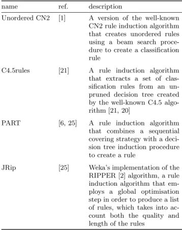
Table 2: The 4 rule induction algorithms used in the second set of experiments in addition to the c Ant-MinerPB and Unordered cAnt-MinerPB algorithms.

name ref. description

Unordered CN2 [1] A version of the well-known

CN2 rule induction algorithm that creates unordered rules using a beam search proce-dure to create a classification rule

C4.5rules [21] A rule induction algorithm

that extracts a set of clas-sification rules from an un-pruned decision tree created by the well-known C4.5 algo-rithm [21, 20]

PART [6, 25] A rule induction algorithm

that combines a sequential covering strategy with a deci-sion tree induction procedure to create a rule

JRip [25] Weka’s implementation of the

RIPPER [2] algorithm, a rule induction algorithm that em-ploys a global optimisation step in order to produce a list of rules, which takes into ac-count both the quality and length of the rules

4.2 Comparisons with state-of-the-art

classi-fication algorithms

The computational experiments comparing the proposed Unordered cAnt-MinerPB

2

algorithm against state-of-the-art rule induction algorithms were carried out using a set of 18 publicly available datasets from the UCI Machine Learn-ing repository [5]—a summary of the datasets used in the experiments is presented in Table 1. The second and third columns give the number of nominal and continuous at-tributes, respectively, for each dataset. The other column names are self-explained.

We have selected 4 rule induction algorithms, in addition to the cAnt-MinerPB

3

and Unordered cAnt-MinerPB algo-rithms. The details of the selected algorithms are given in Table 2. All algorithms were used with the default param-eter values proposed by their corresponding authors—both

cAnt-MinerPBand UnorderedcAnt-MinerPBwere used with the same parameter values from the first set of experiments (see Subsection 4.1). We used 2 configurations for the Un-orderedcAnt-MinerPB: one using the rule selection conflict resolution strategy (denoted as U-cAMPB[S]) and one using 2

The source-code and binaries of the new Unordered

cAnt-MinerPB algorithm are available for download at http://sourceforge.net/projects/myra.

3

We used thecAnt-MinerPBalgorithm with the error-based list quality function, as suggested by [13].

(6)

Table 3: Average predictive accuracy (average [standard error]) in %, measured by tenfold cross-validation. The value of the most accurate algorithm for a given dataset is shown in boldface.

dataset U-cAM_PB[S] U-cAM_PB[A] Unordered CN2 C4.5rules PART JRip cAnt-Miner_PB

annealing 97.70 [0.13] 95.53 [0.23] 88.10 [0.84] 94.22 [0.62] 94.88 [0.98] 94.43 [0.81] 97.34 [0.11] balance-scale 77.82 [0.20] 88.85 [0.21] 79.34 [1.39] 74.87 [1.16] 77.12 [1.40] 72.95 [1.92] 76.26 [0.29] breast-l 74.02 [0.19] 73.59 [0.35] 73.44 [1.81] 68.56 [1.93] 68.94 [1.80] 69.26 [2.04] 75.27 [0.35] breast-tissue 65.91 [0.67] 67.58 [0.72] 63.35 [4.51] 66.16 [2.97] 64.36 [3.63] 60.18 [3.35] 64.16 [0.98] breast-w 95.20 [0.12] 95.02 [0.19] 93.15 [1.51] 94.18 [1.14] 94.19 [1.12] 93.66 [1.42] 94.34 [0.16] credit-a 84.93 [0.28] 85.68 [0.16] 82.93 [1.49] 85.53 [1.53] 83.33 [1.04] 86.52 [1.10] 86.10 [0.23] credit-g 72.84 [0.32] 71.08 [0.22] 74.60 [0.98] 71.60 [0.92] 70.60 [1.49] 72.20 [1.07] 73.67 [0.28] cylinder-bands 72.06 [0.42] 71.83 [0.41] 76.85 [2.05] 76.48 [2.56] 72.41 [2.23] 68.70 [2.33] 72.36 [0.35] dermatology 90.54 [0.32] 90.08 [0.44] 87.43 [1.60] 93.45 [1.22] 94.26 [1.17] 88.01 [2.25] 92.40 [0.40] glass 69.46 [0.81] 68.24 [0.81] 65.73 [3.97] 68.63 [1.70] 72.81 [3.42] 65.71 [3.74] 73.11 [0.61] heart-c 56.66 [0.50] 57.13 [0.52] 55.81 [2.27] 53.12 [1.92] 53.83 [1.33] 53.50 [1.52] 55.21 [0.41] heart-h 64.64 [0.45] 64.02 [0.33] 60.90 [1.20] 63.31 [1.40] 63.64 [1.58] 63.93 [1.29] 65.92 [0.35] ionosphere 89.44 [0.33] 89.85 [0.35] 91.73 [2.77] 90.85 [2.59] 90.59 [2.00] 87.45 [2.64] 89.95 [0.23] iris 94.33 [0.20] 93.87 [0.19] 92.66 [1.55] 95.32 [1.42] 93.33 [1.99] 96.00 [1.09] 93.13 [0.26] liver-disorders 69.78 [0.64] 69.49 [0.46] 66.37 [1.52] 64.90 [3.21] 62.70 [3.40] 66.34 [2.80] 66.71 [0.41] parkinsons 87.75 [0.45] 85.28 [0.62] 86.66 [1.38] 83.49 [2.23] 86.05 [2.47] 84.53 [2.55] 87.42 [0.50] pima 74.55 [0.30] 74.32 [0.15] 73.42 [1.13] 74.32 [1.73] 71.73 [1.71] 73.55 [1.63] 74.67 [0.20] wine 95.46 [0.30] 95.48 [0.32] 93.80 [1.54] 91.03 [2.05] 91.54 [1.52] 92.68 [2.09] 94.51 [0.31]

Table 4: Statistical test results of the algorithms’ average predictive accuracies according to the non-parametric Friedman test with the Hommel’s post-hoc test. Statistically significant differences at the

α= 0.5level are shown in boldface.

Algorithm Avg. Rank p-value Hommel

U-cAMPB[S] (control) 2.72 – – cAnt-MinerPB 2.89 0.8169 0.05 U-cAMPB[A] 3.28 0.4404 0.025 PART 4.55 0.0108 0.0166 Unordered CN2 4.55 0.0108 0.0125 C4.5rules 4.83 0.0034 0.0100 JRip 5.17 6.8E-4 0.0083

the rule aggregation conflict resolution strategy (denoted as U-cAMPB[A]).

Table 3 presents the results concerning the predictive ac-curacy, where the higher the value the better the algorithm performance in terms of accuracy, measured as the aver-age value obtained by an algorithm at the end of the ten-fold cross-validation procedure. In the case of stochastic al-gorithmscAnt-MinerPB and UnorderedcAnt-MinerPB, the average value is computed over 10 executions of the ten-fold cross-validation procedure (i.e., each algorithm is run 10×10 times for each dataset); the remaining algorithms

are deterministic and the average is computed over a single run of the tenfold cross-validation (i.e., each algorithm is run 1×10 times for each dataset). Table 4 presents the statis-tical test results according to the non-parametric Friedman test with the Hommel’s post-hoc test [3, 8]: the first column corresponds to the algorithm’s name, the second column cor-respond to the average rank—where the lower the rank the better the algorithm’s performance—obtained in the Fried-man test, the third column shows thep-value of the statis-tical test when the average rank is compared to the average rank of the algorithm with the best rank (the ‘control’ algo-rithm), and the fourth column corresponds to the Hommel’s critical value. A row is shown in boldface when there is a statistically significant difference at the 5% significance level between the average ranks of an algorithm and the control algorithm, determined by the fact that the p-value is lower than Hommel’s critical value—i.e., it corresponds to the case where the control algorithm is significantly better than the algorithm in that row.

The UnorderedcAnt-MinerPBusing the rule selection con-flict resolution strategy (denoted as U-cAMPB[S]) achieved the best average rank, outperforming state-of-the-art rule in-duction algorithms with statistically significant differences, namely PART, Unordered CN2, C4.5rules and JRip. The use of the rule selection conflict resolution strategy led to an improvement in predictive accuracy, as in our initial ex-periments (Subsection 4.1), although the differences are not statistically significant when compared to the use of the rule aggregation conflict resolution strategy. While there are no statistically significant differences betweencAnt-MinerPB and Unordered cAnt-MinerPB algorithms, the results ob-tained by the proposed Unordered cAnt-MinerPB are

(7)

pos-itive, overall: the discovery of unordered rules explicitly improves their interpretability (i.e., a particular rule has a modular meaning independent of the others rules), without sacrificing the predictive accuracy.

4.3 Interpretability of the discovered rules

In order to quantify the interpretability of the discov-ered rules, we propose a new measure, called prediction-explanation size. Before presenting the details of how this measure is calculated, it is worth discussing the problems with the commonly-used model size as a measure of com-prehensibility (or interpretability). The model size measure, usually determined by the number of rules and the size of rules present in the list/set of rules, ignores how the rules are used to make class predictions—e.g., if a single or mul-tiple rules are needed to classify an example. In addition, there is evidence showing that, in some applications, larger models were considered by users as more comprehensible than smaller ones, since they contained more informative attributes to the user [11, 10]. An empirical study tested the assumption that smaller models are more comprehensi-ble to users [9]. The findings of this study indicate that the comprehensibility of the model from a user perspective tends to increase in line with the size of the model. Additionally, the concept of ‘small’ or ‘large’ is subjective—e.g., in [22] it is reported that users found that a model with 41 rules was considered too large to be analysed by a user, while in [24] a user analysed 29,050 rules and identified a subset of 220 in-teresting rules. Therefore, the model size—either measured as the number of rules or the total number of attribute-conditions of the rules—is not an adequate indicator of the comprehensibility of a classification model.

We define the prediction-explanation size as the average number of attributes-conditions (terms) that are evaluated in the model in order to predict the class value of an ex-ample, where the average is computed over all examples being classified in the test set. The rationale behind the prediction-explanation size measure is that it provides an estimate of the number of attributes-conditions that a user has to analyse in order to interpret a model’s prediction and those attribute-conditions can be regarded as an ex-planation for the class prediction. In the case of the origi-nalcAnt-MinerPBalgorithm, which produces an ordered list of rules, the prediction-explanation size is calculated taking into account all rules that are evaluated in order to make a prediction. E.g., if there are 3 rules in the list, each com-posed by 3 attributes-conditions, and the second rule is used to make a prediction, the prediction-explanation size is the sum of the attributes-conditions of the first and second rules. While the first rule is not directly involved in the prediction, it is involved indirectly in the prediction, since the second rule is only evaluated if the first rule is not used (i.e., its attribute-conditions evaluate to false).

In the case of the Unordered cAnt-MinerPB algorithm, which produces an (unordered) set of rules, the prediction-explanation size depends on the conflict resolution strat-egy used. When the rule selection stratstrat-egy is used, only one rule is responsible for the prediction and therefore, the prediction-explanation size is the number of attribute-condi-tions of the rule. When the rule aggregation strategy is used, the prediction-explanation size is the sum of the attribute-conditions of the rules that cover the example, since all rules that cover the example contribute to the final prediction. It

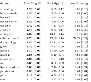
Table 5: Average number of attribute-conditions (terms) involved in the classification of an example. The value of the algorithm with the lowest average for a given dataset is shown in boldface.

dataset U-cAM_PB[S] U-cAM_PB[A] cAnt-Miner_PB

annealing 2.28 [0.01] 5.65 [0.12] 8.00 [0.19] balance-scale 1.40 [0.01] 5.09 [0.06] 4.94 [0.06] breast-l 2.74 [0.05] 8.94 [0.12] 5.30 [0.34] breast-tissue 1.47 [0.01] 4.35 [0.06] 3.89 [0.06] breast-w 1.40 [0.01] 7.11 [0.08] 3.91 [0.14] credit-a 2.76 [0.06] 8.73 [0.17] 6.61 [0.39] credit-g 2.83 [0.05] 13.11 [0.15] 15.77 [0.36] cylinder-bands 2.78 [0.04] 12.38 [0.15] 27.71 [0.77] dermatology 3.46 [0.06] 14.11 [0.29] 14.91 [0.33] glass 2.39 [0.04] 5.72 [0.06] 6.93 [0.15] heart-c 3.12 [0.03] 14.50 [0.26] 11.89 [0.38] heart-h 2.88 [0.05] 8.12 [0.04] 5.81 [0.21] ionosphere 3.05 [0.03] 7.07 [0.10] 6.51 [0.14] iris 1.38 [0.01] 3.09 [0.09] 2.80 [0.04] liver-disorders 2.38 [0.02] 7.48 [0.06] 12.44 [0.27] parkinsons 1.53 [0.03] 4.78 [0.06] 3.64 [0.07] pima 2.19 [0.03] 6.38 [0.03] 5.24 [0.07] wine 1.13 [0.01] 3.27 [0.05] 3.04 [0.03]

should be noted that in the UnorderedcAnt-MinerPB algo-rithm, each rule does have a modular meaning independent of the others, regardless of the conflict resolution strategy used, since the order of the rules is not important.

Table 5 presents the results (average[standard error]) con-cerning the prediction-explanation size of the models dis-covered by thecAnt-MinerPBand UnorderedcAnt-MinerPB algorithms, the lower the value the better the algorithm performance. The advantage of unordered rules combined with the rule selection strategy (denoted as U-cAMPB [S]) are clear: in all the datasets, it has the lowest number of attribute-conditions involved in the classification of an ex-ample. Overall, these results are positive: we were able to improve the interpretablity of the rules (measured as the prediction-explanation size) by discovering unordered rules, with no negative impact on the predictive accuracy. The Unordered cAnt-MinerPB with the rule selection strategy was the algorithm that achieved the best rank in terms of predictive accuracy and the best value for the prediction-explanation size measure.

5. CONCLUSION

In this paper we have proposed an extension to thec Ant-MinerPB in order to discover unordered rules, called Un-orderedcAnt-MinerPB. The main motivation is to improve the interpretation of individual rules. In an ordered list of rules, the effect (meaning) of a rule depends on all previ-ous rules in the list, since a rule is only used if all previprevi-ous rules do not cover the example. On the other hand, in an unordered set of rules, an example is shown to all rules and, depending on the conflict resolution strategy, a single rule is used to make a prediction.

We compared the proposed UnorderedcAnt-MinerPB al-gorithm against state-of-the-art rule induction alal-gorithms

(8)

in 18 publicly available datasets. The Unordered c Ant-MinerPB algorithm achieved the best results in terms of predictive accuracy, outperforming state-of-the-art rule in-duction algorithms with statistically significant differences. We also proposed a new measure to characterise the inter-pretability of the discovered rules. Our results show that the predictions made by an unordered set of rules are poten-tially easier to be interpreted by a user, due to the nature of unordered rules (i.e., each rule has a modular meaning inde-pendent of the others) and there are less attribute-conditions involved in the predictions.

While in this work we have evaluated different rule quality and list quality functions, the UnorderedcAnt-MinerPB al-gorithm’s more specific parameters were not optimised, since we focused in comparing the differences between ordered and unordered rules. It might be possible to further improve the algorithm evaluating different parameter settings. The eval-uation of different conflict resolution strategies can also lead to improvements to the predictive accuracy of the discovered rules.

6. REFERENCES

[1] P. Clark and R. Boswell. Rule Induction with CN2: Some Recent Improvements. InMachine Learning – Proceedings of the Fifth European Conference (EWSL-91), pages 151–163, 1991.

[2] W. Cohen. Fast effective rule induction. InProceedings of the 12th International Conference on Machine Learning, pages 115ˆa ˘A¸S–123. Morgan Kaufmann, 1995.

[3] J. Demˇsar. Statistical Comparisons of Classifiers over Multiple Data Sets.Journal of Machine Learning Research, 7:1–30, 2006.

[4] U. Fayyad, G. Piatetsky-Shapiro, and P. Smith. From data mining to knowledge discovery: an overview. In U. Fayyad, G. Piatetsky-Shapiro, P. Smith, and R. Uthurusamy, editors,Advances in Knowledge Discovery & Data Mining, pages 1–34. MIT Press, 1996.

[5] A. Frank and A. Asuncion. UCI machine learning repository, 2010.

[6] E. Frank and I. Witten. Generating Accurate Rule Sets Without Global Optimization. In J. Shavlik, editor,Proceedings of the Fifteenth International Conference on Machine Learning, pages 144–151. Morgan Kaufmann, 1998.

[7] A. Freitas, R. Parpinelli, and H. Lopes. Ant colony algorithms for data classification. InEncyclopedia of Information Science and Technology, volume 1, pages 154–159. Information Science Reference, 2nd edition, 2008.

[8] S. Garc´ıa and F. Herrera. An Extension on “Statistical Comparisons of Classifiers over Multiple Data Sets” for all Pairwise Comparisons.Journal of Machine Learning Research, 9:2677–2694, 2008.

[9] J. Huysmans, K. Dejaeger, C. Mues, J. Vanthienen, and B. Baesens. An empirical evaluation of the comprehensibility of decision table, tree and rule based predictive models.Decision Support Systems, 51:141–154, 2011.

[10] H. A. N. Lavesson. User-oriented assessment of classification model understandability. InProceedings

of the 11th Scandinavian Conference on Artificial Intelligence (SCAI), pages 11–19. IOS Press, 2011. [11] N. Lavrac. Selected techniques for data mining in

medicine.Artificial Intelligence in Medicine, 16:3–23, 1999.

[12] D. Martens, B. Baesens, and T. Fawcett. Editorial survey: swarm intelligence for data mining.Machine Learning, 82(1):1–42, 2011.

[13] M. Medland, F. Otero, and A. Freitas. Improving the

cAnt-MinerPBClassification Algorithm. In M. Dorigo, M. Birattari, C. Blum, A. L. Christensen, A. P. Engelbrecht, R. Groß, and T. St¨utzle, editors,Swarm Intelligence, volume 7461 ofLecture Notes in

Computer Science, pages 73–84. Springer Berlin Heidelberg, 2012.

[14] C. Nalini and P. Balasubramanie. Discovering Unordered Rule Sets for Mixed Variables Using an Ant-Miner Algorithm. Data Science Journal, 7:76–87, 2008.

[15] J. Olmo, J. Romero, and S. Ventura. Using Ant Programming Guided by Grammar for Building Rule-Based Classifiers. IEEE Transactions on Systems, Man, and Cybernetics, Part B: Cybernetics, 41:1585–1599, 2011.

[16] J. Olmo, J. Romero, and S. Ventura. Classification rule mining using ant programming guided by

grammar with multiple pareto fronts.Soft Computing, 16:2143–2163, 2012.

[17] F. Otero, A. Freitas, and C. Johnson. A New Sequential Covering Strategy for Inducing Classification Rules With Ant Colony Algorithms. IEEE Transactions on Evolutionary Computation, 17(1):64–76, 2013.

[18] R. Parpinelli, H. Lopes, and A. Freitas. Data mining with an ant colony optimization algorithm.IEEE Transactions on Evolutionary Computation, 6(4):321–332, 2002.

[19] G. Piatetsky-Shapiro and W. Frawley.Knowledge Discovery in Databases. AAAI Press, 1991.

[20] J. Quinlan. Improved Use of Continuous Attributes in C4.5.Artificial Intelligence Research, 7:77–90, 1996. [21] J. R. Quinlan.C4.5: programs for machine learning.

Morgan Kaufmann Publishers Inc., San Francisco, CA, USA, 1993.

[22] M. Schwabacher and P. Langley. Discovering communicable scientific knowledge from spatio-temporal data. InProceedings of 18th International Conference on Machine Learning (ICML-2001), pages 489–496. Morgan Kaufmann, 2001.

[23] J. Smaldon and A. Freitas. A new version of the ant-miner algorithm discovering unordered rule sets. InProc. Genetic and Evolutionary Computation Conference (GECCO 2006), pages 43–50, 2006. [24] S. Tsumoto. Clinical knowledge discovery in hospital

information systems: two case studies. InProceedings of European Conference on Principles and Practice of Knowledge Discovery and Data Mining (PKDD-2000), pages 652–656. Springer, 2000.

[25] H. Witten and E. Frank.Data Mining: Practical Machine Learning Tools and Techniques. Morgan Kaufmann, 2nd edition, 2005.

Improving the interpretability of classification rules discovered by an ant colony algorithm.