Optimization of Image Features using Artificial Bee
Colony Algorithm and Multi-layered Perceptron
Neural Network for Texture Classification
Muhammad Suzuri Hitam, Fthi M. Albkosh and Wan Nural Jawahir HjWan Yussof
School of Informatics and Applied Mathematics,
Universiti Malaysia Terengganu, 21030 Kuala Nerus, Terengganu, Malaysia. [email protected]
Abstract—One of the fundamental issues in texture classification is the suitable selection combination of input parameters for the classifier. Most researchers used trial and observation approach in selecting the suitable combination of input parameters. Thus it leads to tedious and time consuming experimentation. This paper presents an automated method for the selection of a suitable combination of input parameters for gray level texture image classification. The Artificial Bee Colony (ABC) algorithm is used to automatically select a suitable combination of angle and distance value setting in the Gray Level Co-occurrence (GLCM) matrix feature extraction method. With this setting, 13 Haralick texture features were fed into Multi-layer Perceptron Neural Network classifier. To test the performance of the proposed method, a University of Maryland, College Park texture image database (UMD Database)is employed. The texture classification results show that the proposed method could provide an automated approach for finding the best input parameters combination setting for GLCM which leads to the best classification accuracy performance of binary texture image classification.
Index Terms—Artificial Bee Colony Algorithm; Multi-layer Perceptron; Neural Network; Texture Classification.
I. INTRODUCTION
Texture images can be represented by either uniform or non-uniform patterns which repeat over an image region. Texture images often suffer wide variations in perceptual appearance due to variation in coarseness, contrast, uniformity. Due to its complexity, up to this moment,researchers are still looking for the best feature extraction method that could represent texture patterns. Therefore, finding a feature extraction method that can efficiently represent image texture is a fundamental problem in texture classification. At present, there are various texture classification methods exist, and they can be categorized as statistical approaches, signal-processing based approaches and structural approaches [1].
Over the last few decades, researchers have proposed many feature extraction methods including Gray Level Co-occurrence Matrix (GLCM) [2], Gray Level Run Lengths (GLRL) matrices [3], Wavelet Transforms [4], Gabor Filters [5], etc. A major problem in the texture feature extraction process is that there is no consensus in the literature about which feature extraction method that is the best to represent the texture patterns. The primary reason for this challenge is that texture images that appear in nature are very complex to be able for representation by a single universal method. Therefore, to date, no single feature extraction method can completely describe and represent all texture patterns fully [6,
7].
Among the statisticalbased methods that are very popular in representing texture, patterns are the GLCM [2]. Gui et al. [8] and Celik and Tjahjadi [9] claimed that this method is a very powerful texture descriptor used in texture image analysis and GLCM has been successfully applied in many types of research works. The main contributing factors that make GLCM method is very powerful is its concept of co-occurrence of texture patterns that rely on second ordered statistical analysis. However, the limitation of GLCM is, it is sensitive to two main parameters; angle and distance. The practitioners need to carry out extensive experimentations to determine the suitable combination of distance and angle predefined in GLCM method [10, 11] before it could be used in texture analysis or texture classification. Therefore, an automated mechanism for finding the optimal combination of suitable GLCM parameters will not only save practitioner’s time, but it would lead to best texture classification results.
This paper introduces a new automated approach for binary texture classification where the Artificial Bee Colony (ABC) algorithm [17] is employed to find the best combination of angle and distance in GLCM method. The rest of this paper is organized as follows; Section II presents the related work; Section III describes the basic theory of feature extraction of GLCM, ABC algorithm, and Multi-layer Perceptron Classifier. Section IV explains the framework of the proposed research methodology. Section V describes the experimental setup of the proposed research; in section VI the experimental results are presented and discussed; finally, Section VII concludes this work with possible future extension work.
II. RELATED WORKS
Texture classification aims to assign texture labels to unknown textures according to training samples and classification rules. Two major issues that are critical for texture classification: feature extraction and classification algorithm.
GLCM have been widely used for various texture analysis applications for texture classification. Tou et al. [12] reported a study for wood recognition system which used GLCM as feature extraction method and Multi-layered Perceptron Neural Network (MLPNN) as a classifier. They manually selected four angles (i.e., at 0, 45, 90, 135) and at a fixed distance equal to 1. These manual experimentation results in exhaustive experimentations even though they only experimented 50 images from five different wood species;
i.e., 25 training and 25 testing image samples. They reported a low recognition rate of 72% and 60% accuracy, respectively. In [13], Tou et al. showed that using a combination of GLCM and Gabor filters could result in better classification accuracy as compared to using a single GLCM extracted features. They manually experimented various combination of features from GLCM and Gabor Filters.
Pramunendar et al. [14] used AutoMLP and SVM for the process of grading of the coconut wood quality. They used GLCM method to extract 21 texture features at various combination of distances (i.e., 1, 2, 3) and angles (i.e., 0, 45, 90, 135). They have to manually run the trial and observation experiment to find the best combination of features that produced the best wood grading quality. The performance of AutoMLP classifier produced the best result, i.e., at the accuracy of 78.8% using the angle at 90 and distance at 3, which is slightly better than using Support Vector Machine (SVM) that produced 77.1% accuracy at the angle of 135 and distance of 3. Similarly, Othmen et al. [15] manually experimented the combination of wavelet and co-occurrence matrices features for texture classification. Similarly, Pathak and Barooah [10] also used GLCM for feature extraction in various angle with specified distance selected manually. From this literature, it can be concluded that the choice of angle and distance in GLCM parameters are critical for the performance of classification accuracy and works have been done by using a manual approach that leads to extensive experimentation.
Nowadays, with the availability of wide verity of optimization methods, there have been a few efforts by researchers to use them for selecting the best combination of input parameters for texture classification. Hasan et al. [16] proposed an application of Binary Particle Swarm Optimization (BPSO) algorithm in automatic classification of wood species. The texture features of the images are extracted using GLCM method. In their work, the BPSO algorithm is used to optimize the GLCM parameters: angle, distance and the number of gray-level and k-NN is used as a texture classifier. The results of their work showed that the BPSO could lessen the number of texture features used but the classification accuracy is only 68.4%.
Artificial Bee Colony Algorithm (ABC) is a swarm intelligence algorithm suggested by Karaboga in 2005 [17]. This global optimization algorithm which mimics the foraging behavior of honeybees is a flexible algorithm with few control parameters [18]. It has been employed to solve many different optimization problems in various areas.
Zhang et al. [19] proposed a hybrid method based on the feed-forward neural network used a modified ABC algorithm to select the weights and biases of the network for binary classification of MR brain image. Sathya and Geetha [20] presents an intelligent computer assisted mass classification method for breast DCE-MR images. It uses the ABC algorithm to optimize the neural network for classification of benign and malignant breast DCE-MR images. The network was found to yield good diagnostic accuracy. Uzer et al. [21] used ABC algorithm for the optimization of feature selection process in the classification of liver and diabetes database, where there are some redundant and low-distinctive features. These features are critical factor affecting the success of the classifier and the system processing time. SVM is used as a classifier. Classification accuracy of the proposed system reached 94.92%, 74.81%, and 79.29% for hepatitis dataset, liver disorders dataset and diabetes dataset, respectively.
Shanthi and Bhaskaran [22] suggested using ABC algorithm as a feature selection technique to select the predominant feature set in the classification of breast lesion in mammogram images. The performance of the proposed method was compared with that of GA and particle swarm optimization. It has been reported that out of 84 features, GA and particle swarm optimization select 50 and 56 features, respectively, while the proposed method selects only 42 features for the images used in the experiments and maintains the high accuracy of classification.
Based on these previous studies, the GLCM methods have been popularly used in many texture classification application. The main issues are its limitation in selecting the suitable combination of parameters, i.e. angle and distance. In this paper, we proposed a method to use ABC algorithm for automated selection of a suitable combination of angle and distance in GLCM and employed MLPNN as a classifier.
III. THEORY
A. Gray Level Co-occurrence Matrix (GLCM)
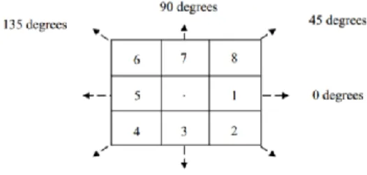
The GLCM is a very popular and powerful texture descriptor used in texture image analysis [9]. In this method, co-occurrence matrix was extracted based on second order statistics of the gray level values of pixels with given distance and angle [2]. The matrix is formed by computing how often a pixel with the gray-level intensity value, i occurs in a particular spatial relationship to a pixel with the value, j. Figure 1 illustrates the co-occurrence matrices for the direction in horizontal (θ = 0), vertical direction (θ = 90) and both diagonal directions (θ = 45; 135). Therefore, matrices providing different information could be obtained by modifying the spatial relationship (different orientation or distance between pixels).
Figure 1: The concept of angle in GLCM
Mathematically this relationship can be represented as: 𝑃 (𝑖, 𝑗, 𝑑, 0°) = #{((𝑘, 𝑙), (𝑚, 𝑛)) ∈ 𝑁 𝑤ℎ𝑒𝑟𝑒 ( 𝑘 − 𝑚 = 0, |𝑙 − 𝑛| = 𝑑 ), 𝐼(𝑘, 𝑙) = 𝑖, 𝐼(𝑚, 𝑛) = 𝑗} (1) 𝑃 (𝑖, 𝑗, 𝑑, 45°) = #{((𝑘, 𝑙), (𝑚, 𝑛)) ∈ 𝑁 𝑤ℎ𝑒𝑟𝑒 ( 𝑘 − 𝑚 = 𝑑, 𝑙 − 𝑛 = − 𝑑 )𝑜𝑟 ( 𝑘 − 𝑚 = −𝑑, 𝑙 − 𝑛 = 𝑑 ), 𝐼(𝑘, 𝑙) = 𝑖, 𝐼(𝑚, 𝑛) = 𝑗} (2) 𝑃 (𝑖, 𝑗, 𝑑, 90°) = #{((𝑘, 𝑙), (𝑚, 𝑛)) ∈ 𝑁 𝑤ℎ𝑒𝑟𝑒 (|𝑘 − 𝑚| = 𝑑, 𝑙 − 𝑛 = 0 ), 𝐼(𝑘, 𝑙) = 𝑖, 𝐼(𝑚, 𝑛) = 𝑗} (3) 𝑃 (𝑖, 𝑗, 𝑑, 135°) = #{((𝑘, 𝑙), (𝑚, 𝑛)) ∈ 𝑁 𝑤ℎ𝑒𝑟𝑒 ( 𝑘 − 𝑚 = 𝑑, 𝑙 − 𝑛 = 𝑑 )𝑜𝑟 ( 𝑘 − 𝑚 = −𝑑, 𝑙 − 𝑛 = − 𝑑 ), 𝐼(𝑘, 𝑙) = 𝑖, 𝐼(𝑚, 𝑛) = 𝑗} (4)
where i and j are the horizontal row and vertical column in the image, d is the distance from the measured pixel in an image, # represents the number of elements in the set, and k,
l, m, n ∈ N.
Once the GLCM is computed, then texture feature descriptors are extracted from these matrices. Haralick’s texture features are perhaps the most popular statistical features to represent the texture image. Among these features are an angular second moment, contrast, correlation, the sum of squares, inverse difference moment, sum average, sum variance, sum entropy, entropy, difference variance, difference entropy, and two information measures of correlation.
B. Multi-Layer Perceptron Neural Network Classifier Multi-layer Perceptron Neural Network (MLPNN) [23] is perhaps the most popular neural network that has been used a neural network classifier. The Haralick features extracted from the GLCM were feed into MLPNN to classify the selected image textures. There are a variety of training algorithms been employed, and MLPNN has to be tuned for finding the best network configuration. In this paper, we are experimenting these settings manually in finding the optimal MLPNN setting for best classification results.
C. Optimization Algorithm
The ABC algorithm is a swarm based intelligent optimization algorithm that is inspired by honey bee foraging. It uses a concept of a population of artificial bees in its initialization. Their positions are considered as foods positions and modified with the time by finding out some places with high nectars [24]. The location of a food source represents a possible solution to the considered optimization problem, and the nectar amount of the food source corresponds to the quality or fitness of the associated solution. The number of the employed bees or onlooker bees is identical to the number of solutions in the population.
In ABC system, ABC algorithm generates randomly distributes a predefined number of initial population, (position of the food sources). After initialization, the population of the positions (solutions) is subjected to the frequent cycles until maximum iteration number of the search process of the employed bees, onlooker bees, and scout bees. An employed bee creates an adjustment on the solution in its memory depending on the local information. It tests the nectar amount (fitness value) of the new food source (new solution). If the nectar amount of the new food source is higher than that of the previous one, the bee memorizes the new position and forgets the old one. Otherwise, it keeps the location of the old food source in its memory.
When all the employed bees finish the search process, they share the nectar information of the food sources and their location information with the onlooker bees in the dance area. An onlooker bee assesses the nectar information obtained from all the employed bees and selects a food source with a probability related to its nectar amount. Like in the case of an employed bee, the onlooker bee creates a modification on location in its memory and examines the nectar amount of the candidate source. If its nectar amount is higher than that of the preceding one, the onlooker bee memorizes the new location and forgets the old one. Generally, in the ABC algorithm, the stopping criteria of an optimization algorithm is based on the maximum number of iterations.
IV. THE PROPOSED METHODOLOGY
A. Framework
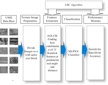
The proposed method attempts to optimize the given input through analyzed data set and eliminates the unnecessary calculation to increase the accuracy of the classification process. Figure 2 shows the framework of the proposed research method. It consists of four stages; texture image preparation, feature extraction, classification and performance measure. The first stage which is the texture image preparation is used to prepare input image for feature extraction. Before the texture image classification can take place, texture images were preprocessed in the texture image preparation stage. In the feature extraction stage, it calculates 13 Haralick texture features with different angles and distances. These features were later fed into MLPNN classifier and calculate the classification performances at each parameter combination. The ABC algorithm will choose the right combination of angle and distance in the GLCM parameters based on the best classifier performance. We named this act of parameter selection optimization algorithm as AGLCM in this paper.
Figure 2: The Proposed research framework
B. Implementation ABC to Optimize GLCM Parameters The GLCM method considers two main parameters related to neighboring points of pixel values which are distance and angle, normally selected manually by the user. To find the best combination of these parameter setting, we consider all angles and at four possible distances. The overall AGLCM algorithm is as depicted in Figure 3.
Step 1. Step 2. Step 3. Step 4. Step 5. Step 6. Step 7.
Randomly initialize food sources. (Initial population parameters for the ABC algorithm from different angles and distances of GLCM)
Calculate the nectar amount (accuracy) of the selected initial food sources.
Employed phase:
Set the iteration counter to 1.
Determine other possible positions of food sources for employed bees (i.e., new values of GLCM parameters). Calculate the nectar amount (accuracy) corresponding to the new food sources positions of the employed bees. Compare the fitness by new values with the fitness of the previous one to obtain the best fitness value.
If not all onlooker bees are distributed to food sources, update the new position for the onlooker bees and return to Step 4.
Step 8. Step 9. Step 10. Step 11.
Onlooker phase:
Calculate the nectar amount (accuracy) corresponding to the new food source position of the onlooker bees. Compare the fitness by new values with the fitness of the employed one to obtain the best fitness value.
Update the best food source position corresponding to fitness values.
If the maximum number of iterations is not reached, go to Step 4.
Figure 3: The AGLCM algorithm
C. Performance Measures
In this paper, the binary classification performances are measured using sensitivity, specificity and accuracy performance indicator [25].
1) Sensitivity (Sen)
Sen measures the proportions of correct classification (true positive rate) from the given data and can be expressed as follows:
Sen = True Positive
True Positive + False Negative (5)
2) Specificity (Spe)
The Spe is the proportions of incorrect classification, which is incorrectly classified. Spe can define as follows:
Spe = True Negative
(False Positive + True Negative) (6)
3) Accuracy (Acc)
Acc is the global representation of classifier performance and can be defined as follows:
Acc= (True Positive + True Negative)
(True Positive + False Positive+ False Negative + True Negative) (7) V. EXPERIMENTAL SETUP
In this paper, we have used the University of Maryland, College Park texture image database (UMD Database) as a texture image benchmark database.
A. UMD Image database
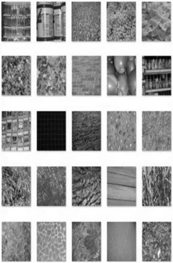
UMD image database consists of 25 image texture classes with 40 samples with a resolution of 1280*960 pixels. It contains significant viewpoint changes, scale differences with uncontrolled illumination condition. The dataset contains high intra-class variability and similarity between texture classes making the dataset a challenging problem for classification. The textures of this dataset are non-traditional, including images of fruits, various plants, floor textures, shelves of bottles and buckets. Figure 4 shows a sample texture image per class [26].
In this paper, we make some image preprocessing on the original UMD database to get a sufficient number of samples with different diversity. Firstly, we segment the original textures sample with size 128*128. Thus, we obtained a total of 2800 textures per each sample, and the smaller remaining portion of the images was discarded. Secondly, we randomly select a collection of 500 image textures from each 2800 samples. Thirdly, 35 binary textures grouping were formed, where each group contains 1000 texture images, i.e., 500 texture images from different samples. These images were later randomly selected 80% for the training set and 20% for
testing set.
Figure 4: Samples of UMD data set
B. Optimal GLCM Parameters
GLCM considers two parameters related to neighboring points which are distance and angle. In this work, we used ABC algorithm to find the best possible combination of four different angles with four different distances as shown in Table 1.
C. MLPNN
In this paper, the MLPNN with a single hidden layer of 60 neurons is used. The hyperbolic tangent activation function is utilized in the hidden layer, and linear function activation function is employed in the output layer. To increase the reliability and generality of the results, we choose 5-fold cross validation process.
Table 1
All parameters used in texture classification Angle 0° with four distances Angle 45° with four distances Angle 90° with four distances Angle 135°with four distances 0 45 90 135 1 2 3 4 1 2 3 4 1 2 3 4 1 2 3 4
VI. RESULTS AND DISCUSSION
The experiment was carried out using 25 samples for UMD dataset. Table 2 shows the performance of the classification results of all the 35 binary group classification test cases.
Table 2
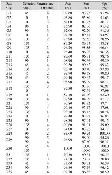
The results of texture classification with different combination of parameters.
Data Base
Selected Parameters Acc (%) Sen (%) Spe (%) Angle Distance G1 45 4 92.60 93.23 91.94 G2 0 1 93.80 95.80 91.63 G3 0 3 87.00 87.25 86.72 G4 90 1 86.90 82.36 91.42 G5 90 3 92.00 92.70 91.36 G6 0 1 92.30 89.47 94.97 G7 135 2 75.90 72.63 78.96 G8 135 4 89.20 89.94 88.38 G9 135 3 96.20 95.85 96.54 G10 0 4 96.40 96.38 96.35 G11 135 2 97.60 96.31 98.76 G12 90 1 98.90 98.36 99.39 G13 45 4 99.50 99.62 99.42 G14 135 3 98.70 99.40 97.98 G15 45 2 99.70 99.58 99.80 G16 45 3 99.40 99.62 99.17 G17 0 4 98.90 98.99 98.77 G18 135 3 97.30 97.86 96.91 0 4 97.39 97.09 G19 0 1 87.10 81.40 92.80 G20 135 4 82.90 84.39 81.17 G21 135 4 90.80 93.92 87.74 G22 90 4 90.10 93.17 87.08 G23 135 1 98.20 98.15 98.24 G24 0 3 97.40 97.82 96.94 G25 90 1 98.30 97.44 99.15 G26 135 4 90.60 91.91 89.09 G27 0 2 84.00 83.92 84.17 G28 90 2 99.60 99.24 100.00 G29 90 90 3 4 96.90 98.00 97.60 95.86 96.21 G30 45 4 100.0 100.0 100.0 135 4 100.0 100.0 G31 135 1 90.50 90.54 90.55 G32 135 3 74.50 78.07 70.88 G33 45 4 97.60 98.81 96.39 G34 90 3 96.80 97.16 96.42 G35 45 4 97.70 96.85 98.59
As can be observed from table 2, different combination of parameter value leads to different performance accuracy. For example, Group 30 give the best results out of all texture groups where it produces 100% accuracy with 100% specificity and sensitivity. From all the experiment, only two image groups provide less than 82% accuracy, i.e., image from Group 7 and Group 32 where its accuracy is 75.9% and 74.5%, respectively. In these texture groups, the texture patterns consist of very similar looking texture image. The texture patterns from both groups are perceptually very close from each other. Thus, the classification results are lower as compared from other texture groups. Overall classification performances are considered good or excellent because almost all classification group case studies provide more than 82% accuracy with almost similar sensitivity and specificity trends. The classification performances differ from one group to the other because the characteristics of the texture images differ with different image quality as well as texture patterns. Close up classification results on texture Group 18 is shown in Figure 5. It should be noted that sometimes the algorithm produces same classification accuracy performance. For example, the combination of two parameter values which are (135, 3) and (0, 4) produces 97.3% classification accuracy. As can be seen in Table 2, similar results were produced for Group 29 and Group 30. Figure 6 and Figure 7 show the results of AGLCM algorithm produced the best classification accuracy at an angle equal to zero degrees and a distance
equal to 1 for texture Group 2 and Group 6, respectively.
Figure 5: Classification testing performance graph for image Group 18
Figure 6: Testing accuracy performance for Group 2
Figure 7: Testing accuracy performance for Group 6
Based on the sensitivity and specificity values for of 35 groups, Group 1 which contains Screws and Buckets, AGLCM algorithm selected angle 45 degree and at a distance equal to 4 produced the classification accuracy of 92.60% while the sensitivity and specificity of AGLCM were 93.23% and 91.94%, respectively. These results mean that the accuracy is increased in class one (Screws) images of the group and slightly decreased with the class two (Buckets) images. These patterns were changed from one group to the other in other group results indicating that the texture pattern varies across the UMD database.
VII. CONCLUSION
Classifying the texture classes is one of the recent research issues in the field of image processing. The classification accuracy can be improved if and only if both the feature extraction and classifier selection are proper. In this paper, it has been shown that the best classification performance could be obtained after a series of optimization on angles and distances parameters of GLCM method. Thus, selection of
94 94.5 95 95.5 96 96.5 97 97.5 (1 3 5 ,4 ) (1 3 5 ,1 ) (0 ,3 ) (4 5 ,3 ) (4 5 ,2 ) (1 3 5 ,3 ) (9 0 ,1 ) (0 ,1 ) (4 5 ,4 ) (0 ,4 ) (0 ,2 ) (9 0 ,2 ) (4 5 ,1 ) (1 3 5 ,2 ) (9 0 ,3 ) (9 0 ,4 ) A cc u ar cy ( %) GLCM Parameters 90 90.5 91 91.5 92 92.5 93 93.5 94 (90, 2) (0, 1) (45, 1) (135, 4) (135, 2) (135, 1) (0, 3) (0, 2) (45, 4) (90, 3) (90, 1) (45, 3) (135, 3) (0,4 ) (90, 4) (45, 2) A cc u ar cy ( % ) GLCM Parameters 80 82 84 86 88 90 92 94 (4 5 ,1 ) (4 5 ,3 ) (0 ,3 ) (4 5 ,2 ) (1 3 5 ,1 ) (1 3 5 ,3 ) (0 ,1 ) (9 0 ,3 ) (1 3 5 ,2 ) (9 0 ,4 ) (0 ,4 ) (9 0 ,2 ) (4 5 ,4 ) (9 0 ,1 ) (1 3 5 ,4 ) (0 ,2 ) A cc u ra cy ( %) GLCM Parameters
parameter has been carried out automatically to find the best combination of parameters in GLCM. In conclusion, this paper has contributed in selecting the best combination of GLCM parameters automatically in binary texture classification. Further work can be carried out in the future whereby the ABC algorithm may be used for automatic selection of features as well as classifier optimization.
REFERENCES
[1] M. Tuceryan and A. K. Jain, “Texture analysis,” in The Handbook of Pattern Recognition and Computer Vision, Second ed., vol. 2, C. H. Chen, L. F. Pau, and P. S. P. Wang, Eds., World Scientific Publishing Co., pp. 207-248, 1998.
[2] R. M. Haralick and K. Shanmugam, “Textural features for image classification,” IEEE Trans. on Systems, Man, and Cybernetics, vol. 3, no. 6, pp. 610-621, 1973.
[3] M. M. Galloway, “Texture analysis using gray level run lengths,”
Computer Graphics and Image Processing, vol. 4 ,no. 2, pp. 172-179, 1975.
[4] M. Unser, “Texture classification and segmentation using wavelet frames,” IEEE Trans. on Image Processing, vol. 4, no. 11, pp. 1549-1560, 1995.
[5] G. Daugman, “Uncertainty relation for resolution in space, spatial frequency, and orientation optimized by two-dimensional visual cortical filters,” Journal of Optical Society of America A., vol. 2, no. 7, pp. 1160-1169, 1985.
[6] M. A. García and D. Puig, “Supervised texture classification by integration of multiple texture methods and evaluation windows,” Image and Vision Computing, vol. 25, no. 7, pp. 1091-1106, 2007. [7] Y. Hu and C.-x. Zhao, “Unsupervised texture classification by
combining multi-scale features and k-means classifier,” in Chinese Conference on Pattern Recognition 2009, 2009, pp. 1-5.
[8] W. Gui, J. Liu, C. Yang, N. Chen, and X. Liao, “Color co-occurrence matrix based froth image texture extraction for mineral flotation,”
Minerals Engineering, vol. 46-47, pp. 60-67, 2013.
[9] T. Celik and T. Tjahjadi, “Multiscale texture classification using dual-tree complex wavelet transform,” Pattern Recognition Letters, vol. 30, no. 3, pp. 331-339, 2009.
[10] B. Pathak and D. Barooah, “Texture analysis based on the gray-level co-occurrence matrix considering possible orientations,” International Journal of Advanced Research in Electrical, Electronics and Instrumentation Engineering, vol. 2, no. 9, pp. 4206-4212, 2013. [11] J. Y. Tou, Y. H. Tay, and P. Y. Lau, “One-dimensional grey-level
co-occurrence matrices for texture classification,” in 2008 International Symposium on Information Technology, 2008, pp. 1-6.
[12] J. Y. Tou, P. Y. Lau, and Y. H. Tay, “Computer vision-based wood recognition system,” in Proc. of Int. Workshop on Advanced Image Technology, 2007.
[13] J. Y. Tou, K. K. Y. Khoo, Y. H. Tay, and P. Y. Lau, “Evaluation of Speed and accuracy for comparison of texture classification implementation on embedded platform,” in Int. Workshop on Advanced Image Technology, 2009.
[14] R. A. Pramunendar, C. Supriyanto, D. H. Novianto, I. N. Yuwono, G. F. Shidik, and P. N. Andono, “A classification method of coconut wood quality based on gray level co-occurrence matrices,” in 2013 IEEE International Conference on Robotics, Biomimetics, and Intelligent Computational Systems (ROBIONETICS), 2013, pp. 254-257. [15] M. B. Othmen, M. Sayadi, and F. Fnaiech, “Interest of the
multi-resolution analysis based on the co-occurrence matrix for texture classification,” in MELECON 2008-The 14th IEEE Mediterranean Electrotechnical Conference, 2008, pp. 852-856.
[16] A. F. Hasan, M. F. Ahmad, M. N. Ayob, S. A. A. Rais, N. H. Saad, A. Faiz, et al., “Application of binary particle swarm optimization in automatic classification of wood species using gray level co-occurrence matrix and k-nearest neighbor,” Int. Journal of Sci. Eng. Res, vol. 4, no. 5, pp. 50-55, 2013.
[17] D. Karaboga, “An idea based on honey bee swarm for numerical optimization,” Technical report-tr06, Erciyes University, Engineering Faculty, Computer Engineering Department, 2005.
[18] D. Karaboga and B. Basturk, “A powerful and efficient algorithm for numerical function optimization: artificail bee colony (ABC) algorithm”, Journal of Global Optimization, vol. 39, no. 3, pp.459-471, 2007.
[19] Y. Zhang, L. Wu, and S. Wang, “Magnetic resonance brain image classification by an improved artificial bee colony algorithm,”
Progress In Electromagnetics Research, vol. 116, pp. 65-79, 2011. [20] D. J. Sathya and K. Geetha, “Mass classification in breast DCE-MR
images using an artificial neural network trained via a bee colony optimization algorithm,” ScienceAsia, vol. 39, pp. 294-305, 2013. [21] M. S. Uzer, N. Yilmaz, and O. Inan, “Feature selection method based
on artificial bee colony algorithm and support vector machines for medical datasets classification,” The Scientific World Journal, vol. 2013, pp. 1-10, 2013.
[22] S. Shanthi and V. M. Bhaskaran, “Modified artificial bee colony based feature selection: a new method in the application of mammogram image classification,” Int. J. Sci. Eng. Technol. Res, vol. 3, no. 6, pp. 1664-1667, 2014.
[23] D. Kriesel, A brief Introduction on Neural Networks. 2007. [Online]. Available at http://www.dkriesel.com/_media/science/neuronalenetze-en-zeta2-2col-dkrieselcom.pdf
[24] S. Talatahari, H. Mohaggeg, K. Najafi, and A. Manafzadeh, “Solving parameter identification of nonlinear problems by artificial bee colony algorithm,” Mathematical Problems in Engineering, vol. 2014, pp. 1-6, 2014.
[25] R. Kohavi and F. Provost, “Glossary of terms,” Machine Learning, vol. 30, no. 2-3, pp. 271-274, 1998.
[26] S. Hossain and S. Serikawa, “Texture databases–a comprehensive survey,” Pattern Recognition Letters, vol. 34, no. 15, pp. 2007-2022, 2013.