Performance Envelopes of Adaptive Ensemble Data Stream Classifiers

(1)

Nova Southeastern University

NSUWorks

CEC Theses and Dissertations College of Engineering and Computing

2017

Performance Envelopes of Adaptive Ensemble

Data Stream Classifiers

Stefan Joe-Yen

Nova Southeastern University,[email protected]

This document is a product of extensive research conducted at the Nova Southeastern UniversityCollege of Engineering and Computing. For more information on research and degree programs at the NSU College of Engineering and Computing, please clickhere.

Follow this and additional works at:https://nsuworks.nova.edu/gscis_etd Part of theComputer Sciences Commons

Share Feedback About This Item

This Dissertation is brought to you by the College of Engineering and Computing at NSUWorks. It has been accepted for inclusion in CEC Theses and Dissertations by an authorized administrator of NSUWorks. For more information, please [email protected].

NSUWorks Citation

Stefan Joe-Yen. 2017.Performance Envelopes of Adaptive Ensemble Data Stream Classifiers.Doctoral dissertation. Nova Southeastern University. Retrieved from NSUWorks, College of Engineering and Computing. (1014)

(2)

Performance Envelopes of Adaptive Ensemble Data Stream Classifiers by

Stefan Joe-Yen

A dissertation submitted in partial fulfillment of the requirements for the degree of Doctor of Philosophy

in

Computer Information Systems College of Engineering and Computing

Nova Southeastern University 2017

(3)

(4)

An abstract of a Dissertation submitted to Nova Southeastern University in Partial Fulfillment of the Requirements for the degree of Doctor of Philosophy

Performance Envelopes of Adaptive Ensemble Data Stream Classifiers by

Stefan Joe-Yen Summer 2017

Abstract

This dissertation documents a study of the performance characteristics of algorithms de-signed to mitigate the effects of concept drift on online machine learning. Several super-vised binary classifiers were evaluated on their performance when applied to an input data stream with a non-stationary class distribution. The selected classifiers included ensembles that combine the contributions of their member algorithms to improve overall performance. These ensembles adapt to changing class definitions, known as “concept drift,” often present in real-world situations, by adjusting the relative contributions of their members.

Three stream classification algorithms and three adaptive ensemble algorithms were com-pared to determine the capabilities of each in terms of accuracy and throughput. For each run of the experiment, the percentage of correct classifications was measured using pre-quential analysis, a well-established methodology in the evaluation of streaming classifiers. Throughput was measured in classifications performed per second as timed by the CPU clock. Two main experimental variables were manipulated to investigate and compare the range of accuracy and throughput exhibited by each algorithm under various conditions. The number of attributes in the instances to be classified and the speed at which the definitions of labeled data drifted were varied across six total combinations of drift-speed and dimen-sionality.The implications of results are used to recommend improved methods for working with stream-based data sources.

The typical approach to counteract concept drift is to update the classification models with new data. In the stream paradigm, classifiers are continuously exposed to new data that may serve as representative examples of the current situation. However, updating the ensemble classifier in order to maintain or improve accuracy can be computationally costly and will negatively impact throughput. In a real-time system, this could lead to an unacceptable slow-down.

The results of this research showed that, among several algorithms for reducing the effect of concept drift, adaptive decision trees maintained the highest accuracy without slowing down with respect to the no-drift condition. Adaptive ensemble techniques were also able to maintain reasonable accuracy in the presence of drift without much change in the throughput. However, the overall throughput of the adaptive methods is low and may be unacceptable for extremely time-sensitive applications. The performance visualization methodology utilized in this study gives a clear and intuitive visual summary that allows system designers to evaluate candidate algorithms with respect to their performance needs.

(5)

Acknowledgements

A project of this scope, even when it is primarily the result of a single author’s vision and effort, involves the time and support of many people. I would like to thank the following individuals who have made a significant contribution to my work and life in Melbourne, FL during the course of this study over the past few years.

First, my gratitude to Sumitra Mukherjee, Ph.D., at Nova Southeastern University Col-lege of Engineering and Computing for supervising my work and providing advice and mo-tivation throughout the process. Also, many thanks to the rest of my committee: Francisco Mitropoulos, Ph.D., and Michael Lazlo, Ph.D. for their additional guidance and support.

Next, I would like to express my gratitude to Northrop Grumman Corporation, and my managers including Gary Ranshous, for providing a flexible place to work and partial funding for my graduate studies. I would like to give special recognition to the research advisors and colleagues there who have influenced my work in advanced analytics and data science including Monte Hancock, John Day, Michael Black, Chadwick Sessions, Charles Ethan Hayes, Guy Hoenig (who introduced me to NSU), Adrian Peter, Ph.D., Donald Steiner, Ph.D., Brock Bose, Ph.D., Matthew Welborn, Ph.D. and Veronica Bloom, Ph.D.

Over the past few years, I suffered from chronic back pain due to degeneration and injury to multiple spinal discs. Thus, I give many thanks to the folks at Suntree Internal Medicine, Deuk Spine Institute, and Florida Sports and Spinal Rehab especially Bharat Patel, M.D., Edwin Chan, M.D., Tanya Schrumpf, D.C., Kristina Fowler, D.P.T., Daniel Ferrier, C.C.A., and Sarah Steele, L.M.T. who helped me get through the health related challenges as I completed this work.

Finally, I give my deepest thanks to my family - my wife, Cameron, for patiently support-ing me, and my parents, Eugene and Kathleen, for initiatsupport-ing and supportsupport-ing my constant quest for knowledge.

(6)

List of Figures

1.1. Example of Performance Envelope Visualization 13 3.1. Experiment Framework Architecture 33

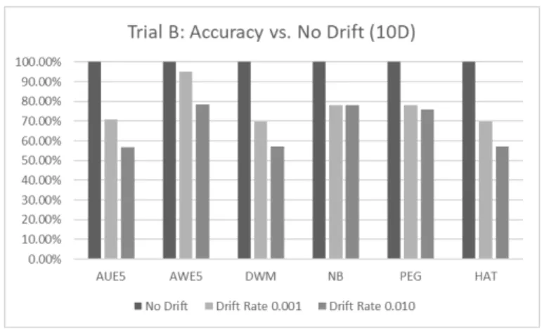
4.1. Trial B Accuracy on 10-Dimensional Instances 45 4.2. Trial B Accuracy on 50-Dimensional Instances 46

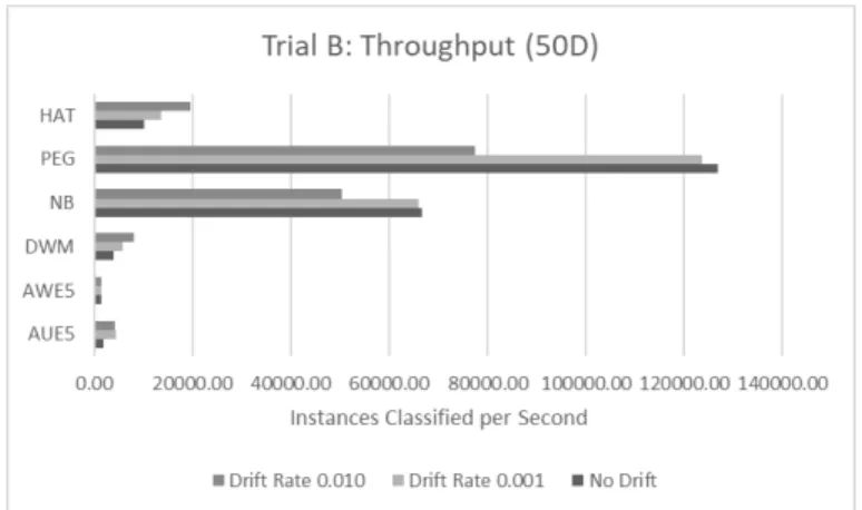
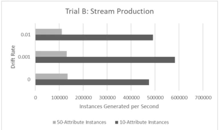
4.3. Trial B Relative Accuracy on 10-Dimensional Instances 47 4.4. Trial B Relative Accuracy on 50-Dimensional Instances 47 4.5. Trial B Throughput on 10-Dimensional Instances 48 4.6. Trial B Throughput on 50-Dimensional Instances 48 4.7. Trial B Stream Instance Generation Rate 49

4.8. Trial B Scaled Throughput on 10-Dimensional Instances 49 4.9. Trial B Scaled Throughput on 50-Dimensional Instances 50

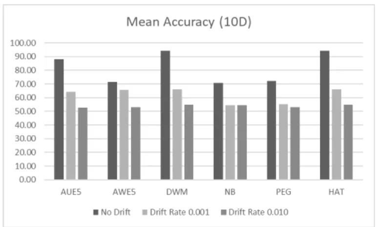
4.10. Coefficient of Variance (CV) of Accuracy across Experiment Trials 51 4.11. Mean Accuracy on 10-Dimensional Instances 52

4.12. Mean Accuracy on 50-Dimensional Instances 52

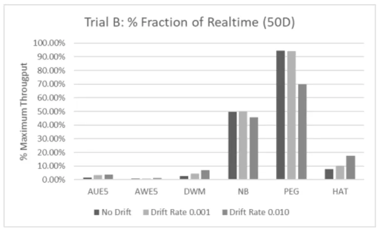
4.13. Mean Throughput as a Fraction of Real-Time Processing (10D) 53 4.14. Mean Throughput as a Fraction of Real-Time Processing (50D) 53 4.15. Mean Throughput of slower algorithms (10D) 54

4.16. Mean Throughput of slower algorithms (50D) 54 4.17. Accuracy vs. Throughput (10D) 55

4.18. Accuracy vs. Throughput (50D) 57 4.19. Pegasos SVM Time Series (10D) 58 4.20. Pegasos SVM Time Series (50D) 59 4.21. Naive Bayes Time Series (10D) 59 4.22. Naive Bayes Time Series (50D) 60

4.23. Hoeffding Adaptive Tree Time Series (10D) 60 4.24. Hoeffding Adaptive Tree Time Series (50D) 61 4.25. Dynamic Weighted Majority Time Series (10D) 61 4.26. Dynamic Weighted Majority Time Series (50D) 62 4.27. Accuracy Weighted Ensemble Time Series (10D) 62 4.28. Accuracy Weighted Ensemble Time Series (50D) 63 4.29. Accuracy Updated Ensemble Time Series (10D) 63 4.30. Accuracy Updated Ensemble Time Series (50D) 64 5.1. Welch PSD for DWM, 10 Dimensional input stream 66 5.2. Welch PSD for HAT, 50 Dimensional input stream 66

(9)

5.3. Correlations across classifiers, 50 Dimensional input stream at drift level (0.001) 67

C.1. Accuracy vs. Throughput Trade-off (10D) 85 C.2. Accuracy vs. Throughput Trade-off (50D) 86 C.3. Pegasos SVM Time Series (10D) 87

C.4. Pegasos SVM Time Series (50D) 88 C.5. Naive Bayes Time Series (10D) 89 C.6. Naive Bayes Time Series (50D) 90

C.7. Hoeffding Adaptive Tree Time Series (10D) 91 C.8. Hoeffding Adaptive Tree Time Series (50D) 92 C.9. Dynamic Weighted Majority Time Series (10D) 93 C.10. Dynamic Weighted Majority Time Series (50D) 94 C.11. Accuracy Weighted Ensemble Time Series (10D) 95 C.12. Accuracy Weighted Ensemble Time Series (50D) 96 C.13. Accuracy Updated Ensemble Time Series (10D) 97 C.14. Accuracy Updated Ensemble Time Series (50D) 98

(10)

Listings

B.1. TDEF script 71

B.2. StreamBenchmark script 77 B.3. StreamExample script 80

(11)

Chapter 1 Introduction

Background

This dissertation presents experimental research that evaluates algorithmic alternatives for a prevalent approach to analytics on streaming data. In particular, it addresses the problem of maintaining acceptable classification accuracy and throughput in a variety of supervised binary classifiers including ensemble approaches that continuously process input data as it arrives. The goal is to provide designers of decision support systems with theoretically grounded, and empirically supported basis for selecting among numerous alternatives avail-able for this class of algorithm.

The range of acceptable performance of an analytic system is defined by the nature of the intended application. Expected performance is subject to the constraints of specific characteristics of the data being processed and the available hardware. These constraints are often beyond the control of the system designer and end-user. However, due to the significant successes of a prolific research community, the machine learning approach has produced an embarrassment of riches when it comes to algorithms available for use. Only recently have any significant meta-analyses been performed to determine what the specific strengths and weaknesses of the various algorithms are in a systematic way.

In “Do we Need Hundreds of Classifiers to Solve Real World Classification Problems?” (Fern´andez-Delgado, Cernadas, Barro, & Amorim, 2014), a meta-analysis of 179 classifiers from 17 families of algorithms was conducted. This showed that decision-tree based learners

(12)

consistently performed exceptionally well. The study focused on evaluating non-streaming classifiers. With the continued rise of “Big Data,” The performance of data-stream classifiers is of growing importance. Thus we need a similar principled approach to comprehensively evaluating their performance characteristics. This study is a beginning toward that end.

This study focuses on a specific paradigm of machine learning algorithms and examines the behavior a small set of published algorithmic alternatives for classifying non-stationary streaming data. The results are intended to support principled guidelines for system archi-tects to produce high-performance systems.

One of the main challenges for machine learning on streams is the need for constant adaptation and re-training. Since the complete data set is not available in a static form, evidence for sorting inputs into target classes changes over time. Thus data used to train supervised classification algorithms may become obsolete, especially if the definition of the target classes is subsequently modified. Re-defining the classes, or other factors which change the underlying data distribution, adversely affects the performance of the classifier ensemble. If the models learned by the component classifiers no longer reflect the current situation, the accuracy of ensemble classification will suffer. Improving results depends on detecting when the classifiers are no longer performing acceptably and then using new data to update the model. However, the adaptive update or retraining of the classifiers incurs a computational cost. Thus, model updates should only occur when it would significantly benefit the accuracy of the results.

In the current paradigm of large-scale stream data mining, real-time analysis presents new challenges to machine learning techniques that were developed in the context of mining of static databases, also called “data-at-rest.” Stream based pattern recognition software operates in-line as the data arrives. The data is usually not stored and thus not available for re-processing by the algorithm. This type of data is commonly referred to as streaming data, also called “data-in-motion.” The measurable indicators of underlying patterns in the data may change over time. For large-scale computing, also known as “Big Data,” this poses new

(13)

challenges in data mining algorithm design and implementation. The rate of data production in information systems has already exceeded the available resources for storing such data (Bifet et al., 2010). Also, the relevance of the data collected in many domains expires rapidly. End users in domains such as defense and finance look to automated information processing systems to produce timely and accurate analyses of rapidly changing data sources to support their decisions. Therefore, solutions that adapt to changing circumstances to maintain the accuracy of their results while continuing to process data rapidly are highly desirable. The demand for real-time systems is only expected to increase moving forward.

This research examines open questions related to maintaining high data processing through-put in supervised stream classification while preserving accuracy. The following sections and chapters describe the motivation for the questions that were explored in this study. The context in which classifier performance was examined is described briefly below. Detailed definitions of the experimental variables are presented in the “Problem Statement” section. An experiment framework to examine system performance is described in Chapter 3. Details of the hardware used are provided in the “Resources” section of that chapter. Source code and additional information is available in the appendices.

The specific aim of this research is to determine the performance bounds of adaptive stream classifiers. The experiments described here measured the impact on classification throughput of algorithms used to counteract concept-drift errors in single and ensemble-based supervised binary classifiers that operate on indefinitely large streams of inputs. The limits of performance are examined empirically and analytically to suggest a principled, quantitative approach for evaluating and extending such systems. The measured performance is discussed in a theoretical context of algorithmic complexity and scalability to separate the fundamental limitations of the selected algorithms from hardware-dependent concerns.

For the purposes of this study, the term “performance” refers to two measurable system characteristics – accuracy and throughput. For binary classification problems, acceptable levels of false-positives and false-negatives are problem dependent. In this study, the error

(14)

type was not relevant. Thus, the accuracy measured did not distinguish between false positive (Type I) and false negative (Type II) error rates. In the stream paradigm, measuring the continued accuracy of the system requires comparison of the outputs of the classifier with ground-truth that is recent enough to be relevant (Bifet, Read, Zliobaite, Pfahringer, & Holmes, 2013). These have been determined for each experiment by using ground-truth labeled data over a sliding window of classification results. The experimental framework utilizes an evaluation method known as prequential analysis to determine the evaluation window (Bifet et al., 2010). This is described further in Chapter 2 and Chapter 3

The experiment system collects counts of correct and incorrect classifications over the evaluation window in a contingency table also known as a confusion matrix (Chapter 3, Table 2). Thus, the accuracy of each approach can be compared on an overall scale as well as by individual error type. There are numerous statistics that can be computed from counts of Type I and Type II errors (Sokolova & Lapalme, 2009). Summary statistics that take both error types into account have been used when a single number representing accuracy is needed. The balanced error rate (BER) is defined as the arithmetic mean of each type of error rate. The F1-measure is a similar statistic that uses the harmonic mean of precision and recall which are ratios derived from Type I and Type II error rates. Certain problems and domains of interest are less forgiving of one type of error than the other. The F1-measure is a special case of the more general weighted F-measure that has equally weight on each error type. Additional derived accuracy measures provided by the MOA framework are κ statistics described further in Chapter 3. This study is interested in general results so neither error type is assumed to be more harmful. Thus, the simple prequential accuracy, p0 was

used as a summary of accuracy since it is readily available in the standard MOA prequential evaluation output. The computation of κ, as well as a brief discussion of usingκ vs. p0 for

algorithms that measure accuracy in streams, is developed further in Chapters 3 and 5. For evaluation purposes, the stream of inputs provided to the system was synthesized and assigned ground-truth categories (labels) by a concept-drift simulating data generator.

(15)

The adaptive classifiers in this study use various strategies that compare the classification outputs against ground-truth over a moving window of recent results to determine whether the current accuracy of the system is acceptable or if an update to one or more of the classifier models is needed.

Although platform differences affect the rate of data processing, the CPU and network resources of the experiment system were held constant during each major trial of the com-parative evaluation. The ensemble throughput was measured for only a single input/output (I/O) stream with a different pseudorandom seed in each major trial. Possible speed gains from parallelizing the classification process are beyond the scope of this study but may be explored in future research. Thus, throughput is defined as the number of inputs processed per unit of time, nominally reported as “records per second.” For realistic problem sizes, the expected number of records per second will be on the order of tens of thousands or greater for real-time performance. Results are scaled accordingly or presented in scientific notation in graphs and charts to keep the numbers from becoming unwieldy. The absolute baseline of throughput is dependent on the I/O rate of the experiment framework. This was determined for each platform prior to running the experiment and used as a normalizing factor for the reporting of throughput.

A set of three concept drift adaptation algorithms for ensemble classifiers, and three basic data stream classification algorithms, described in a later section of this report, were deployed on a continuous stream of data generated by the experiment framework. The ex-periment library contains a drift data generator that changes ground-truth label assignments over time to produce shifts in the class boundaries at a user-specified rate. The adaptive classifier algorithms contain drift-detection features that update the model to prevent per-formance degradation over time. The ability of each classifier to react to the concept-drift was investigated at different drift rates.

To produce the performance envelopes central to this study, the average throughput of each adaptive algorithm was plotted along with its associated average accuracy as a

(16)

point in 2D space. The time course of drift adaptation was also rendered to gain insights into the performance of each algorithm. The details of how each algorithm varied as the rate of concept drift increased serves to characterize the effectiveness of its method of drift correction. Similarities between the algorithms were investigated by treating the time course of prequential accuracy as a response to an input signal.

The details of the modifications to well-established binary classification algorithms that have been developed to counteract the concept-drift effect mentioned above are discussed further in Chapter 2 and Chapter 3. This study investigates the effectiveness of such adaptive approaches to concept-drift mitigation in terms of how the speed of processing is affected by the various methodologies. The effective frontier of speed versus accuracy, available to each mitigation strategy, provides a basis for recommending their use in real-time systems. A key feature of rendering the results in a multidimensional plot is that both accuracy and throughput can be jointly assessed in a visually intuitive manner as an evaluation of overall system performance. This provides guidelines for selecting update thresholds for a particular algorithm as well as comparing the overall capabilities of different algorithms.

While this study focuses on binary classification, the ensemble approach is extensible to multi-class problems. The results of this research provides a quantitative approach and initial basis to allow system architects to make principled decisions when designing a pattern recognition system to analyze streaming data based on the performance requirements of their particular problem.

Problem Statement

The ongoing increase in the creation, collection, and transmission of data over networked resources has resulted in a situation where more data is being produced and disseminated than can be stored and examined in a practical amount of time. Therefore there is a rising need for analysis of data streams also called “data-in-motion.” A data stream consists of continuously arriving input information from data sources such as sensors, e-mails, or data

(17)

about network traffic and routing (Gaber, Zaslavsky, & Krishnaswamy, 2005).

In the stream paradigm, it is possible for the definition of patterns-of-interest to change over time. Thus, initial examples used to build the classifier model do not continue to represent the intended interpretation of the underlying patterns in the data. This leads to increased misclassification by the system. However, the members of the classifier ensemble are continually exposed to new data that can serve as examples for training. Thus, in order to continue to produce correct results, each classifier can be updated to take new examples into account while discounting the obsolete examples. Even with algorithms designed to continually adapt to changing definitions, updating the classifiers in the ensemble in order to maintain or improve accuracy is computationally costly and negatively impacts throughput. Thus, the aim of this research is the investigation of the computational cost of several adaptive methods used to maintain the accuracy of classification. Insights on maintaining the balance between accuracy and throughput adds to the body of knowledge in the supervised classification of data streams.

The transient, time sensitive nature of data-in-motion makes it desirable for processing to occur in real-time. This means that the data cannot always be assumed to be stored for later analysis. Any processing of the data needs to be completed before a user requests the results.

The data stream paradigm is particularly challenging to supervised pattern recognition algorithms since examples of all categories in the data may not be present to the system at the outset. Also in a multi-class situation new examples may not be consistent with any previously observed category requiring the system to incorporate methods for discovering new categories (Masud, Gao, Khan, Han, & Thuraisingham, 2010).

In such a supervised or semi-supervised machine learning system, the definition of un-derlying categories to be learned from the training data may not be stationary in time. This leads to a phenomenon known as “concept drift” that can adversely affect the accuracy of an automated system when it is applied to prediction or recognition problems. Concept

(18)

drift changes existing class boundaries. It can also introduce new categories over time. Con-trolling sources of variation is integral to the experiments discussed in this report. The intrinsic degradation of the classifier ensemble needs to be isolated from other sources of variation. Thus, this study is not concerned with novel class detection but limit the drifts to changing the definition of each class. The experiment framework modifies the output of the labeling function over time as described below. The categories are set up to form a two-class (binary) two-classification problem. However, the assignment of ground-truth labels varies with time. This study uses the freely available Massive Online Analytics (MOA) framework (Bifet et al., 2010) to generate a concept drifting stream of data that simulates a real-world condition in which sensor outputs may be subject to persistent concept drifts.

This study evaluates and summarizes the performance of concept drift correction ap-proaches to classification problems on data streams. Six stream classifiers are applied to an input stream that has a configurable drift-rate parameter. The responses of stream-enabled variants of Na¨ıve Bayesian (NB), Pegasos Support Vector Machine (PEG), and a Hoeffding Adaptive Tree (HAT) classifier are compared against the same stream segment comprising 108 _{instances to be classified. These classifiers were also used as components to three}

en-semble classifiers described further in Chapters 2 and 3. The specific drift correction and ensemble methodologies are also detailed in Chapters 2 and 3. The outputs of the system were examined over time to detect changes in accuracy. Adaptive updates to the compo-nent or combined classifiers were applied during the course of normal operation in all of the ensemble methods in an attempt to counteract concept drift.

The classifiers, ensembles, concept-drift stream generator, and prequential evaluation engine were implemented using the open-source, Massive Online Analysis (MOA) framework (Bifet et al., 2010) as well as custom software in Python, Java, and Matlab written for this effort.

(19)

Dissertation Goal

The motivation for this research was to evaluate the impact of adaptive concept-drift mitiga-tions on stream processing rates. As described above, for the streaming domain, throughput is a significant factor in evaluating system performance. Ideally, processing speed must be maintained at line-rates to be considered successful for real-time applications. To counteract concept drift, it is important to efficiently determine the window of relevant examples for supervised and unsupervised classification of streams. One method uses probabilistic sam-pling to operate within space and time constraints (Aggarwal, 2006). This study focuses on evaluating various classifiers’ responses to concept-drift. Classifier diversity has been iden-tified as a positive contributor to the robustness of the combined answer in such ensemble classifiers (Minku, White, & Yao, 2010). The study makes use of ensembles of a variety of established supervised classifiers such as SVM that have been modified to handle streaming data and new classifiers specifically developed for streams (Bifet & Kirkby, 2009). Many stream-based ensemble algorithms have built-in adaptive strategies for retraining these clas-sifiers when changes in the underlying class definitions occur. This study describes the effects of these mitigations on throughput and accuracy to determine if any of these approaches can maintain or improve throughput without sacrificing accuracy.

Demand for solutions to the data-in-motion problem is expected to increase in the coming years since the number of available data sources and the need for rapid analysis of data are only expected to increase in the future (Bifet & Kirkby, 2009). Future systems should benefit from exploring new methods to efficiently adapt to evolving data streams.

(20)

Concept Drift and Drift Mitigation

Formal Definition of Concept Drift

In the simulation provided by the experiment framework, time is measured in discrete steps, t. At each time step, input x, is assigned a true class label, Lt(x), and an estimated class label produced by the classifier ensemble Ct(x). The classifier ensemble combines estimated labels produced by each of its component classifiers, Cit(x),{1 ≤ i ≤ n}, where n is the number of classifiers, to produce a single result. Differences between the true class label and the estimate are considered errors. The labeling function produces a two-class distribution of examples. Type I, and Type II error rates are measured over a sliding window and used to compute the prequential accuracy that is reported by the evaluator at regular intervals.

The main object of this study is optimizing performance of streaming classifiers under concept drift. The set of “concepts” was operationally defined as a set of two class labels, one of which is applied to each instance in a stream of exemplars in the form of real-valued attribute vectors,xt, wheretis an integer indicating the discrete time-step of the experiment. The target classification labels were applied by a labeling function, using a concept-space model provided by the MOA framework that randomly selects examples of each concept from Gaussian-distributed hyperspheres of varying density. The MOA framework has methods to create the initial concept space by randomly generating one or more ground-truth centroids, g` for each class label, `. Each centroid was also assigned a standard deviation at random. The labeling function then assigned labels to randomly selected data points depending on their position relative to a centroid.

For each experiment run, the centroids were labeled with one of two classes, ` =class1 or ` = class2. New examples are generated by randomly selecting a centroid and then generating a displacement vector dt that is randomly drawn from a Gaussian distribution with the centroid’s associated standard deviation. The example attribute vector at timet is then defined as ,xt =g`+dt. The ground truth label for this vector is defined asLt(xt) = `. The output of this processing step is a pair hxt, Lt(xt)i representing a data point and

(21)

its target class. Concept drifts are then produced by varying the location of the centroids. At the beginning of each experiment, each centroid receives a random drift direction. The centroid then moves at a specified speed over the course of the experiment. In order to ensure a balanced training set, the labels were assigned so that approximately 50% of the centroids belong to the class, `=class1.

The simulation begins at initial time, t0. At each time interval, t = t0 +n∆t;{n =

0,1,2, . . .}, class centroids are displaced from their initial positions at a user-specified rate. Over time, the examples labeled as class1 orclass2 will come from different regions of the attribute space. This produces the concept drifts central to the study.

Adaptive Mitigation Strategies

The adaptive behavior of the system depends on a measurement of the error rate of the classifier ensemble. The mitigation strategies evaluated in this study monitor both the individual classifier error rate at timet, (Ei(t)), and the ensemble classifier error rate, (E(t)) and use them to update the classifiers in order to maintain accuracy. The following different approaches to error mitigation on the throughput of the system were investigated.

1. Dynamic Weighted Majority (DWM) (Kolter & Maloof, 2007) described further in Chapters 2 and 3.

2. The Accuracy Updated Ensemble Algorithm (AUE) (Brzezinski & Stefanowski, 2014) described further in Chapters 2 and 3.

3. The Accuracy Weighted Ensemble Algorithm (AWE) (H. Wang, Fan, Yu, & Han, 2003) described further in Chapters 2 and 3.

To maintain throughput, retraining should be kept to a minimum. When available, algorithms that can update their classification functions continuously are preferable to those that need a large set of examples for explicit retraining. In general, an adaptive window (ADWIN) approach was applied to detect concept drift and determine how often classifiers need to be updated with new ground truth labels from the recent window. When the system

(22)

starts operation, the window size is set to an initial value. If a drift to an unacceptable error rate is detected often, the interval between classifier updates was decreased. Conversely, if the performance of the ensemble is determined to be stable, the window size was increased and the classifiers were not updated as frequently thus conserving resources.

Research Questions

Experiment Variables

The parameters that were varied experimentally were the rate of concept drift and the dimensionality of the input instances. The concept-drift rate was specified at one of three values with associated drift rate parameters described further in Chapter 3: none (0.00), low (0.001), or high (0.010). The input instances were generated at two complexity levels: 10 attributes-per-instance or 50 attributes-per-instance.

Experiment Metrics

The research goals were explored by collecting data to investigate the following research questions.

• What techniques for adaptively adjusting both the individual classifiers and the ensem-ble results cause the least reduction in the main variaensem-bles: accuracy and throughput? Alternatives include selective retraining with recent labels, utilizing classifiers with on-line learning features that adapt continuously, and adjusting the weighted contribu-tion of low performing classifiers to the ensemble result. Evaluacontribu-tion of the mitigacontribu-tion strategies characterizes the trade-off between throughput in records per second and prequential accuracy, for each mitigation strategy.

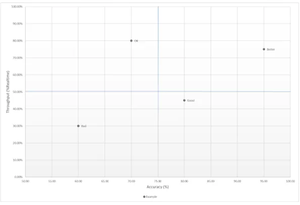
• What is the joint quantitative relationship between throughput and accuracy for each of the approaches? This can be summarized and visualized by considering each the measured throughput and accuracy of each approach as coordinates in a 2D perfor-mance space. A notional example of this is shown in Figure 1.1. In this example, four

(23)

hypothetical drift mitigation methods are shown with accuracy thresholds ranging from 60% to 95% and the associated throughputs as a percentage of maximal throughput (real-time). These represent the eponymous performance envelopes measured in this study.

Figure 1.1: Example of Performance Envelope Visualization

Relevance and Significance

In the past few years, data mining on streaming inputs has risen to prominence in the pattern recognition community (Gaber et al., 2005)(Aggarwal, 2006). Specific toolkits for applying and evaluating machine-learning methods to the stream paradigm have been put forth (Bifet & Kirkby, 2009). While, techniques to evaluate stream classifiers that react to concept drift have been proposed (Abdualrhman & Padma, 2015), the precise nature of the effect of drift mitigation on the throughput of an ensemble of streaming classifiers has yet to be systematically investigated. This study explores the performance characteristics of adaptive updating in an ensemble of supervised classifiers to provide quantitative advice

(24)

on architectural considerations for applying this approach in the streaming domain. The resulting performance envelopes allows system designers to make principled decisions on the suitability of various algorithms for real-time classification problems.

This study has implications beyond the direct domain of data stream mining. Improve-ments in real-time data processing of massive amounts of data would inform improveImprove-ments in other areas of Pattern Recognition, Artificial Intelligence and Machine Learning. These results are also relevant to the fields of Knowledge Discovery in Databases (KDD) and De-cision Support Systems (DSS). It is hoped that these findings will lead to improvements in classifiers for real-time and online learning problems.

Barriers and Issues

As discussed earlier, the problem of analyzing data-in-motion is inherently difficult due to several factors. The primary factor is the sheer volume of data being produced by information systems worldwide. This data is being captured because it is presumed that it will be useful. However, if it cannot be analyzed and acted on in a timely manner, then acquiring the massive quantity of measurements becomes a wasted effort. The advent of powerful portable devices has enabled ubiquitous computing. However, despite advances in storage technology, portable devices do not have the capacity to store and process extensive databases. In addition to technical barriers, there are social and political aspects of analyzing data-in-motion because of security and privacy concerns.

Even though online learning has been investigated in the machine learning community for some time, the problem of processing large-scale, continuous real-world data has come to the attention of a broader community in the past three to five years. Stream mining techniques have been an active topic of investigation but no standard solution to efficient stream classification, especially on non-stationary data, has been arrived as yet.

As data production and collection continue to be applied to more segments of the pop-ulation, it is critical for practical data mining techniques to keep up with a rate of data

(25)

collection that continues to out-pace the capacity to store it. The goal of this research is to investigate analytic methods that will scale along with this increase.

Assumptions, Limitations and Delimitations

These experiments operate under the assumption that the input data consists of a series of real-valued inputs collected at discrete intervals of time. For simplicity, these intervals are uniformly spaced and an input value will always be available at time t.

An essential feature of this study requires that the distribution of the underlying data changes over time. An assumption is that the sampling experiment is conducted over enough time samples for the distribution change to have a noticeable effect on the classification model. The adaptive mitigations to these concept drifts described in this report are limited to systematic shifts. The underlying distribution of the data must retain enough structure that a model can be formed. This model is subsequently invalidated when the distribution changes again. Corrections are applied to produce a new model when the system determines that the error rate of the current classification model has reached an unacceptable level.

Throughput is a primary metric examined in this study. Since the heterogeneous ensemble used by DWM, described further in Chapters 2 and 3, depends on multiple classifier types, each with different intrinsic classification rates, the throughput of the ensemble is limited by the throughput of the individual classifiers. In the simplest case, the maximum rate of the ensemble is no greater than the maximum rate of its slowest component classifier. This is controlled for by assuming the processing rate to be averaged over a sufficiently large time interval that the result accurately reflects the long term performance of the system.

Also, the rate at which inputs are presented to the classifier represents an upper-bound to the maximum throughput. This is controlled for by measuring the rate of a null-processor (i.e. the stream input instances are generated but not processed). This gives the “unburdened” baseline rate of the stream processing to which each classification strategy can be compared.

(26)

Definition of Terms

Adaptive mitigation – changes made by the system to improve performance of the clas-sifier when the error rate is determined to be too high.

Binary classification – automated categorization of input data into two categories. Each item of input is assigned to either Class 1 or Class 2.

Classifier – a function that assigns a category to an input vector. Classifiers are developed by applying a training algorithm that examines example input data and builds a model to assign categories to previously unseen data. If the examples are provided with correct labels already assigned, the training algorithm is known as supervised learning. If no labels are provided, the examples are partitioned into categories based on intrinsic features of the data. This training method is called unsupervised learning.

Concept drift – a change in the class definitions over time. For this study time is measured in discrete intervals. Thus, an input that belonged to one category at time t now belongs to a different category at timet+n, wheren ∈_Z.

Ensemble classifier – a classifier function that uses the results of several independent classification models to decide the category label of each input. Various strategies can be employed by an ensemble classifier to adjudicate the final answer. Most often it involves some form of weighted average of the outputs of the component models.

Major Trial – a complete set of experiment data comprising results from all six candidate classifiers in all six (3 drift rates×2 dimensonality) experimental conditions.

Prequential Evaluation – a streaming classifier evaluation paradigm where instances from the stream are used first to test and then to train the streaming classifier. Accu-racy is determined either in a sliding window or in some cases from the beginning of the stream output.

(27)

Streaming data – data that are produced, transmitted or recorded sequentially. The data stream is formatted as a time series where time can be interpreted as continuous (as in streaming video) or discrete as in periodic sensor measurements. A data stream can be denoted formally as a series of ordered pairs (x, t) wherexrepresents ann-dimensional data vector (x ∈ _Rn_{) and} _t _{represents its associated time-stamp (}_t _∈

Z for discrete cases; t∈_R for continuous scenarios).

Throughput – a measure of the amount data processed per unit of time. The granularity of elements processed and time units are defined in the context of the task.

Summary

In order to gain insights on efficient means for categorizing massive amounts of data, various algorithms for supervised binary classification including ensembles with drift detection were applied to a sequence of data with an underlying distribution that evolves in time. The classification models were compared in terms of accuracy and throughput. The detailed time course of shifts in accuracy was also examined. The insights gained in this study can be used to recommend improved methods for working with massive stream-based data sources.

(28)

Chapter 2 Review of the Literature

Real-time Pattern Analysis

One of the most challenging aspects of data stream mining are the time and space constraints of processing massive amounts of data in real-time. The data typically arrive at a rate that is too rapid to store and process offline. The relevance of the data may also have a short time window. An example of this situation is the analysis of real-time sensor data. Also, in some problem domains, the features of the data being analyzed may be expected to change in time. In these cases, analyzing historical data may do more harm than good (Dulhare & Premchand, 2010).

In many real time systems, data is not stored once it is processed (Bifet & Kirkby, 2009). This constraint means that machine learning evaluation techniques such as n-fold cross-validation and classical, iterative machine learning paradigms such as Self-Organizing Maps (Kohonen, 1982) which require several passes over the data examples are not applicable. New techniques must be feasible in the single-pass case. The single pass paradigm of stream mining also includes the goal of processing incoming data at or faster than the rate of arrival (Gaber et al., 2005).

Trainable pattern recognition systems are categorized as supervised orunsupervised de-pending on whether the classifier function is built by incorporating examples that are ex-plicitly labeled with the target class (Bishop, 2007). In the supervised case, the system is architected to minimize the error between its output in response to an input set and a set

(29)

of known target outputs for the same input set.

For stream processing, observations that provide discriminative features of the categories to be learned may only become available over an extended time course. Also, the categories of interest commonly evolve in time. This leads to the phenomenon of concept drift (Becker & Arias, 2007). Unsupervised methods, which do not depend on ground truth, can also be used in an attempt to discover patterns in the input values. These require the definition of a measure of similarity between inputs. The inputs are transformed into a vector space model that facilitates distance measurements. Items close to each other in this space are considered members of the same class. This is known as clustering. Applying appropriately defined distance measurements is central to the success of these methods and new metrics are being researched and refined (Aggarwal, 2003). Stream-friendly adaptations to clustering include incremental vs. hierarchical and iterative methods (e.g., k-means) commonly used on data-at-rest (Ruiz, Menasalvas, & Spiliopoulou, 2009).

The non-stationary nature of data streams also requires adaptations in unsupervised clustering techniques where the cluster centers must be continuously updated in light of new data (Gaber et al., 2005). Clustering can also be considered multi-class classification. In that sense, real-time incremental feedback may also pay a role in improving clustering.

Ensemble Classifiers

As with static data mining solutions, the approach of combining the outputs of multiple classifiers has been used to increase accuracy on data stream analytics. In an influential study (D. H. Wolpert & Macready, 1997), it was shown that no single model used for classification can provide optimal accuracy on all data that could be used as model inputs. The essential argument became known as the “no free lunch” theorem.

The solution to this issue is to devise methods of combining multiple classification models and has become a well-established method to improve correct classification of input. The optimal combination is accomplished by applying several models to the same input set and

(30)

adjudicating the responses to create systems called ensemble classifiers. Ensemble classifiers have since been shown to consistently outperform single classification models (Bauer & Kohavi, 1999) (Breiman, 2001).

The ensemble approach has been used in stream based classification problems to detect and manage concept drift in the streaming data by deferring decisions on the input data until several examples have been aggregated by the ensemble (Masud et al., 2010). The loss of discriminating features is a possible adverse consequence of aggregation and averaging.

The diversity of the classifiers in the ensemble has also been shown to be a significant factor in creating robust machine learning systems for data streams since they have been found to maintain a lower error rate after the onset of a concept drift event (Minku et al., 2010). This study uses a variety of supervised classification models that have proved success-ful in a variety of problem domains. The strengths, weaknesses, and adaptive modifications of various types of supervised classifiers is discussed below. The stream-friendly versions of these algorithms are either present in the MOA toolkit or readily implemented using MOA’s extension API.

Selected Supervised Classifiers

This section is divided into subsections that briefly review the characteristics of the classifica-tion algorithms used in this study. These algorithms are relevant to the overall architecture and listed in no particular order. Further algorithmic details specific to the experiment frame-work configuration are provided in Chapter 3. The basic operating principles, strengths, and weaknesses are briefly summarized.

Na¨ıve Bayes (NB)

Basic Principle – The Na¨ıve Bayes classifier rule estimates classes of the given input based on probability distribution of examples provided in training.

(31)

target classesCkis denoted Pr(x|Ck). These are computed from the target class labels associated with the example feature values in the training set. Then the posterior class probabilities are determined using Bayes’ theorem in the form shown in Equation 2.1 (Bishop, 2007). Pr(Ck|x) = Pr(x|Ck) Pr(Ck) P kPr(x|Ck) Pr(Ck) (2.1)

Strengths – The model is efficient and can obtain the probabilities directly from the data without extensive preprocessing. Because the model is inherently probabilistic, a quan-titative measure of confidence in the decisions is available.

Weaknesses – The term “na¨ıve” in the name refers to the assumption of conditional inde-pendence. This assumption may not hold in the actual data leading to misclassification. Adaptive Update Mechanisms – For Bayesian classifiers, online bagging and boosting (Oza & Russell, 2001) methods have been described that only require one pass through the training data as opposed to the multiple sampling from a static batch that these processes usually require. Online boosting in particular can be applied to this classifi-cation algorithm to update the current model based directly on the previous misclassi-fication. The window of relevant results was adjusted dynamically as described below and in Chapter 3.

Support vector machines

Basic Principle – Support vector machines (SVM) are a classification method that searches for a decision surface that maximally separates the exemplars from each of two classes. The examples from each class that determine the margin are known as “support vec-tors.”

(32)

de-cision model is linear of the form shown in Equation 2.2 (Bishop, 2007).

y(x) =wTφ(x) +b (2.2)

Training examples are given as a set of n input vectors {x1, . . . , xn} and associated target values {t1, . . . , tn} taken from the binary set of class labels {−1,1}. The φ(x) are fixed transformation functions (kernels) that may be applied to convert the feature vectors to a form that aids optimization of the model. The weight (w) and bias (b) parameters that maximize the margin are then derived as a quadratic optimization problem (Chang & Lin, 2011). The trained classifiers have a target output given by:

y(xn) =        <0 if tn<−1 >0 if tn≥1 (2.3)

Thus the binary classification is performed on each unknown input x by examining the value of sgn(y(x)) and assigning one class label to inputs that map to positive values and another class label to inputs that map to negative values.

Strengths – SVM training selects the model that maximally separates the classes. This should lead to lower misclassification rates. The properties of the SVM model and training procedures have been theoretically analyzed (Burges, 1998) and shown to have good generalization properties.

Weaknesses – SVM is an inherently binary classifier and multiple instances must be de-ployed serially or in parallel to perform multi-class classifications. The basic SVM model is linear and assumes that the classes are linearly separable. Non-linear class boundaries cause misclassification errors. Modifications to linear classifiers to handle such cases can be made by using non-linear basis functions.

(33)

quential versions of SVM are also available (W. Wang, Men, & Lu, 2008). The se-quential approach starts with an initial set of data points and finds an optimal kernel transformation to apply to the SVM model given the current examples. Each new data point from the stream is checked for consistency with the current model utilizing a set of vectors orthogonal to the support vectors transformed by the current kernel. If the new point falls outside the bounds of the optimal model the optimization process is repeated otherwise the model remains unchanged. In a direct comparative study, in addition to learning in real-time, the online SVM approach showed a lower error rate than batch SVM (W. Wang et al., 2008). The MOA stream version of the SVM classifier, based on an optimized gradient solver (Shalev-Shwartz, Singer, & Srebro, 2007) known as Pegasos (PEG), was used for the experiments in this study.

Hoeffding trees

Basic Principle – Hoeffding Trees (HT), invented by Domingos and Hulten (2000) are a variety of decision tree classifiers and thus share the basic operating principles of decision trees. The classical decision tree learns a set of classification rules by analyzing example feature vectors and inducing rules based on the feature values that lead to correct decisions. The HT algorithm is named after the Hoeffding bound which is utilized to decide whether or not to split on a feature. This theoretical bound, used in HT, states that for n observations with a given range of values R, the difference between the sample mean and the true mean is no greater than where:

= s

R2_{ln (}1

δ)

2n (2.4)

The condition is guaranteed with probability: (1−δ) (Domingos & Hulten, 2000). Operational Method – During training of a classical decision tree, features that separate

(34)

of decision nodes in the tree by using the most informative attributes to split on in terms of information gain. Information gain is defined by measuring the entropy of the classes discriminated by the splitting rule (Bifet & Kirkby, 2009). The entropy of a set of n partitions of the class labels is shown in Equation 2.5. The partition is given as a distribution of fractional values (pi,{1≤i≤n}) that sum to 1.

n

X

i=1

−pilog2(pi) (2.5)

Hoeffding Trees allow the decision tree to be constructed on the fly from examples examined one at a time. The inventors of the HT show that decision tree rules can be constructed using sufficient statistics instead of storing the examples themselves. For the HT algorithm the sufficient statistics are counts of the class label that co-occur with each attribute value. Thus, this classifier works most efficiently on attributes with a limited range of discrete values. The most informative feature is selected to split on among the top two candidates by choosing the one whose average information gain is greater within the bound given above.

Strengths – As with classical decision trees, an advantage of the HT is that the decision rules are explicit and provide the human user with a transparent explanation of the classification process. The conclusion justification can be vetted by the user to see if the decision process seems to be sensible or accidental. It can also expose features of the problem that may not have been readily apparent to the user. Another strength is that they operate efficiently. The average case complexity on n examples with m attributes is O(mnlog(n)) (Bifet & Kirkby, 2009).

Weaknesses – If deployed naively, the HT would try to reevaluate the splitting rules at every time step which incurs a computational cost. Additional methods are needed to decide when to incorporate new examples to adjust the rules. Exploring ways to effectively adjust the training interval is one of the prime goals of this study.

(35)

Adaptive Update Mechanisms – The incremental learning provided by Hoeffding trees has been extended as Hoeffding Adaptive Trees (HAT) to incorporate active detection of and response to concept drifts (Bifet & Gavalda, 2009). Adaptation depends on change detection which is provided by adding sentinels to each node in the Hoeffding Tree. The most straightforward sentinel is based on the ADWIN algorithm(Bifet & Gavalda, 2007). ADWIN monitors a window of recent examples and tests the hypoth-esis that sub windows do not significantly differ. If this null hypothhypoth-esis is rejected then the older portion of the window is dropped. The adaptive trees show a lower memory footprint than comparable methods however there is a definite slowdown incurred by the adaptation (Bifet & Gavalda, 2009).

Adaptive Windows for Retraining Examples

An established approach to dealing with non-stationary concept spaces has been to apply techniques from statistical time series analysis (Gaber et al., 2005). This study uses an ensemble of such adaptive classifiers designed for concept-drifting data.

Adaptive correction begins with detection of the drift away from accuracy. Once the drift is detected, it is important to determine a set of recent examples that provide a representative sample to update the classification model. A common technique is to update the classifiers based on data collected within a window of time whose length depends on the current accuracy (Bifet et al., 2010). Another approach to time uses hierarchical structuring of time periods of different resolutions. This structure provides a mechanism to facilitate the efficient detection of drifts. The adaptive approach used to determining the update window of relevant examples is described next in Chapter 3.

(36)

Prequential Accuracy Analysis

Prequential accuracy analysis is the most commonly used method to evaluate streaming classifiers (Bifet et al., 2010). Each instance in the input stream is first used to test the clas-sifier’s performance then as a new training example for the classifier. The windowed version used in this study sampled the current accuracy periodically and reported the percentage of instances correctly categorized by each algorithm over a sliding window of the past 10,000 examples classified.

Concept Drift Mitigation Strategies

The following set of concept drift correction algorithms were applied and compared at varying rates of drift to determine the relative efficiency of the approaches. Empirical findings are presented in Chapter 4 and implications and recommendations are discussed in Chapter 5.

Dynamic Weighted Majority (DWM)

This method was introduced by Kolter and Maloof (2007) in one of the first studies to specifically address concept drift in the context of ensembles of stream classifiers. The algorithm adaptively adjusts the weighted contribution of each member classifier referred to as a decision-making unit (DMU). A specification of the algorithm is given in Algorithm 2.0.1. The following is a key to the notation given in the algorithm listing.

{< ~x, L >}n – A set of n training instances (pairs of feature vectors,~x and associated class labels, L);

c∈_N – The number of classes, c≥2;

β - The factor for decreasing weights, 0≤β <1; θ - The threshold for deleting DMUs;

p - The period between DMU removal, creation, and weight update;

{< d, w >}m - A set of m DMUs and their weights; Λ, λ∈1, ..., c - global and local class predictions;

(37)

~

σ ∈_Rc _{- The sum of weighted predictions for each class.}

Algorithm 2.0.1 Dynamic Weighted Majority (Kolter & Maloof, 2007) 1: procedure _dwm({< ~x, L >}n, c, β, θ, p)

2: m ←1

3: dm ←createNewExpert()

4: wm ←1

5: for i←1, ..., n do . Loop over examples

6: ~σ←0

7: for j ←1, ..., mdo .Loop over DMUs

8: λ←classify(dj, ~xi)

9: if λ 6=yi and i modp= 0 then

10: wj ←βwj 11: end if 12: σλ ←σλ+wj 13: end for 14: Λ←argmax_jσj 15: if i mod p= 0 then 16: w←normalizeWeights(w) 17: d, w←removeExperts(d, w, θ) 18: if Λ6=yi then 19: m ←m+ 1 20: dm ←createNewExpert() 21: wm ←1 22: end if 23: end if 24: for j ←1, ..., mdo 25: dj ←train(dj, ~xi, yi) 26: end for 27: output Λ 28: end for 29: end procedure

The Accuracy Updated Ensemble Algorithm (AUE)

This method was introduced by Brzezinski and Stefanowski (2014) and aimed to be robust against various types of concept drift. A specification of the algorithm is given in Algorithm 2.0.2.

(38)

Algorithm 2.0.2 Accuracy Updated Ensemble (Brzezinski & Stefanowski, 2014)

Require: : S: data stream of examples partitioned into chunks, k: number of ensemble members, m: memory limit

Ensure: : E: ensemble of k weighted incremental classifiers 1: E ← ∅;

2: for all data chunks Bi ∈S do

3: C0 ←new component classifier built on Bi ;

4: wC0 ← 1

M SEr+;

5: for all classifiers Cj ∈E do

6: ApplyCj on Bi to derive M SEij; 7: Compute weightwij,wij = _{M SE}_r₊_{M SE}1 _ij₊; 8: end for 9: if |E|< k then 10: E ←E ∪C0; 11: else

12: Substitute least accurate classifier in E with C0; 13: end if

14: for all classifiersCj ∈E\C0 do

15: Incrementally train classifier Cj with Bi ; 16: end for

17: if memoryUsage(E)> m then

18: Prune (decrease size of) component classifiers; 19: end if

(39)

The Accuracy Weighted Ensemble Algorithm (AWE)

This method was introduced by Wang (H. Wang et al., 2003) and is designed to adapt to concept drift by re-weighting the ensemble based on the expected accuracy of its members. Expected accuracy in this algorithm can be looked at from two perspectives. The costs of the errors or the benefits of correct classifications. The costs based approach computes the mean squared error of the classifier in question (M SEi) against the mean squared error of a classifier that gives random answers (M SEr). These are computed as:

M SEi = 1 Sn X (x,c)n (1−f_ci(x))2 M SEr= X c p(c)(1−p(c))2, (2.6)

wherep(c) is the probability of an input xbeing classified as class c. The benefits approach assumes that you have assigned a numerical benefit for each classification of classcas being class c0, denoted bc,c0, and that we know the probability given by classifier C_i that input x belongs to class c, denoted as fi

c(x). The benefit is then computed as:

bi = X (x,c)n X c0 bc,c0 ·f_ci(x) _(2.7)

(40)

Algorithm 2.0.3 Accuracy Weighted Ensemble (H. Wang et al., 2003)

Require: : S: dataset ofChunkSizefrom the incoming stream,K: the number of ensemble members, ξ: number of bins, C: a set of K previously trained classifiers

Ensure: : C: a set of of K incremental classifiers with updated weights, µ,σ:mean and variance for each stage and each bin

1: train classifier C0 from S

2: compute error rate/benefits of C0 via cross-validation on S

3: derive weight w0 forC0 using wi =M SEr−M SEi, as in equation 2.6 orwi =bi−br as in equation 2.7

4: for all Ci ∈C do

5: apply Ci onS to derive M SEi orbi ; 6: Compute weight wi as above;

7: end for

8: C ←K of the top weighted classifiers inC∪C0; 9: return C

Summary

This chapter provided an overview of the methods and algorithms that have been published in the literature for designing ensemble stream classifiers. Several mitigation strategies for concept drifts were described and selected for further evaluation in this study. The next chapter discusses the design and specification of the experimental framework used to com-paratively evaluate the performance of these approaches.

(41)

Chapter 3 Methodology

Overview

This investigation was conducted in the form of an empirical study of the relationship be-tween throughput and error rates in supervised data stream classifiers including adaptive ensembles that update their classification model in an attempt to maintain accuracy when the underlying patterns in the data change. Experiments were executed using the MOA framework (Bifet et al., 2010) as well as custom scripts for experiment management writ-ten in Python. Other software utilities were used in data analysis to derive statistics and generate graphics including Matlab, Microsoft PowerPoint and Microsoft Excel.

The MOA framework provides built-in functions for the deployment and evaluation of stream based classifiers. These include adaptation of bagging and boosting methods on ensembles of Bayesian classifiers (Bauer & Kohavi, 1999) and an adaptive online version of decision trees known as Hoeffding Adaptive Trees (HAT). In this study, 3 classification model types discussed in Chapter 2 – Na¨ıve Bayes (NB), Pegasos Support Vector Machine (PEG), and Hoeffding Adaptive Tree (HAT) were used alone or in conjunction with the 3 adaptive ensemble methods to solve a binary classification problem on streams. The Adaptive Weighted Ensemble (AWE) was configured with five independent HAT members. The Adaptive Update Ensemble also comprised five HAT members. In data plots, the abbreviations AUE5 and AWE5 refer to these configurations.

(42)

method (Brown & Kuncheva, 2010) and using a heterogeneous set of classifiers made it possible to investigate independent trends in the evolving accuracy of each model type vs. the accuracy of the combined classification produced when ensembled. The Dynamic Weighted Majority (DWM) ensemble provided by MOA allows for the arbitrary specification of member classifier types. The DWM for this study was set up as a heterogeneous collection consisting of two HAT, two PEG, and one NB. In contrast, the MOA implementation of AWE and AUE only allowed ensembles of classifiers in a format compatible with Hoeffding Trees. Thus, those ensembles were assembled from five HAT classifiers.

There were four major trials executed on three separate machines. The specification of the experiment hardware is detailed below. In each major trial, The same data stream was presented to both the individual classifiers and the ensembles by using the same seed in the pseudorandom generator that creates the stream. As discussed above, the goal is to discover which algorithms produce accurate answers while preserving the maximum throughput. De-veloping and testing reliable and repeatable methodologies to evaluate and rank data stream classifiers was a major motivation for this research.

Experiment Framework

The availability of real-world test data is limited for stream analyses. The underlying nature of the data-in-motion problem requires that data be delivered to the classifier indefinitely. Thus, the data streams for this study were generated in real-time by a concept drift gen-eration simulation framework. As discussed above, the freely available MOA software was designed to support such experiments. MOA library functions, with systematically varied parameters, were used to provide the stream data to be classified. In particular, the gener-ators.RandomRBFGeneratorDrift() function of the MOA framework were used to create a stream of classification examples drawn from a mixed RBF distribution. A fixed number of centroids (using the MOA default of 50) are generated at random. Each centroid is randomly assigned to an initial class label. Examples are then generated by selecting a random

(43)

direc-tion and displacement of the example vector from the centroid. Concept drifts are induced in the model by moving the centroids away from their initial positions at a fixed drift rate specified by thedriftRate parameter listed below.

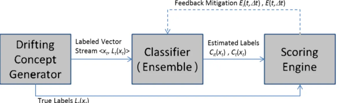
The overall conceptual architecture of the experiment framework is shown in 3.1. Each component is then explained further below. In the simulation provided by the experiment framework, time is measured in discrete steps and each value of the input, true class label, and estimated class are indexed by the current time step t. The experiment start is denoted t = 0 and N is the time step at which the experiment is shut down. Individual features in the n-dimensional data vector, at timet, are denoted: xit;{1≤i≤n}.

The ground truth label is determined by the RBF Model. The estimated label produced for inputxt by the classifier, at time t, is denotedCt(xt) and in the case of ensembles is the adjudicated decision derived from combining individual classifiers: Cit(xt);{1≤i≤5}.

Figure 3.1: Experiment Framework Architecture

Drifting Concept Generator (DCG)

• Inputs – This is the first element in the pipeline and requires no input data.

• Parameters:

– mSeed – The seed for the MOA random model generator – iSeed – The seed for the MOA random instance generator

(44)

– numAttributes - The dimensionality of the generated instances

– driftRate – The speed of centroid movement. Centroid positions are perturbed in a random direction at a rate specified by this parameter.

• Outputs – The DCG outputs a labeled stream of n-dimensional vectors. At each time step t, the DCG outputs the pair: hxt, Lt(xt)i, whereLt(xt) is the class label from the set{class1,class2} and xt is then-dimensional feature vector consisting of real-valued components xit;{1≤i≤n,0≤t≤N}.

The Drifting Concept Generator (DCG) component produces the labeled stream of data for the classification system to examine and classify. Input data were generated by using the MOA generators.RandomRBFGeneratorDrift() function to create a stream of random real-valued data vectors. The vectors at each instance are drawn from from ann-dimensional space clustered into normally distributed densities in hyperspherical regions around randomly positioned centroids. Each centroid g` has its own associated class label, `, and standard deviation initialized when the experiment begins. The data dimensionality was set to 10 and 50 for different conditions as described below. For this study, the standard deviations of each class distribution were set to the framework’s default value. The random number generator seeds were set to a fixed, user-specified value during each major trial to allow for repeatability of particular experiment runs.

The DCG simulates the existence of categories in data by assigning labels to each vector. The n-dimensional vectors xt are generated as a random displacement dt from a randomly selected centroid g`t, Lt(g`t) = `, where ` is the concept label from the set {class1,class2} that was assigned to the cluster. Thus, the stream instance at time t is given by Equation 3.1 while the label for this instance is the label of its parent cluster given by Equation 3.2.