How To Predict A Call Capacity In A Voip System

Predictive Modeling

in a VoIP System

Ana-Maria Simionovici

, Alexandru-Adrian Tantar

, Pascal Bouvry

, and Loic Didelot

b_{MIXvoip S.a, Luxembourg}

Abstract—An important problem one needs to deal with in a Voice over IP system is server overload. One way for pre-venting such problems is to rely on prediction techniques for the incoming traffic, namely as to proactively scale the avail-able resources. Anticipating the computational load induced on processors by incoming requests can be used to optimize load distribution and resource allocation. In this study, the authors look at how the user profiles, peak hours or call pat-terns are shaped for a real system and, in a second step, at constructing a model that is capable of predicting trends. Keywords—particle algorithms, prediction, user-profiles, VoIP.

1. Introduction

In the past few years, many researchers focused on de-ploying and improving the Voice over IP (VoIP) technol-ogy. VoIP platforms are subject to extremely fast con-text changes due to the dynamic pricing and automatic negotiation, availability and competition for resources in shared environments. One thus needs to provide power-ful prediction models that are able to automatically evolve and adapt in order to consistently deal with the varying nature of a VoIP system. Furthermore, as such systems generally do not allow having a centralized management, mainly due to scale concerns, one would also like to have a modular approach for, e.g., resource allocation or load balancing [1].

This study is built on a collaboration between the Univer-sity of Luxembourg and MixVoIP, a company that hosts and delivers commercial VoIP services, with an important market share in the Luxembourg area and, at this time, a significant number of subscribed clients [2]. The clients of MixVoIP are small businesses, libraries, small compa-nies. VoIP is any type of technology that can transmit, in real-time, converted voice signals into digital data pack-ets over an IP network. A VoIP service, e.g., as imple-mented and provided by a public or private company, al-lows placing calls over the Internet via an ordinary phone or computer. A VoIP phone only needs to connect to a home computer network using a special adapter. One of the main advantages of using VoIP in enterprises for example is the reduced cost of sharing a certain number of external phone lines, furthermore avoiding the allocation of a line per user. The most well known telephone system capa-ble of switching calls and of providing a powerful control

over call activity (through the use of channel event log-ging) is Asterisk [3]. It is a framework for building multi-protocol, real-time communications solutions. Asterisk is in charge of establishing and managing the connection be-tween two end devices by sending the voice portion of the call and everything that is not voice, also known as overhead. The protocols in charge of controlling mul-timedia communication sessions, respectively of deliver-ing information and transferrdeliver-ing data are Session Initia-tion Protocol (SIP), and Real Time Protocol (RTP). SIP is a signaling communications protocol, widely used for con-trolling multimedia communication sessions such as voice and video calls over Internet Protocol (IP) networks. SIP is one of the most known protocols in charge of signal-ing, establishing presence, locating users, settsignal-ing, modify-ing or tearmodify-ing down sessions between end-devices. After the connection is established, the media transportation is done via RTP. Codecs are used for converting the voice portion of a call in audio packets and the conversation is transmitted over RTP streams. The calls are stored by the VoIP providers in a Call Detail Record (CDR) database for billing.

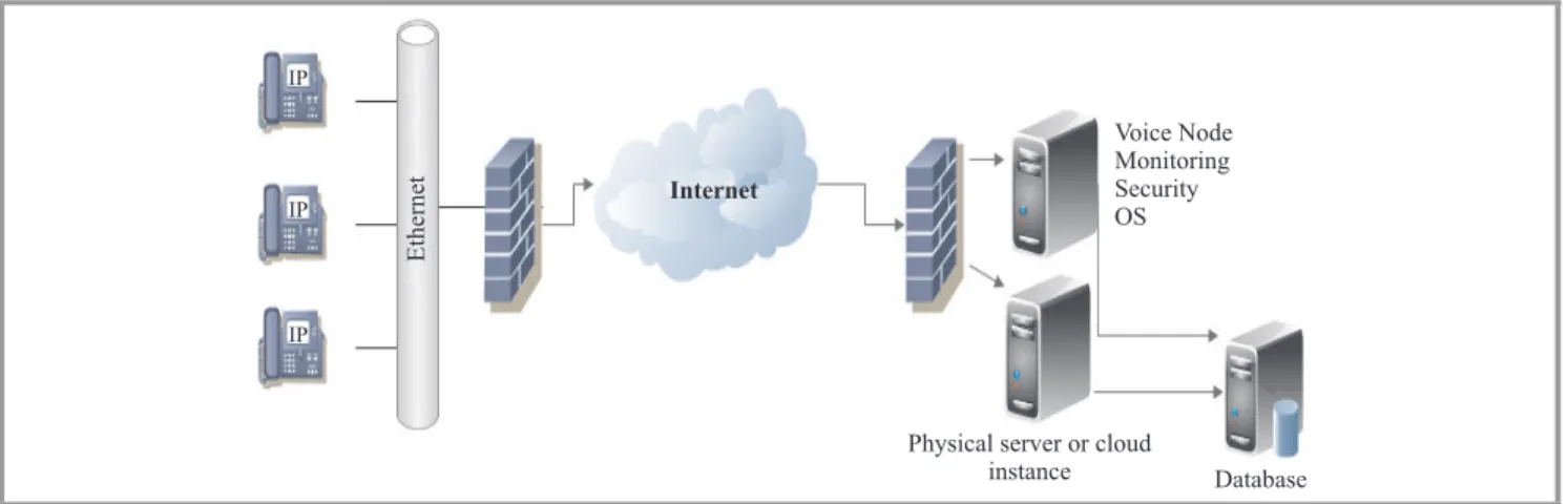
An example of a telephone system solution for VoIP is given in Fig. 1. The users connect via Internet to a server that runs either on a physical machine or in a data cen-ter or in the cloud. All users must be regiscen-tered to a SIP Registrar Server in order to indicate the current IP address and the URLs for which they would like to receive calls. The security layer can include SSH, FTP and access con-trol or sessions for password protected phone login. The voice nodes control call features such as voice mail, call transfer, conference functions. The solutions are mainly deployed on Linux distribution. After authorizing the user to place calls, two links are made. First, the user calls As-terisk that, in turn, connects to the database server in order to check the credentials of the user and if the call can be made, e.g., credit on a pre-pay account. Second, Asterisk tries to reach the other end-device. After the call is fin-ished, when the user hangs-up, call detailes are stored in the CDR (e.g. client id, destination, prefix, call duration, billing). The situation presented above stands for outbound calls placed by the users of the VoIP service provider. De-pending on the codecs of each device on the call path, the decoding and re-coding operations increases the CPU us-age. The VoIP provider is in charge of forwarding the call to different telecom operators. For incoming calls, the

car-Fig. 1. Basic example of VoIP telephone system.

rier connects to the VoIP provider which, in turn, looks up for the number and returns the number and location where the user can be reached.

Together with MixVoIP the authors work on a next gen-eration cloud-based product range, a model that adapts to and copes with the highly dynamic evolution of requests, load or other stochastic factors. At the same time, in order to deal with a model based on an extremely large number of parameters, all in a time-dependent framework we look at dynamic factors and stochastic processes while taking into account repeating activity patterns, failures, service level agreements. Thus, one needs to know how to define time dependency in order to bridge, in a coherent man-ner, online (real life) processes, the concepts employed in modeling those aspects, and the (classically) static repre-sentations used in optimization. As an example, a specific aspect one can exploit is that activity patterns inside such systems tend, over specific periods of time, to express regu-lar or localized characteristics, e.g., the evolution of energy price when relying on renewable sources, cyclic load over a 24 hours span.

The final goal of the project developed by the University of Luxembourg and MixVoIP company is to implement such an approach within MixVoIP’s environment, i.e., capable of providing a prediction system for cloud-based platform. The project can be split into two main research areas: pre-diction and load balancing. Currently, we focus on building the prediction model (in charge of anticipating the number of the calls in the system) and be used as an input for the dynamic load balancing. The transition to a direct imple-mentation for the cloud environment, to develop intelligent load balancing mechanisms that optimally spread the traf-fic inside the cloud, is therefore needed. To this end, with the support of MixVoIP, the paradigms designed inside the project will also be put into practice, hence resulting into a fully functional predictive optimization system for real cloud based VoIP platforms. The mechanism should be ro-bust, flexible and scalable. Moreover, the load balancing mechanisms should address several requirements like in-creased scalability, high performance, high availability or failure recovery.

The need for resource capabilities arises as the cost-saving benefit of dynamic scaling is brought by the cloud phe-nomenon and given that cloud computing uses virtual re-sources with a non eligible setup time. Prediction is thefore necessary. Statistical models that describe resource re-quirements in cloud computing already make the object of pay-as-you-go, e.g., providers of environments that scale transparently in order to maximize performance while min-imizing the cost of resources being used [4]. By predict-ing the load, allocatpredict-ing tasks to processors and dynami-cally turning off reserve computational resources, the high power required by cloud computing system can be reduced drastically [5].

Cloud computing can be seen as an overlay where seam-less virtualization is implemented while dealing with pri-vacy constraints. It relies on sharing computing resources rather than on having local servers or personal devices to handle applications. Cloud computing is used to increase capacity or add capabilities on the fly without investing in new infrastructure, training new personnel, or licens-ing new software. As a specific aspect, one may consider a computational demand and offer scenarios, where individ-uals or enterprizes negotiate and pay for access to resources through virtualization solutions (administered by a different entity that acts as provider) [6]. Cloud computing encom-passes any subscription-based or pay-per-use service that, in real time over the Internet, extends IT’s existing capabil-ities [7]. Demanding parties may however have diverging requirements or preferences, specified by contractual terms, e.g., stipulating data security, privacy or the service quality level [8]. Moreover, dynamic and risk-aware pricing poli-cies may apply where predictive models are used either in place or through intermediary brokers to assess the finan-cial and computational impact of decisions taken at differ-ent time momdiffer-ents. Legal enforcemdiffer-ents may also restrict access to resources or data flow, e.g., data crossing borders or transfers to different resource providers. As common examples, one can refer to Amazon Web Services [9] or Google Apps Cloud Services [10].

The impact of task scheduling and resource allocation in dynamic heterogenous grid environments, given

indepen-dent jobs has been studied in [11]. The authors developed a hierarchic genetic schedule algorithm, capable of deliv-ering high quality solutions in reasonable time; makespan and flowtime are the two objectives considered for the opti-mization problem (miniopti-mization). The algorithm improves the task execution time across the domain boundaries and the results are compared with mono-population and hybrid genetic-based schedulers. The allocation of tasks to proces-sors in new distributed computing platform is challenging when interconnecting a large number of processing ele-ments and when handling data uncertaintie. In [12] a sched-uler in charge of stabilizing this process is presented. The authors discuss an algorithm where the application graph is decomposed into convex sets of vertices and it reduces the effects of disturbances in input data at runtime. With respect to the previous considerations, the paper presents an algorithm capable of predicting the number of calls placed in a VoIP system during a given time frame. The data collected from MixVoIP is analyzed and user pro-files are outlined. It has been observed that there are pat-terns in the number of calls placed during the different hours of a day, peak hours or in abnormal situations. Dur-ing public holidays the number of calls heads to less than 10 per hour and, during a normal day, there are peak hours where the servers are overloaded or hours when the traf-fic is very low. While MixVoIP has chosen to have over capacity in order to avoid dropping the calls when there is a big traffic in the system, there are reasons to improve this approach and to implement a new model capable of adapting to the number of calls while optimally allocating resources. Statistics are used as an input for the prediction model which, based on a chosen time frame, can estimate the number of calls placed during the next time frame. The rest of the paper is organized in the following man-ner. Section 2 discusses relevant background related to prediction models, and motivates the importance of pre-dicting the load. In Section 3 the prediction model and detailed information is introduced. Section 4 presents ex-periments, results. Finally Section 5 concludes and gives remarks about future work.

2. Related Work

A series of different studies looked in the past few years on prediction models and VoIP. However, most existing approaches are based on predicting the speech quality of VoIP. The impact of packet loss and delay jitter on speech quality in VoIP has been studied for example by Lijing Ding in [13]. He proposes a formula used in Mean Opinion Score (MOS) prediction and network planning. A paramet-ric network-planning model for quality prediction in VoIP networks, while conducting a research on the quality degra-dation characteristic of VoIP, was presented by Alexander Raake in [14]. The work addresses to the different tech-nical characteristics of the VoIP networks linked with the features perceived by user. He gives a detailed descrip-tion of VoIP quality and discusses how wideband speech

transmission capability can improve telephone speech quality.

In [15] the authors present a solution for non-intrusively live-traffic monitoring and quality measuring. Their solu-tion allows adapting to new network condisolu-tions by extend-ing the E-Model proposed by the International Telecommu-nication Union-TelecommuTelecommu-nication Standardisation Sector (ITU-T) to a less time-consuming and expensive model. Another model for objective, non-intrusive, prediction of voice quality for IP networks and to illustrate their appli-cation to voice quality monitoring and playout buffer con-trol in VoIP networks is presented in [16]. They develop perceptually accurate models for nonintrusive prediction of voice quality capable of avoiding time consuming subjec-tive tests and conversational prediction voice non-intrusive models quality for different codecs.

The problem of traffic anomaly detection in IP networks has been studied in [17]. The author presents an easy closed form for prediction of the mean bit-rate of one conversa-tion generated by SID-capable speech codecs as a funcconversa-tion of the codec and the number of frames per packet used. Reference [18] explores the cumulative traffic over rela-tively long intervals to detect anomalies in voice over IP traffic, to identify abnormal behavior when different thresh-olds are exceeded.

While extensive studies exist in each of the mentioned ar-eas, only few sources consider such a holistic approach and analysis. Also, no conclusive agreement in the optimization domain exists on how to deal with highly dynamic time-dependent systems, causality and impact in a predictive framework, information coherence or descriptive power of the models when facing a fast changing environment where different scenarios are possible. Last, to the best of our knowledge, the use of such highly integrative techniques in a real world setup has not been addressed to this extent ever before and would therefore represent a premiere for the cloud based VoIP commercial domain.

3. Algorithm

The final goal of the project developed by the Univer-sity of Luxembourg and MixVoIP is to implement an ap-proach that, first, improves the VoIP service and that, sec-ond, scales to a cloud-based-solution. In this section an algorithm based on interactive particle algorithms [19] is presented, adapted, e.g., for VoIP. It allows predicting the traffic in servers, the number of calls, based on previous observations. The model is namely based on interacting particle algorithms used for parameter estimation, given a Gaussian model [20]. Pierre Del Moral and Arnaud Doucet define interactive particle methods as extension of Monte Carlo methods, allowing to sample from complex high dimensional probability distributions. The algorithm can estimate normalizing constants, while approximating the target probability distributions by a large cloud of ran-dom samples termed particles. Each particle can evolve randomly in the space and, based on its potential, can

sur-Algorithm 1Estimation of parameters pseudo-code

Generation of Particles,P(µ,Σ)

Fix some population size,N

DrawX_∼N_d(µ,Σ),

fori=1→N do

{For each particle}

Generateµ fromN _{(0,1)e.g. Box M¨uller} Determine the (lower) triangular matrix A via a Cholesky decomposition ofΓas AAT

CalculateX_←µ+AN_(0,Id),d iid variable from N _{(0,1)e.g. Box M¨uller}

CalculateΣ←∑ni=1XiX iT LikelihoodL= (2π)−N×d/2_{× |Σ|}−N/2_× exp∑Ni=1− (x−µ)T×Σ−1×(x−µ) 2 end for Perturbation of Particles fork=1→stepsdo

Perturb the encoded vectorW _{≡ {}Xi∼Nd(0,Σ)} Draw samples{Yi∼Nd(0,Σ)},1≤i≤n Construct a new vector{Xi←√a×Xi+

√

1−a_×Yi}, 1≤i_≤n

Perturbµ,µ←µ+val,valgenerated fromN_(0,1) Calculate new sigma,Σ←∑ni=1XiX iT

CalculateLnew, likelihood with newΣandµ if Lnew>Lthen

Set the new values ofΣ,µ in the particle

end if end for

Algorithm 2Prediction Step

Choose the prediction method

Select the particle with maximum likelihood and ex-tractµ andΣthat best describe the observed data Let the distribution be N_d(µ,Σ)

For Z_∼N_{d(µ,Σ)we consider the following partition:}

µ= " µα d µ_dβ # , Σd= " Σα1 d Σ α2 d Σβ1 d Σ β2 d # Zα_|Zβ =z_∼N _(µc_,Σc₎ µc_=µα d +Σ α2 d ×(Σ β2 d )−1×(z−µ β d) Σc_=Σα1 d −Σ α2 d ×(Σ β2 d )− 1_×Σβ1 d

Prediction based on the likelihood of each particle, weighted likelihood and the training test

LetLtotal=∑Ni=1L fori=1→size(samples)do Zβ= N ∑ i=1 Zα×Li Ltotal end for

vive or not. If a particle does not survive it will not be brought back. Many applications took benefit of this in-tuitive genetic mutation-selection type mechanism in areas as nonlinear filtering, Bayesian statistics, rare event sim-ulations or genetic algorithms. The sampling algorithm applies mutation transitions and includes an acceptance – rejection selection type transition phase. To this end, the approach is closely related to evolutionary-life algorithm, though while providing theoretical error bounds and perfor-mance analysis results. For a full description, please refer to the work of Pierre del Moral [19]. The algorithm starts withN particles, denoted byξi

0,1≤i≤N, that evolve

ac-cording to a transitionξi

0→ξ1i, given a fix setA. Ifξ1i∈A,

it will be added to the new population of N individuals ((ξˆi

1)1≤i≤N), else being replaced by an individual randomly fromA. The sequence of genetic type populations is defined by ξn:= (ξni)1≤i≤N selection_{−−−−−→} ξˆn := (ξˆni)1≤i≤N mutation_{−−−−−→}

ξn+1. ξˆni₋1→ξni, can be seen as a parent. An overview of convergence results including variance and mean error estimates, fluctuations and concentration properties is also given in [19].

For the estimation of parameters, a population of particles is generated as in the following. Each particle encodes a mean vectorµof sized, a matrix,W_{≡ {}Xi∼Nd(0,Σ)} sampled from a Wishart distributionW(Σ,d,n). It is used to model random covariance matrices and describes the probability density function of random nonnegative-definite

d_×d matrices [21]. The parametern refers to the degrees of freedom while Γ in Algorithm 1 and denotes a scale matrix. After generating the initial population of particles, a perturbation step is repeated for a given number of times with a pre- specified constant value, a. The perturbation step consists in modifying the parameters of each particle subject to distribution invariance constraints. We generate a new valueval fromN_{d(0,Σ)andµ←µ+val is} calcu-lated, and draw new samples {Yi∼Nd(0,Σ)}, 1≤i≤n. The encoded vector is recalculated based on vectorY and value a, as described in the algorithm. After building the new Σ, the likelihood of the perturbed particle is deter-mined. If the value of the likelihood is improved, then the perturbed particle is accepted and the old one is deleted from the population. This step is repeated for a number of times, in order to determine the values of the parameters that maximize the likelihood. The perturbation can be seen as a transition or mutation of each particle.

After the last perturbation step we get the final popula-tion. There are two prediction methods presented in Algo-rithm 2. First, the particle with the maximum likelihood is chosen, and then the parameters with the first component (Zα, input for testing) are obtained, the second component (Zβ) is extracted. Second, we take in consideration the likelihood of all the particles. The componentZβ is calcu-lated via a weighted sum of the likelihoods multiplied by the first component and divided by the sum of likelihoods. The result consists in an estimation of the traffic during the second time frame, for every working day of the chosen year.

Fig. 2. Data collection, data analysis, prediction, decision.

4. Experiments and Results

The prediction model has been trained and tested on real data from MixVoIP. In Fig. 2 is given a description of the path leading from data collection to data analysis,

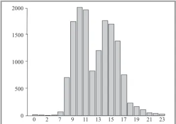
Fig. 3. The total number of calls placed in the third week of April 2012.

Fig. 4. The total number of calls placed in the second week of November 2012.

prediction and then modification of the system. The first step collects and analyzes the information from the detailed records of placed calls, e.g., the account code and profile id. One profile id can have multiple account codes. We can categorize the users based on the number of calls placed and treat the main customers with a higher priority. The destination of the call is also recorded and, after analyzing the data we are able to see that, based on the location of the specific services, the calls are more likely to be placed in that area. The duration of the calls is an useful infor-mation along with the date of the call.

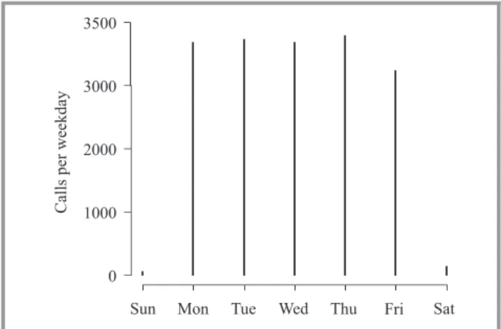
Figures 3 and 4 are two examples of the total calls placed during two different weeks from 2012. Throughout a day, the highest traffic is during working hours (8–11 and 13–18). Due the profile of the clients at MixVoIP, we can see in Figs. 5 and 6 that, over a week, the traffic is high from Monday till Friday, during working hours. Abnormal situations can be revealed if the load of the server becomes high outside the detected normal intervals and days as we can see in Fig. 7. This information is used as input to pre-dict the load of the servers during working days and peak hours. As training set, the calls placed in 2012 from hour 10 to hour 11 is chosen. We compared the accuracy of the presented prediction methods with a feed-forward neural network approach [22].

Neural networks are widely used for prediction problems, classification or control, in areas as diverse as finance, medicine, engineering, geology or physics. An artificial neural network is a computational model inspired from the structure and function of biological neural networks. It is considered to be a strong nonlinear statistical data model-ing tool where the complex relationships between inputs and outputs are modeled or patterns are found. Pattern classification, function approximation, object recognition, data decomposition are only a few examples of problems where artificial neural networks were applied. An artificial neuron receives a number of inputs corresponding to synap-tic stimulus strength in a manner that mimes a biological neuron, are fed via weighted connections, and has a thresh-old value. Each neuron can receive x1,x2, . . . ,xm inputs

Fig. 5. Distribution of calls per weekday from the first week of February 2012.

Fig. 6. Distribution of calls per weekday from the first week of August 2012.

Fig. 7. Abnormal situation, possible attack in the first week of September 2011.

that havew1,w2, . . . ,wm weights. Using the weighted sum of the inputs and the threshold, the activation of a neu-ron is composed. To produce the output of the neuneu-ron, the activation signal is passed through, the neuron acting like the biological neuron. A feed-forward [23] neural net-work is a collection of neurons that connect in a netnet-work

that can be represented by a direct graph with nodes (neu-rons) and edges (the links between them). The feed-forward neural network receives as input values that are associated with the input nodes while the output nodes are associated to output variables. Hidden layers may also appear in the structure of the network [24]. Various types of data can be predicted using neural networks, e.g., future value or trends of a variable (value increase or decrease).

In our model, each day is defined by two parameters: num-ber of calls at hour 10, respectively 11,D(X,Y). Depending on the number of segments chosen, e.g. nrSeg=300, we can calculate, for each time frame, the size of the intervals as being the maximum number of calls for hour 10, respec-tive by 11, divided by the number of segments (size1,size2)

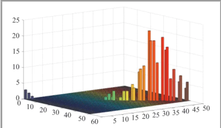
(Algorithm 3). Each day will be classified as belonging to an interval for X, respectivelyY. For, e.g., during a pub-lic holiday X andY of the respective day will equal zero. We count how many days belong to each pair (X,Y) and the classes will be used as an input for training the model (Fig. 8). After training, the calls from hour 10 have been used to test the prediction model, to anticipate the calls at hour 11.

Algorithm 3Extraction of samples pseudo-code

Store values from database in file, read file, set valuesX

andY for each day

size1=max(X)_nrSeg ,size2=max(Y_nrSeg)

Count the days belonging to each interval where(i−1)×

size1≤X≤i×size1and(j−1)×size2≤Y ≤j×size2,

i,j_≤nrSeg return samples

We generate the particles according to Algorithm 1. The number of components we use (to train the algorithm) is

d=2which defines the dimension of the space. The num-ber of degrees of freedom chosen isn=5. TheN=1000 particles will encode the vectorµand the matrixΣ. Based on the parameters of the particles and the samples used

Fig. 8. Before prediction – sample of calls placed in 2012 from 10:00-10:59 AM and 11:00-11:59 AM.

Fig. 9. After prediction – second component calculated based on the weighted likelihood of the particles.

Fig. 10. After prediction – second component calculated based on the particle with maximum likelihood.

as an input, the likelihood of each particle is calculated. This will be considered as the initial population. After the generation, for each particle the values of the param-eters µ andΣ will be perturbed according the algorithm. If the likelihood is improved, the new values will replace the old ones and move to the next step. The perturbation is applied for a number of steps, steps=100. The final population of particles will be used for prediction that is done either by considering the particle with maximum like-lihood (Fig. 9) or using the weighted likelike-lihood of the of particles (Fig. 10). For comparison, we trained and tested a neural network, using the same training set and testing set

Fig. 11. Number of predictions below a given threshold. Mean absolute percentage deviation.

(the first component) as previously discussed. The neural network has nr=10 neurons, one input, one output and two layers. We obtain the output of the neural network and we compare the prediction given by each method.

In Fig. 11, we can see a comparison of the mean absolute percentage error that was calculated using the expected out-come and the output given by the three different methods. For thethreshold_≤0.3, the neural network method has bet-ter results while for higher values, the best results are given by the average maximum likelihood. This is what interests us: the predictor that works better for higher errors. The main reasons is that, for example, minus or plus 10 calls will not make a huge difference. Miss-estimating 150 calls can have a negative impact on the system that can end up dropping calls because of lack of resources. For each method, the Mean Absolute Percentage Error (MAPE) is calculated. MAPE is used in statistics to measure the accu-racy of a method for constructing fitted time series values. MAPE is defined by the formula: M= 1

N∑ N i=1

P(i)−Z(i) P(i) , with N the size of the set, P(i) the actual value and Z(i)

the forecast value. The smaller the value of MAPE is, the better is the model. In Table 1, based on the calculated error we can see that the weighted likelihood is the best solutions and we are considering it.

Table 1

Mean Absolute Percentage Error

MAPE Value

Maximum likelihood 0.1359

Weighted likelihood 0.0998

Neural network 0.1159

5. Conclusion and Future Work

In this paper, a prediction model we have built for a real Voice over IP system is presented. The authors have namely discussed a method capable to predict the load of the traf-fic during a time frame. It was also shown that there are patterns regarding the behavior of the users when plac-ing calls. Durplac-ing public holidays, Sundays and Saturdays, the number of calls is very low while during the week-days, peaks are likely to appear. This information is helpful when taking decision regarding resource allocations. The prediction model proposed in this work combines different methodologies and will be used as an input for a future load balancing model. We also explored two different methods for predicting the load of the servers and compared the re-sults. The first one takes in consideration the entity with the maximum likelihood while the second one is a weighted likelihood based prediction. The proposed methods were compared with the prediction given by a neural network that was trained and tested with the same data.

Since the VoIP implementations and the technology in itself demand a sustained computational and bandwidth support, the decrease of operation costs at infrastructure

level is expected together with the improvement of the VoIP quality. As future work, we will compare our model with Support Vector Machines (SVM) [25], [26], an approach frequently used in machine learning community for classi-fication problems and regression analysis. SVMs are for example used for learning and recognizing patterns for a given input. Moreover, we are investigating the use of a higher number of time frames for the input and testing. We believe that adding this feature could help to improve our results. The behavior of the proposed algorithms in cases like uniformly distributed load, requests focused on one specific set of resources or fast changing profiles that switch between low and high activity periods, will also be analyzed. The idea of building a model per user is also taken into account. Depending on the period of the year, the clients are more or less active. For example, knowing that a school will be closed for summer holidays gives us the idea that less resources will be needed for that spe-cific client. Finding patterns for the normal behavior of the system and defining a confidence interval (in which the traffic can fluctuate normally) is considered. Two different situations will be distinguished: peaks in normal situations (adapt the system to scale and load balance the resources) and peaks in abnormal situations (detection and reaction against attacks). For the current experiments, the samples have been filtered and the abnormal traffic was removed from the training set.

The existing prediction model will also be extended and, based on the outcome, a highly efficient load-balancing algorithm will be developed, allowing to deal with con-straints and performance measures not addressed to such an extent and in such an integrative manner before in the literature.

Acknowledgements

This study is conducted under the support from the CNRS, France, with the National Research Fund, Luxembourg project INTER/CNRS/11/03 Green@Cloud and Luxem-bourg ministry of economy, project DynamicMixVoIP. The aims and context of this research project are built on a col-laboration between the Computer Science and Communi-cations (CSC) Research Unit, University of Luxembourg, and MixVoIP, a Luxembourg based company specialized in VoIP services.

National Research Fund, Luxembourg, http://www.fnr.lu.

References

[1] T. C. Wilcox Jr., “Dynamic load balancing of virtual machines hosted on Xen”, Master thesis, Dept. of Computer Science, Brigham Young University, USA, April 2009.

[2] Mixvoip Home page [Online]. Available: http://www.mixvoip.com/ [3] L. Madsen, R. Bryant, and J. V. Meggelen,Asterisk: The Definitive

Guide, 3rd edition. O’Reilly Media, 2011.

[4] A. Ganapathi, C. Yanpei, A. Fox, R. Katz, D. Patterson, “Statistics-driven workload modeling for the Cloud”, inProc. IEEE 26th Int. Conf. Data Engin. Worksh. ICDEW 2010, Long Beach, CA, USA, 2010, pp. 87–92.

[5] S. Kim, J.-I. Koh, Y. Kim, and C. Kim, “A science Cloud resource provisioning model using statistical analysis of job history”, inProc. 9th IEEE Int. Conf. Depend. Autonom. Sec. Comput. DASC 2011, Los Alamitos, CA, USA, 2011, pp. 792–793.

[6] M. Armbrustet al., “Above the clouds: A Berkeley view of cloud computing”, Tech. Report no. UCB/EECS-2009-28, Electrical Engi-neering and Computer Sciences University of California, Berkeley, USA, 2009.

[7] D. F. Parkhill, The challenge of the computer utility. Reading: Addison-Wesley, 1966.

[8] V. Stantchev and C. Schrpfer, “Negotiating and enforcing qos and slas in grid and cloud computing”, inAdvances in Grid and Per-vasive Computing, N. Abdennadher and D. Petcu, Eds. LNCS, vol. 5529. Berlin-Heidelberg: Springer, 2009, pp. 25–35.

[9] Amazon Elastic Compute Cloud (Amazon EC2) [Online]. Available: http://aws.amazon.com/ec2/

[10] Google Cloud Platform [Online]. Available: https://cloud.google.com/

[11] J. Kołodziej and S. U. Khan, “Multi-level hierarchical genetic-based scheduling of independent jobs in dynamic heterogeneous grid en-vironment”,Information Sciences, vol. 214, pp. 1–19, 2012. [12] A. Mahjoub, J. E. Pecero S´anchez, and D. Trystram, “Scheduling

with uncertainties on new computing platforms”,J. Comp. Opt. and Appl., vol. 48, no. 2, pp. 369–398, 2011.

[13] L. Ding, “Speech quality prediction in VoIP using the extended E-model”, inProc. IEEE Global Telecom. Conf. GLOBECOM 2003, San Francisko, USA, 2003, vol. 7, pp. 3974–3978.

[14] A. Raake, Speech Quality of VoIP: Assessment and Prediction. Chichester: Wiley, 2006.

[15] M. AL-Akhras, H. Zedan, R. John, and I. ALMomani, “Non-intru-sive speech quality prediction in VoIP networks using a neural net-work approach”,Neurocomput., vol. 72, iss. 10–12, pp. 2595–2608, 2009.

[16] L. Sun and E. C. Ifeachor, “Voice quality prediction models and their application in VoIP networks”, IEEE Trans. Multim., vol. 8, no. 4, pp. 809–820, 2006.

[17] R. Estepa, “Accurate prediction of VoIP traffic mean bit rate”,Elec. Lett., vol. 41, pp. 985–987, 2005.

[18] M. R. H. Mandjes, I. Saniee, and A. Stolyar, “Load characterization, overload prediction, and anomaly detection for voice over IP traffic”, inProc. ACM SIGMETRICS Int. Conf. Measur. Model. Comp. Sys., Cambridge, MA, USA, 2001, pp. 326–327.

[19] P. Del Moral and A. Doucet, “Particle methods: An introduction with applications”, LNCS/LNAI Tutorial book no. 6368. Springer, 2010–2011.

[20] P. Del Moral, A.-A. Tantar, and E. Tantar, “On the foundations and the applications of evolutionary computing”, inEVOLVE – A Bridge between Probability, Set Oriented Numerics and Evolutionary Com-putation, E. Tantaret al., Eds. Studies in Computational Intelligence, vol. 447. Springer, 2013, pp. 3–89.

[21] S. W. Nydick, “The Wishart and Inverse Wishart Distributions”, 2012 [Online]. Available: http://www.math.wustl.edu/∼sawyer/ hmhandouts/Wishart.pdf

[22] I. Aleksander and H. Morton,An Introduction to Neural Computing. London: Chapman and Hall, 1990.

[23] M. Budinich and E. Milotti, “Properties of feedforward neural net-works”,J. Phys. A: Mathem. Gen., vol. 25, no. 7, 1992.

[24] D. Svozil, V. Kvasnicka, and J. Pospichal, “Introduction to multi-layer feed-forward neural networks”,Chemometrics Intell. Lab. Sys., no. 39, pp. 43–62, 1997.

[25] N. Cristianini and J. Shawe-Taylor,An Introduction to Support Vector Machines. New York: Cambridge University Press, 2000.

[26] T. Joachims, “Text categorization with Support Vector Machines: Learning with many relevant features”, inProc. 10th European Conf. Machine Learn. ECML’98, Lecture Notes in Computer Science, vol. 1398. Springer, 1998, pp. 137–142.

Ana-Maria Simionovici is a Ph.D. candidate at the Uni-versity of Luxembourg. She is currently working on evolution-ary computing, prediction, load balancing. She holds Master’s degree in Computational Op-timization from University of Al. Ioan Cuza, Iasi, Romania (2012).

E-mail: ana.simionovici@uni.lu

Computer Science and Communications University of Luxembourg

Campus Kirchberg, E 009 6 rue Coudenhove-Kalergi L-1359 Luxembourg

Alexandru Tantarreceived his Ph.D. diploma in Computer Sci-ence in 2009 from the Univer-sity of Lille. He is now a Re-search Associate at the Univer-sity of Luxembourg, conduct-ing research on parallel evolu-tionary computation, the mod-eling and optimization of large scale, energy-efficient dynamic systems and Monte Carlo based algorithms.

E-mail: alexandru.tantar@uni.lu

Computer Science and Communications University of Luxembourg

Campus Kirchberg, E 009 6 rue Coudenhove-Kalergi L-1359 Luxembourg

Pascal Bouvry earned his Ph.D. degree (’94) in Computer Science with great distinction at the University of Grenoble (INPG), France. His research at the IMAG laboratory focused on mapping and scheduling task graphs onto Distributed Mem-ory Parallel Computers. He is now Professor at the Faculty of Sciences, Technology and Com-munication of the University of Luxembourg and heading the Computer Science and Communication research unit. Professor Bouvry is currently holding a full professor posi-tion at the University of Luxembourg in computer science. His current interests encompass optimization, parallel/cloud computing, ad hoc networks and bioinformatics.

E-mail: pascal.bouvry@uni.lu

Computer Science and Communications University of Luxembourg

Campus Kirchberg, E 009 6 rue Coudenhove-Kalergi L-1359 Luxembourg

Loic Didelot is the current Founder at Pindo S.a., CEO at Corpoinvest holding, Co-Owner at Forschung-Direkt Company. Since February 2008 he is also the Founder and Co-owner of MIXvoip S.A. He has compe-tences in building highly scal-able and secure products based on linux and open source solutions while considering the commercial alternatives. He has great know-how in web development (PHP, CSS, Javascript, AJAX), Linux and se-curity, Asterisk. He is interested in database applications that need to scale out.

E-mail: ldidelot@mixvoip.com MIXvoip S.a Luxembourg Z.I. Rolach