Adaptive Differential Evolution and its Application to Machine Vision

(1)

ADAPTIVE DIFFERENTIAL EVOLUTION AND ITS APPLICATION TO MACHINE VISION

A Dissertation

Submitted to the Graduate Faculty of the

North Dakota State University of Agriculture and Applied Science

By Deepak Dawar

In Partial Fulfillment of the Requirements for the Degree of

DOCTOR OF PHILOSOPHY

Major Department: Computer Science

July 2016

(2)

NORTH DAKOTA STATE UNIVERSITY

Graduate School

Title

ADAPTIVE DIFFERENTIAL EVOLUTION AND ITS APPLICATION TO MACHINE VISION

By

Deepak Dawar

The supervisory committee certifies that this dissertation complies with North Dakota State University’s regulations and meets the accepted standards for the degree of

DOCTOR OF PHILOSOPHY SUPERVISORY COMMITTEE: Dr. Simone A. Ludwig Chair Dr. Dean Knudson Dr. Anne Denton Dr. Cheryl J. Wachenheim Approved: July 7, 2016 Date Brian Slator Department Chair

(3)

ABSTRACT

Over recent years, Evolutionary Algorithms (EA) have emerged as a practical approach for solving hard optimization problems ubiquitously presented in real life. The inherent advantage of EA over other types of numerical optimization methods lies in the fact that they require much less or no prior knowledge of the objective function. Differential Evolution (DE) has emerged as a highly competitive and powerful real parameter optimizer in the diverse community of evolutionary algorithms.

The study of this dissertation is focused on two main approaches. The first approach focuses on studying and improving DE by creating its variants that aim at altering/adapting its control parameters and mutation strategies during the course of the search. The performance of DE depends largely upon the mutation strategy used, its control parameters namely the scale factorF, the crossover rate Cr, and the population sizeN P, and is quite sensitive to their appropriate settings. A simple and effective technique that altersF in stages, first through random perturbations and then through the application of an annealing schedule, is proposed. After that, the impact and efficacy of adapting mutation strategies with or without adapting the control parameters is investigated.

The second approach is concerned with the application side of DE which is used as an optimizer either as the primary algorithm or as a surrogate to improve the performance of the overall system. The focus area is video based vehicle classification. A DE based vehicle classification system is proposed. The system in its essence, aims to classify a vehicle, based on the number of circles (axles) in an image using Hough Transform which is a popular parameter based feature detection method. Differential Evolution (DE) is coupled with Hough Transform to improve the overall accuracy of the classification system. DE is further employed as an optimizer in an extension of the previous vehicle detector and classifier. This system has a novel appearance based model utilizing pixel color information and is capable of classifying multi-lane moving vehicles into seven different classes. Five different variants of DE on varied videos are tested, and a performance profile of all the variants is provided.

(4)

ACKNOWLEDGEMENTS

I would like to convey my earnestness to my primary advisor and mentor, Dr. Simone A. Ludwig for her enthusiastic and encouraging support during the pursuit of my research. This work is as much as a product of her guidance as of my own research. Not only did she guide me through the dissertation process, but also taught me the overall process of performing quality research. I cannot thank her enough for the supervision, encouragement and inspiration in developing the theory, conducting the experiment, publishing papers, and writing this dissertation. She has shown me the joys of research, and importance of life, and for this I am indebted to her.

I would like to also thank Dr. Dean Knudson and Dr. Anne Denton for serving on my graduate committee. I enjoyed discussing many aspects of this research with them and look forward to future discus-sions. They dedicated their valuable time on supporting my graduate study, and helping on my professional developments.

I would also like to thank Dr. Cheryl Wachenheim. With all of the other commitments to the university, she dedicated time to take part in my dissertation research, and provided valuable insights into the completion of my dissertation. She is one of the most helpful human beings I have ever known. It has been a privilege knowing her.

Finally, I would like to thank my family and friends for their support, understanding, and encourage-ment. I certainly wasn’t the easiest person to be around during the last year while I worked on this research, and my dissertation.

(5)

DEDICATION

(6)

LIST OF TABLES

Table Page

2.1. Performance of DEDASF, DETVSF, DEWD, and DE at 10D, 30D, and 50D, respectively. Re-ported values are the averages of 51 independent runs for each function. Error values reaching

within10−8of the global optimum of the function are reported as 0.00+E00. . . 17

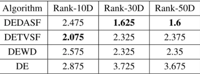
2.2. Relative Ranks obtained by DEDASF, DETVSF, DEWD, and DE at 10D, 30D, and 50D. . . 18

2.3. Friedman statistic (distributed according to chi-square with 3 degrees of freedom) andpvalue computed by Friedman Test at 10D, 30D, and 50D. . . 18

2.4. Division of benchmark functions based on their response to cooling rates. . . 20

2.5. Adjustedp-values-30D. . . 20

2.6. Adjustedp-values-50D. . . 21

2.7. Performance of DEDASF when compared to SaDE. . . 22

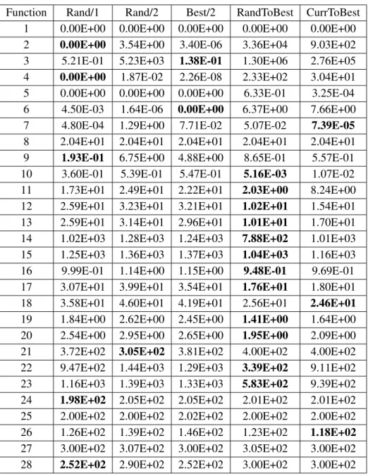
3.1. Performance of Rand/1, Rand/2, Best/2, RandToBest, and CurrToBest at 10. Reported values are the averages of 51 independent runs for each function. Error values reaching within10−8of the global optimum of the function are reported as 0.00+E00. . . 31

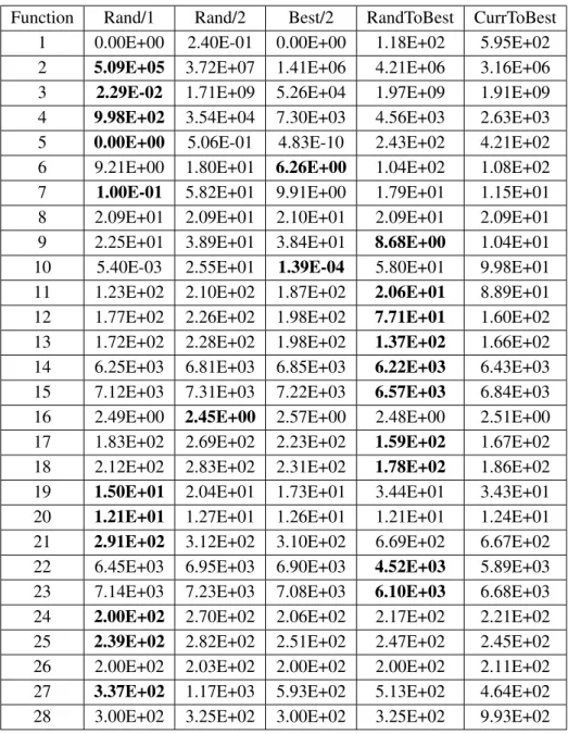
3.2. Performance of Rand/1, Rand/2, Best/2, RandToBest, and CurrToBest at 30D. Reported values are the averages of 51 independent runs for each function. Error values reaching within10−8of the global optimum of the function are reported as 0.00+E00. . . 32

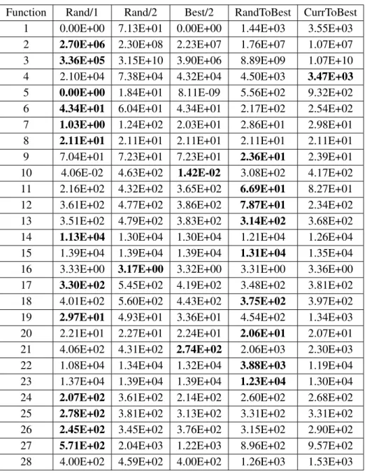
3.3. Performance of Rand/1, Rand/2, Best/2, RandToBest, and CurrToBest at 50D. Reported values are the averages of 51 independent runs for each function. Error values reaching within10−8of the global optimum of the function are reported as 0.00+E00. . . 33

3.4. Relative ranks obtained by Rand/1, Rand/2, Best/2, RandToBest, and CurrToBest at 10D, 30D, and 50D respectively. . . 34

3.5. pvalues obtained using Hochberg procedure by mutation strategies Rand/2, Best/2, RandToBest and CurrToBest when compared to Rand/1 at 10D, 30D, and 50D respectively atαlevel 0.05. . 34

3.6. Results obtained by the Wilcoxon test for strategy Rand2Best against CurrToBest . . . 35

3.7. Number of wins scored, out of 28, by all mutation strategies at 10, 30, and 50 dimensions, respectively. . . 35

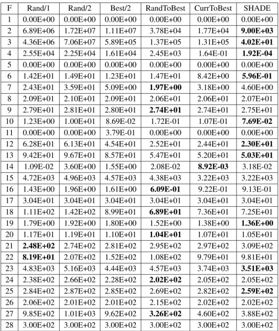
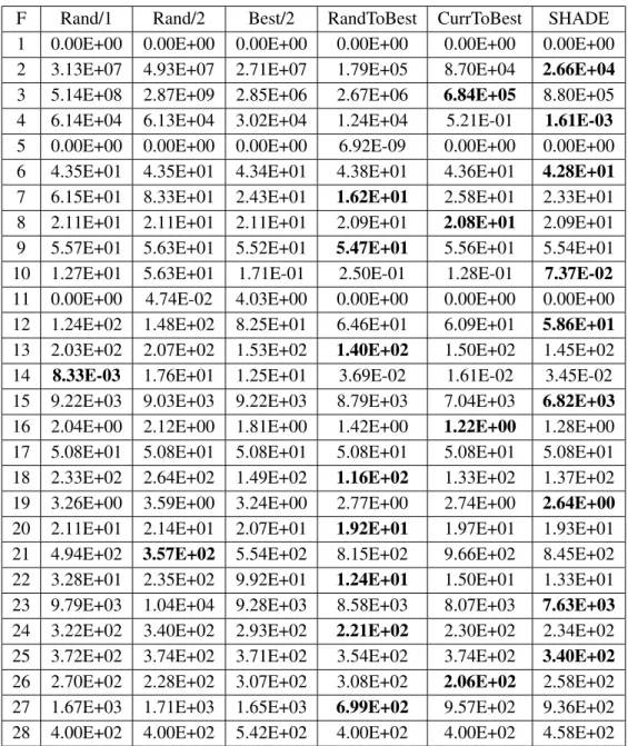
3.8. Performance of Rand/1, Rand/2, Best/2, RandToBest, CurrentToBest, and SHADE at 10D when employed with adaptive control parameter model used in SHADE. Reported values are the aver-ages of 51 independent runs for each function. Error values reaching within10−8_{of the global} optimum of the function are reported as 0.00+E00. . . 37

(10)

3.9. Performance of Rand/1, Rand/2, Best/2, RandToBest, and CurrentToBest at 30D when em-ployed with adaptive control parameter model used in SHADE. Reported values are the aver-ages of 51 independent runs for each function. Error values reaching within10−8of the global optimum of the function are reported as 0.00+E00. . . 38 3.10. Performance of Rand/1, Rand/2, Best/2, RandToBest, and CurrentToBest at 50D when

em-ployed with adaptive control parameter model used in SHADE. Reported values are the aver-ages of 51 independent runs for each function. Error values reaching within10−8_{of the global}

optimum of the function are reported as 0.00+E00. . . 39 3.11. Relative ranks obtained by Rand/1, Rand/2, Best/2, RandToBest, CurrToBest, and SHADE at

10D, 30D, and 50D. . . 40 3.12.p values obtained using Hochberg procedure by Rand1/1, Rand/2, Best/2, RandToBest, and

CurrToBest when compared with SHADE at 10D, 30D, and 50D atαlevel 0.05. . . 40 3.13. Number of wins scored, out of 28, by all mutation strategies and SHADE at 10, 30, and 50

dimensions, respectively. . . 40 3.14. Performance of parameter adaptive Rand/1, Rand/2, Best/2, RandToBest, and CurrentToBest

against SHADE, and SA-SHADE at 30D. Reported values are the averages of 51 independent runs for each function. Error values reaching within10−8_{of the global optimum of the function}

are reported as 0.00+E00. . . 45 3.15. Relative ranks obtained by Rand/1, Rand/2, Best/2, RandToBest, CurrToBest, SHADE, and

SA-SHADE at 30D. . . 46 3.16. Relative performance of SA-SHADE against state-of-the-art adaptive variants of DE at 30D.

Reported values are the averages of 51 independent runs for each function. Error values reaching within10−8of the global optimum of the function are reported as 0.00+E00. . . 47 3.17. Relative ranks andpvalues obtained by SHADE against CoDE, EPSDE, JADE, and dynNP-jDE

at 30D. . . 48 3.18. Relative ranks and p values obtained by SA-SHADE against SHADE, JADE, dynNP-jDE,

CoDE, and EPSDE at 30D. . . 48 4.1. A comparison of five variants of DE in detecting the number axles and their centers in 18 frames

isolated from multiple video sequences. The values presented indicate the best/minimum value obtained by the variant along with a binary number (successful detection is represented as 1 and 0 otherwise). . . 58 4.2. Wins, Loses, and Success Rate of multiple NP-FEs combinations for DE/Rand/1/bin tested on

18 vehicular frames isolated from multiple video sequences. . . 59 4.3. Effect of increasing NP and function evaluations on success rate. Saturation point is reported at

(11)

5.1. A comparison of five variants of DE in detecting the number axles and their centers in 20 frames isolated from multiple video sequences. The values presented indicate the best/minimum value obtained by the variant along with a binary number (successful detection is represented as 1 and 0 otherwise). . . 80 5.2. Effect of increasing NP and function evaluations on success rate. Saturation point is reported at

40-60 combination. . . 81 5.3. Confusion matrix for cumulative vehicle count across three video sequences. PV stands for

passenger vehicle. . . 81 5.4. Confusion matrix for individual classes. . . 82

(12)

LIST OF FIGURES

Figure Page

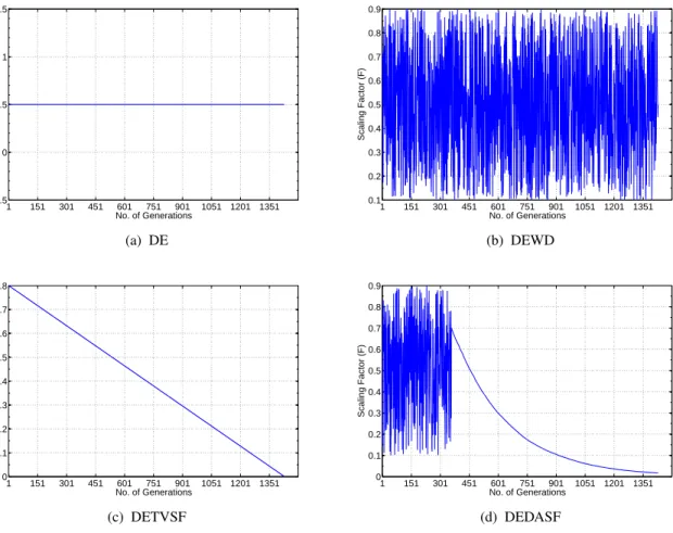
2.1. Variation in scale factor with number of generations executed for DE, DEWD, DETVSF, and

DEDASF. . . 14

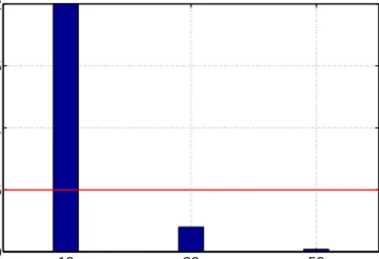
2.2. Adjusted p values obtained by Hochberg procedure for DEDASF at problem dimentionality 10, 30, and 50. DEDASF is significant at the 0.1 level of significance at problem dimensionality 30 and 50. . . 19

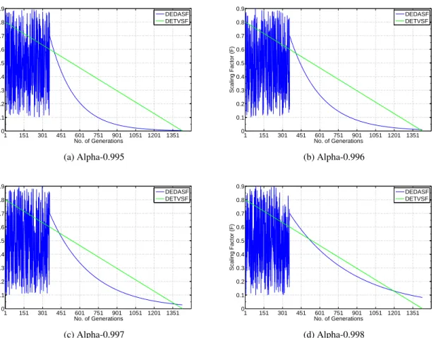
2.3. Comparison of slope of DEDASF and DETVSF at different cooling rates. . . 19

2.4. Exact p values obtained by Wilcoxon test for DEDASF when compared to DETVSF, at prob-lem dimensionality 10, 30, and 50. DEDASF is significant at the 0.05 level of significance at problem dimensionality 30 and 50. . . 21

4.1. Modular overview of the axle count based vehicle classification system. . . 53

4.2. Vehicle outlines and their associated classes. . . 57

4.3. Performance of DE/Rand1/bin using multiple population sizes with increasing function evalua-tions. . . 60

4.4. Results obtained through manual settings (left aligned) of Hough Transform parameters vs the best settings obtained for DE/Rand/1/bin (right aligned). . . 63

5.1. A typical vehicle detection system . . . 67

5.2. A typical vehicle detection system . . . 70

5.3. Change of gradient threshold during adaptive threshold calculation and updation . . . 73

5.4. A step by step description of adaptive background construction . . . 84

5.5. Vehicle detection process . . . 85

5.6. Axle detection using DE . . . 85

5.7. Vehicle outlines and their associated classes. Axle count information is necessary to distinguish between Truck Type I and II, Truck Type III and IV, and Truck Type V and VI . . . 86

5.8. Results obtained through manual settings (third column) of Hough Transform parameters vs the best settings obtained for DE/Rand/1/bin (fourth column) . . . 87

(13)

1. INTRODUCTION

Challenging real world optimization problems are ubiquitous in scientific and engineering domains. Complexity of the problem notwithstanding, the problem’s objective function may also be non-continuous, and non-differentiable adding to the overall difficulty and negotiability of the search space. Darwinian in-spired evolutionary theories like social group behavior and foraging strategies, to name a few, have attracted the attention of researchers for tackling hard and complex optimization problems. The outcome of this re-search effort are nature inspired algorithms. These algorithms can be broadly classified into two categories: evolutionary computing methods, and swarm intelligence algorithms, both of which employ their own set of control parameters.

The underlying idea behind evolutionary algorithms is the iterative fitness improvement of a popu-lation of individuals (solutions), through natural selection. An iteration generally involves, producing new individuals through a series of mutations and recombinations, gradually removing lesser fit individuals from the population and replacing them with newly generated individuals if their fitness proves to be better than the individuals they were generated to replace [1].

The operation of swarm intelligence algorithms may be behaviorally characterized as a decentral-ized swarm searching for optimal food sources (solutions) [2]. The direction of individual search is influ-enced by the current location of the individual, its best location ever, and the location of the best individual in the whole swarm.

The performance of both these classes of algorithms is quite sensitive to their respective control parameters settings, good values of which are problem dependent. Unless the user has quite an experience in parameter tuning, finding out the best parameter settings for a given problem through trial and error may prove, at best, an arduous, and sometimes an infeasible task. A way out of this conundrum lies in an arrangement that may alter or adapt these parameters during the course of the algorithm. Much attention has been paid to this problem and many adaptive schemes have been proposed [3]-[8].

One of the main motivations of this work is to intensively investigate one of the popular evolutionary algorithms namely Differential Evolution (DE), and propose mechanisms to alter-adapt its control

(14)

param-eters to improve its performance. This motivation stems from the fact that performance of DE is highly dependent on its control parameters and setting up these parameters for a given problem is a non-trivial task. The other part of this work focuses on the application side of DE. Lately evolutionary algorithms have found applications in the image processing and object tracking domains. One of the sub-domains of these problems is automatic vehicle classification. Vehicle classification is a difficult problem to tackle. Categorizing vehicles comprehensively using a video is quite an arduous task given the variety of vehicles and similarities between them at the same time. Different shapes and sizes within a single vehicle category adds to the dilemma. On top of this we have drastically changing weather conditions, shadows, camera noise, occlusions, etc., which make the task even more challenging. DE is employed as a parameter optimizer for vehicle classification and real time object tracking tasks.

The following sections briefly describe the research conducted for this dissertation. Brief descrip-tions of the background are presented in Secdescrip-tions 1.1-1.4. The motivation of the work is discussed in Section 1.5. The contributions of the work is listed in Section 1.6, and the structure of the dissertation is described in Section 1.7.

1.1. Differential Evolution

Differential Evolution (DE) [9], proposed by Storn and Price in 1995, has emerged as a robust real parameter optimizer in the field of evolutionary computation. The power and popularity of DE can be gauged from the heightened research activity on the subject in the past decade. Numerous studies have been conducted to ascertain DE’s efficacy on a broad range of problems ranging from benchmark to real life scientific and engineering problems [10]. An year after its introduction, the power of DE was on display at the First International Contest on Evolutionary Optimization in May 1996 [11], where it secured first place among evolutionary algorithms. Since then, DE and its variants have performed exceedingly well in the optimization contests such as The IEEE Congress on Evolutionary Computation and alike.

DE is simple and employs few control parameters namely scale factor (F), crossover rate (Cr), and population size (N P). The performance of DE is very sensitive to the proper settings of these parameters [1], [12], [13].

An unfavorable combination of these parameters can seriously degrade the algorithm’s efficacy. At the same time, choosing effective control parameter settings can be quite cumbersome. A good combination

(15)

of these parameters depends upon the problem at hand and requires a good amount of experience of the user. The bottom-line is, “better and more informed values of control parameters yield better results for a given problem.”

1.2. Adaptive Differential Evolution

Since it may be difficult and time consuming to generalize a set of control parameter values, there is always a motivation to alter or adapt them during the course of the algorithm as defined by certain rules. Intensive research activity has been reported in the area of finding good values of control parameters. In [1], the authors grouped this change into three broad classes:

• Deterministic -the parameters are altered based on some user defined rules [9], [14].

• Adaptive -the parameters are allowed to adapt based on some feedback from the algorithm [15].

• Self-Adaptive -the parameters are encoded into the solution itself and they evolve as a part of the general population [16], [17].

During the search process a particular combination of control parameters and mutation strategy may prove more favorable than the others [18]. As a result, many partially [19]-[21] adaptive schemes that adapt one or more control parameters, and fully adaptive schemes [22] that adapt mutation strategy and control parameters, have been proposed in the past.

The efficacy of employing an adaptive mutation strategy module both in the presence and the ab-sence of a control parameter adaptation scheme is investigated. Based on empirical results we create a pool of mutation strategies. A memory based fully adaptive version of Differential Evolution, SA-SHADE, is then proposed that adapts the control parameters to their appropriate values and chooses the best suited mutation strategy from the pool.

1.3. Video Based Vehicle Classification

Automatic vehicle classification has emerged as a significantly important element in the myriad web of traffic data collection and statistics. Regulations on road side construction for pertinent reasons, in-creasing vehicle density, and cost of overlaying roads are some of the factors calling for ever more efficient utilization of our existing transportation networks. A part of the solution to these pressures lies in vehicle classification systems that compute the number and type of vehicles passing a particular street or highway.

(16)

This information has an evident impact on the cost and efficiency of the transportation system; road thick-ness decision being one of the many advantages this system has to offer. Many video based classification systems have been proposed in the past with their own advantages and disadvantages. These systems can be primarily distinguished by the type of sensors they use, most common of which are magnetic, laser, pressure, single or multiple cameras, etc. Magnetic and laser sensors tend to have a higher classification accuracy but at the same time have high equipment and installation costs, and are intrusive techniques. Computer vision based vehicle classification systems are generally attributed with low cost and accuracy, and are an active area of research. A video based vehicle classification system is proposed that determines the type of vehicle based on the number of axles and distance between them. Hough Transform [23], a parameter based feature detection method, is employed to detect the axles. The quality of the detected circles is sensitive to appro-priate settings of these parameters. Since the process is time consuming and it may not be fruitful to adjust these parameters manually every time, there is always a motivation to do a parameter search by attaching a machine learning algorithm to discover an optimized set. This parameter search is done using DE.

1.4. A Differential Evolution Based Multiclass Vehicle Classifier for Urban Environments

This chapter rebuilds and further enhances the capabilities of video based vehicle classifier pro-posed previously. Commercial vehicle classifiers bank upon sophisticated appearance models and employ a multitude of tracking techniques for vehicle detection and classification [139]. The main idea behind vehicle detection and tracking is to estimate the motion state of an object as accurately as possible given an image sequence. A large body of research has been conducted on this topic as it finds important applications in multitude of real life areas like video surveillance, human computer interaction, and traffic flow monitoring, to name a few. Examples include a visual traffic flow monitoring system proposed in [25], pedestrian count-ing system in [26], accident detection system in [27] etc. As a part of this dissertation, a DE based multi lane vehicle detector and tracker with a novel appearance based model system is proposed.

1.5. Motivation and Problem Statement

Generally, an optimization process/algorithm, given a set of constraints, tries to find the best solution among all feasible solutions for a given problem. In real life though, there remain a large number of problems in class NP [28] for which finding the best solution is not possible in polynomial time, at least as of now. In such cases, it is more plausible to find a good enough solution (sub-optimal) instead of spending a great

(17)

deal of computational time to find the best solution. Moreover, optimization is not always about finding the perfect solution. Sometimes, it is more about finding a good solution given a set of constraints or environment. As the constraints change the solution also needs to change accordingly. This has many parallels in the Evolutionary Process.

Evolution in a way is also an optimization process wherein the solution or adaptive behavior depends upon the constraints posed by the environment of an organism. The behavior of an organism is optimized and changes according to the environment. Since evolution has been able to produce organisms of high perfection over a long period of time, there is always a big motivation behind application of evolutionary principles in the optimization process to solve hard real world engineering problems. It was due to this primary motivation that Evolutionary Algorithms (EA) came on the horizon of optimization.

Differential Evolution (DE) is a simple yet powerful evolutionary algorithm (EA) for global opti-mization introduced by Price and Storn [9]. The main motivations of this research can be summarized as follows.

• The DE algorithm has gradually become more popular among other EA’s, and has been used in many practical cases, mainly because it has demonstrated good convergence properties, and is easy to un-derstand [12]. Its success notwithstanding, DE has its own drawbacks. Its very high performance sensitivity to its control parameter settings sometimes turns out to be more of a hindrance than an asset. Improper settings of these parameters seriously degrades the DE’s performance and renders it ineffective on the problem being solved. Moreover, determining good control parameter values for every problem would either require repetitive trial & error or a good amount of user experience. These approaches in most cases are either time consuming or infeasible. Allowing the control parameters to alter/adapt themselves during the search process is, therefore, an important task. For this purpose, an adaptive control parameter mechanism for control parameters are developed.

• DE’s ability to find a good solution, apart from its control parameters, is also dependent on the muta-tion strategy it employs. A mutamuta-tion strategy determines how the chosen vectors will be differentially mutated to create a donor. Even in the presence of favorable control parameter settings, an unfavor-able mutation strategy can seriously degrade the quality of the final solution. Allowing the mutation strategy to adapt with the control parameters may help in alleviating this problem. For this purpose,

(18)

adaptive mechanisms for mutation strategies are developed that are useful both in presence, and ab-sence of adaptive control parameter mechanisms.

• On the application side, DE has been utilized in many real world domains for optimization. Video based classification of vehicles is an important task in intelligent transportation systems. Categoriz-ing vehicles comprehensively is quite an arduous task given the variety of vehicles and similarities between them at the same time. Different shapes and sizes within a single vehicle category adds to the dilemma. On top of this, drastically changing weather conditions, shadows, camera noise, occlu-sions, etc., make the task even more challenging. A DE based vehicle classifier is proposed wherein DE is used as an optimizer to improve the overall classification accuracy. DE acts as a accuracy improvement sub system. The primary axle detection mechanism is the Hough Transform which af-ter detection feeds the DE sub system. DE further validates the input and attempts to improve the accuracy of the classification system.

• Due to variety and complexity of scenes, and external noise, vehicle detection on multilane traffic is a challenging task. The performance of such a system is largely dependent upon the appearance model and tracker it uses. A number of approaches have been proposed both for appearance models and trackers. A bio-inspired multilane vehicle detection and classification system is proposed that uses a novel pixel-to-pixel color cue comparison approach for appearance modeling and DE as a discrete optimizer.

1.6. Contributions

This dissertation makes several contributions towards improving the convergence properties of dif-ferential evolution and reducing its dependency on trial & error methods to select a good set of control parameters.

On the application sides, a novel DE based vehicle classification system is proposed and later DE is is applied as real time object tracker with gaussian mixture object models. The contributions are:

1. Differential Evolution with Dither and Annealed Scale Factor (DEDASF) was devised and applied to twenty difficult benchmark functions. During the search process, the scale factor,F, was initially randomized to sample diverse areas of the search landscape, and then allowed to be non-linearly

(19)

an-nealed. This allows for random step sizes during initial exploratory stages of the search, and a gradual step size reduction during the exploitative stages. The performance of DEDASF was compared with state of the art algorithms proposed in the past. DEDASF proved to be highly competitive amongst the algorithms compared.

2. A fully adaptive version of DE, Strategy Adaptive Success History Based Differential Evolution (SA-SHADE) was proposed that is capable of adapting control parameters as well as the mutation strategy. A pool of mutation strategies was created based on empirical evidence, and successful mutation strate-gies were added to the success history. The mutation strategy to be applied in a given situation was chosen from this success history. This significantly improved the performance of DE, and reduced human intervention in setting up these parameters. SA-SHADE was compared with several state of the art adaptive variants, and was shown to be superior to most and competitive to the remainder. 3. A novel DE based vehicle classification system is proposed that utilizes the axle count, their

corre-sponding distance from each other and other parameters of a vehicle to classify the type of vehicles. Hough transform is used as a primary axle or circle detector, and DE is then subsequently used to improve the classification accuracy. Hough transform is a parameter based method that requires the parameters to be set before its operation. This requires human intervention. To alleviate this draw-back, DE is used as an automatic parameter search method. The classification system is shown to perform vastly superior in presence of DE as an optimizer when compared with the system that does not employ DE and sets the parameters manually.

4. A DE based multilane vehicle detection, tracking and classification system is proposed wherein color cues are utilized to model the appearance of the object. Multiple variants of DE are compared to ascertain robust behavior. Extensive experimental results show that DE based object tracker is robust and shows satisfactory performance for multilane vehicle detection in presence of noise, occlusion, and target deformation.

1.7. Dissertation Overview

This dissertation is a paper-based version, where each chapter has been derived from the papers published during the Ph.D. work. This is an overview of the remaining chapters of this dissertation.

(20)

In Chapter 2, a adaptive version of DE, named Differential Evolution with Dither and Annealed Scale Factor or DEDASF, is discussed. This chapter is derived from the publication:

• Deepak Dawar and Simone A. Ludwig, “Differential Evolution with Dither and Annealed Scale Fac-tor.”IEEE Symposium on computational intelligence: 9-12 Dec. 2014.

In Chapter 3, a fully adaptive version of DE namely SA-SHADE is presented. This chapter is derived from the submitted work:

• Deepak Dawar and Simone A. Ludwig, “Effect of Strategy Adaptation on Differential Evolution in Presence and Absence of Parameter Adaptation: An Investigation.”Applied Soft Computing, Submit-ted.

In Chapter 4, a novel DE based vehicle classification system is discussed. This chapter is derived from the publication:

• Deepak Dawar and Simone A. Ludwig, “A Differential Evolution Based Axle Detector for Robust Vehicle Classification.” IEEE Congress on Evolutionary Computation, May 25-28, 2015, Sendai, Japan.

In Chapter 5, a DE based multilane vehicle detection, tracking and classification system is discussed. This chapter is derived from the submitted work:

• Deepak Dawar and Simone A. Ludwig, “A Differential Evolution Based Multiclass Vehicle Classifier for Urban Environments.”International Journal of Swarm Intelligence Research, Submitted.

(21)

2. DIFFERENTIAL EVOLUTION WITH DITHER AND ANNEALED

SCALE FACTOR

Differential Evolution (DE) is a highly competitive and powerful real parameter optimizer in the diverse community of evolutionary algorithms. The performance of DE depends largely upon its control parameters and is quite sensitive to their appropriate settings. One of those parameters commonly known as scale factor orF, controls the step size of the vector differentials during the search. During the exploration stage of the search, large step sizes may prove more conducive while during the exploitation stage, smaller step sizes might become favorable. This work proposes a simple and effective technique that altersF in stages, first through random perturbations and then through the application of an annealing schedule. The performance of the new variant on 20 benchmark functions of varying complexity is reported, and compared with the classic DE algorithm (DE/Rand/1/bin), two other scale factor altering variants, and state of the art, SaDE.

The rest of this chapter is structured as follows. Section 2.1 presents an introduction to the chapter. In Section 2.2, related work is presented. Section 2.3 describes and explains the new algorithm with all its features. In Section 2.4, results and their analysis are presented, and finally, conclusions and future work are discussed in Section 2.5.

2.1. Introduction

Dither is a deterministic parameter control technique whereinFis allowed to take on random values between a specific range represented byFlowandFhigh. Combining dither with an annealing based cooling schedule to alterFis proposed, and a two stage technique, DEDASF, is introduced based on this concept. In the first stage, dither is applied and in the second stage,F is allowed to be reduced by a randomized factor. Every stage runs for a fixed number of function evaluations, a count of which has to be set beforehand. The idea is to scatter the population to diverse and favorable areas first and then reduce the step size to take advantage of the notion that during early stages of exploration of the search space by DE, large step sizes may prove beneficial for investigating the maximum area of the problem landscape, and when the exploitation stage kicks in, small step sizes may become more advantageous. Though it is possible to alternate between

(22)

exploration-exploitation during the course of the search, which may be beneficial for many landscapes, this investigation is limited to a single stage exploration-exploitation model.

2.2. Related Work

There have been many attempts to improve the performance of DE by varying the scale factor during the search process and multiple methods have been suggested to achieve this goal. One of them is Dither [14]. It is a deterministic scheme of randomization of scale factor,F. Many different ways of randomizing F are possible. For example in [29],F was randomized on a generational basis as:

Fdither =Fl+randG(0,1)×(Fh−Fl) (2.1) where Fl and Fh are the predefined lowest and highest values of F, respectively, and randG(0,1) is a uniformly distributed real number generated anew for every generationG. In [15], convergence of DE was reported to have been improved while using dither, though the authors applied dither on an individual basis rather than generational basis. Therefore, preliminary results make a good case for using this technique.

There is a similar technique proposed in [14] calledJitterwhereinF is randomized for every dif-ference of the parameters involved in the differential operation. The operation can be represented as:

Fjitter=F×(1 +γ×(randj[0,1]−0.5)) (2.2)

where it is imperative thatγ be small. In [30], the author mixed bothditherandjitter.

Apart from randomization schemes, another technique that appears to be useful while negotiating the search space is step-size reduction. Step size may be considered as the distance between position of the current vector and the newly generated vector, in aDdimensional space. In DE, the step size is controlled byF. In [31], authors describe a step size reduction technique for their one point direct search algorithm. The algorithm starts with a point x0 in aD dimensional space. The nearby space is explored and a new

pointx1 is selected for evaluation. Ifx1is found to be worse thanx0, then the step size is assumed to have

been too large and is reduced by a certain factor. An obvious drawback of this scheme is that the technique only contracts the step size and never expands it thereby increasing the chances of the solution getting stuck in a local optimum.

(23)

In [15], authors proposed a step size reduction scheme, DETVSF, wherein they reduced the step size with every generation. Mathematically, this scheme is described as:

Fcurr= (Fmax−Fmin)×(Gmax−Gcurr)/Gmax (2.3)

whereFcurris the current value of the scale factor,FmaxandFmin are the predefined maximum and min-imum values of the scale factor, respectively. Gcurr andGmax are the current and maximum generation number, respectively. This technique was reported to have improved the performance of DE in a statistically meaningful way [15].

The step size reduction by a constant factor may well be juxtaposed with the concept of the metal-lurgical technique of annealing, which is the process of treating a metal by first heating it above its critical temperature and then cooling it at a certain rate.

The work in this chapter is motivated by the encouraging results reported in [15] and [29], which clearly insinuate the use of dither and step size reduction techniques. Though the individual results of these schemes are promising, a closer look might reveal some shortcomings of the individual use of these techniques. Dither offers randomized step sizes throughout the search process. During the initial phase of the search, this may prove useful but during the later phase, when focus shifts to a particular area of landscape, arbitrary and occasional large step sizes may prove detrimental to convergence. Thus, dither may be avoided during the later part of the search. During the exploration stage of the search, large step sizes are advantageous, while during the exploitation stage, small values prove more effective. While step size reduction techniques make a lot of sense, solely contracting step size run the risk of getting stuck in local minimum if there is not enough diversity in the population.

With these points in mind we decided to hybridize these techniques to take advantage of their indi-vidual strengths. Our hybrid is stage based. Dither is applied in the first and step size reduction in the second stage. This sequence of stages proves more conducive and effective, as we shall present in the results, than employing the dither or step size reduction technique alone.

2.3. DEDASF

This work proposes DEDASF, Differential Evolution with Dither and Annealed Scale Factor, an algorithm that applies dither and annealing to the scale factor,F. DEDASF is summarized in Algorithm 1.

(24)

Algorithm 1PSEUDO-CODE FORDEDASF 1. Set values ofNP,Cr

2. Set Dither rangeFl,Fh. Set no. of generations,Gd, for which dither would be applied 3. Set Annealing constantsF0,αl,αh

4. Initialize a population of NPindividuals P = [X1, X2, ...XN P]where every ith individual is aD

dimensional vector represented asX_ji=[xi₁,xi₂...xi_D]. 5. Whilestopping criteria is not metdo

6. Forevery target vectorXtargetinPdo

7. Selectthree vectorsXr1_{, X}r2_{, X}r3 _where_r

1, r2,andr3are three mutually exclusive indices and

different from the index of target vector

8. Producea donor vector through mutation as

Xdonor ₌_Xr1 ₊_F _×_(Xr2 ₋_Xr3₎_where_F _{is calculated as:}

F =

Fl+rand(0,1]×(Fh−Fl) ifGc≤Gd αGc−Gd_×_F

0 otherwise

9. Producea trial vector,Xtrial= (xtrial₁ , . . . , xtrial_D ), through crossover as: xtrial_j =

(

xdonor_j ifrandj(0,1]≤Crorj =jrand xtarget_j otherwise.

10. Selecteither the target vector or the trial vector based on their fitness values as: X_Gsurvivor₊₁ =

X_Gtrial ifF(X_Gtrial)≤F(X_Gtarget) X_Gtarget otherwise.

11. endFor

(25)

The algorithm makes changes toF in two stages. The duration of the first stage is a pre-specified number of generations or function evaluations (FEs). In the first stage, dither is applied toF within a pre-specified range. For our experiments we chose the range [0.1,0.9] to promote a multitude of step sizes that would help sample different and wide areas of the search landscape. Also, loss of diversity is a known problem in DE and dither may help improve it as argued in [32].

After the first stage, when the population has scattered sufficiently to seemingly favorable areas of the landscape,F is allowed to cool slowly and the cooling rate is controlled by the randomized factorα. During the exploration stage a high value ofF is advantageous, while during the exploitation stage small values ofF are desirable. Thus, while in general it is difficult to specify the step size for different stages of the search, this scheme may help the search make a smooth transition from the exploration to the exploitation stage. The two stages of this scheme can be outlined as:

Fc=            Fl+rand(0,1]×(Fh−Fl) ifGc< Gd αGc−Gd×_F 0 otherwise (2.4) whereFc is the current value of scale factor,FlandFh, the predefined lowest and highest values of scale factor.Gcis the current generation, andGdis the number of generations allotted to the dither stage.

F0is the value at which the reduction of scale factor starts or critical temperature in metallurgical

terms. After an empirical study, we fixedF0 at 0.7 as this value should not be too high or too low for the

search would have progressed towards favorable regions by the time the annealing stage kicks in. Keeping F0high would slow down the convergence and a low value might result in a failure to explore prospective

(26)

After an empirical study, a part of which is explained in the Results section, the values ofαlandαh were fixed at 0.995 and 0.998, respectively, andαcalculated as:

α=rand(0,1]×(αh−αl) (2.5) whererand(0,1]is a uniformly distributed random number between 0 and 1.

1 151 301 451 601 751 901 1051 1201 1351 −0.5 0 0.5 1 1.5 No. of Generations Scaling Factor (F) (a) DE 1 151 301 451 601 751 901 1051 1201 1351 0.1 0.2 0.3 0.4 0.5 0.6 0.7 0.8 0.9 No. of Generations Scaling Factor (F) (b) DEWD 1 151 301 451 601 751 901 1051 1201 1351 0 0.1 0.2 0.3 0.4 0.5 0.6 0.7 0.8 No. of Generations Scaling Factor (F) (c) DETVSF 1 151 301 451 601 751 901 1051 1201 1351 0 0.1 0.2 0.3 0.4 0.5 0.6 0.7 0.8 0.9 No. of Generations Scaling Factor (F) (d) DEDASF

Figure 2.1. Variation in scale factor with number of generations executed for DE, DEWD, DETVSF, and DEDASF.

(27)

2.4. Experimentation and Results 2.4.1. Benchmark Functions

Experiments were performed on 20 benchmark functions of varying properties and geometric ori-entations. The first five functions (f1 to f5) are unimodal, the next fifteen (f6 to f20) are multimodal. Due to paucity of space in this chapter, the details about the test functions are difficult to provide here, but a detailed insight into the functions can be found in [33].

2.4.2. DEDASF vs Other Methods

Algorithm comparison is performed in two ways. First we compare DEDASF with other determin-istic parameter control techniques to determine its rank. A comparative performance test of DEDASF is performed with: (a) Classic DE, (b) DETVSF, as proposed in [15], and (c) DEWD, classic DE with dither as proposed in [14]. DETVSF and DEWD were described in Section III. Three of the compared algorithms namely DEDASF, DETVSF, and DEWD alterF as the search progresses, while in DE,F is kept constant. For these compared algorithms, the variation inF with the number of generations is presented in Fig 2.1.

After the initial comparative evaluations, DEDASF is then compared with Self Adaptive Differential Evolution algorithm, SaDE [34], to contrast the performance of with our deterministic parameter control method with the adaptive one.

2.4.3. Control Parameter Set Up

A large body of research on control parameter settings is available, which while not being able to provide a panacea for the control parameter setting problem, provides suitable guidelines for their use.

Authors in [13] suggest that the population sizeN P be between 3D to 8D, whereDis the dimen-sionality of the problem. Using their guidelines coupled with our own experience, we fixedN P to be seven times the problem dimensionality. Storn and Price in [14] suggest thatCr be either between [0.0,0.2] or [0.9,1]. The reason for such division is that separable functions are solved quite well at low values ofCr, and non-separable at high values. However, to maintain uniformity, we fixedCrat 0.9. Another good reason for this choice is to increase the diversity and minimize the orthogonal movements of vectors. A high value ofCris also recommended in [35].

DEDASF, DTVSF, DEWD alter the scale factor with their own mechanisms. The scale factor for classic DE is fixed at 0.5 as suggested in [35].

(28)

According to the guidelines laid down in [33], the maximum number of function evaluations (MaxFEs) has been restricted to104times the dimensionality of the problem, every benchmark function is evaluated 51 times, and evaluation is terminated once MaxFEs is reached or the difference between the global optimum and current best reaches a value of10−8.

2.4.4. Results

Table 2.1 reports the performance of the deterministic parameter control algorithms namely DEDASF, DETVSF, DEWD, and the classic DE, at problem dimensionality 10, 30, and 50, respectively.

With a mere glance at the Table 2.1, it can be inferred that none of the algorithms perform signifi-cantly better than its competitors at problem dimensionality 10 where DEDASF and DE score two wins each, DETVSF eight, and DEWD four wins. Table 2.1 also revels that at problem dimensionality 30, DEDASF wins 10 times, DETVSF 3 times, and DEWD wins 4 times while classic DE does not record any win. At 50D, DEDASF scores 12 wins, DETVSF 3, and DEWD 4, while DE again scores no wins. To decipher the statistical difference between the algorithms, we compare them with the Friedman test and later on with the Hochberg post-hoc procedure.

The Friedman test [36], is a multiple comparisons procedure that aims to detect significant per-formance differences between the compared algorithms. It calculates the relative ranks of the algorithms through an average ranking procedure and computes the Friedman statistic, which is further used to calcu-late thepvalue.

Table 2.2 presents the relative ranks, and Table 2.3 reports the Friedman statistic and p values obtained by the algorithms at problem dimensionality 10, 30, and 50, respectively.

It is observed that the Friedman test did not detect a significant difference between the algorithms at problem dimensionality 10. DETVSF emerges as the best ranked algorithm, but the difference is not statistically significant when compared to other algorithms either at 0.05 or 0.1 level of significance.

At problem dimensionality 30 and 50, however, the Friedman test reports a significant difference between the algorithms. The difference is significant at the 0.05 level of significance, as clearly shown in Table 2.3, and DEDASF clearly emerges as the best ranked algorithm.

The Friedman test is capable of detecting significant differences between algorithms, but is unable to perform comparisons between some of the algorithms, for example, when a particular control algorithm

(29)

Table 2.1. Performance of DEDASF, DETVSF, DEWD, and DE at 10D, 30D, and 50D, respectively. Re-ported values are the averages of 51 independent runs for each function. Error values reaching within10−8 of the global optimum of the function are reported as 0.00+E00.

10D

Function DEDASF DETVSF DEWD DE

1 0.00E+00±0.00E+00 0.00E+00±0.00E+00 0.00E+00±0.00E+00 0.00E+00±0.00E+00 2 2.63E+03±6.38E+03 1.31E-02±5.73E-02 7.81E+02±1.97E+03 2.01E+01±9.04E+01 3 4.21E+00±1.38E+01 1.95E-01±2.10E-01 1.74E+00±6.15E+00 2.25E-02±6.32E-02 4 4.03E+01±9.05E+01 2.62E-04±9.37E-04 1.96E+00±5.94E+00 3.56E-02±1.70E-01 5 0.00E+00±0.00E+00 0.00E+00±0.00E+00 0.00E+00±0.00E+00 0.00E+00±0.00E+00 6 0.00E+00±3.65E-08 2.00E-01±1.70E-01 2.48E+00±0.00E+00 2.97E-04±1.06E-03 7 0.00E+00±0.00E+00 0.00E+00±0.00E+00 0.00E+00±0.00E+00 0.00E+00±0.00E+00 8 2.05E+01±5.54E-02 2.05E+01±5.09E-02 2.05E+01±6.00E-02 2.05E+01±5.13E-02 9 3.00E-02±6.14E-01 1.80E-01±3.29E-01 9.72E-02±3.22E-01 1.92E-05±9.05E-05 10 4.63E-02±2.06E-01 8.77E-02±6.31E-02 4.35E-02±3.27E-02 7.13E-02±4.88E-02 11 8.95E-01±5.51E-01 9.12E-01±1.16E+00 7.06E-01±7.66E-01 6.46E+00±5.48E+00 12 6.15E+00±3.95E+00 7.03E+00±2.84E+00 5.52E+00±2.66E+00 1.67E+01±8.40E+00 13 9.32E+00±2.09E-01 8.66E+00±3.74E+00 1.16E+01±5.34E+00 1.46E+01±8.26E+00 14 5.65E+01±3.41E-01 1.75E+01±1.10E+01 1.92E+02±1.63E+02 9.21E+02±2.69E+02 15 2.42E+02±3.09E-02 1.59E+02±9.27E+01 1.05E+03±3.05E+02 1.38E+03±1.08E+02 16 1.11E+00±7.47E-01 1.04E+00±1.67E-01 1.08E+00±2.14E-01 1.04E+00±1.80E-01 17 1.15E+01±2.64E+00 1.16E+01±7.99E-01 2.38E+01±5.03E+00 2.52E+01±3.27E+00 18 2.21E+01±4.44E+00 1.90E+01±2.03E+00 3.27E+01±6.32E+00 3.46E+01±4.80E+00 19 5.69E-01±5.98E+01 5.38E-01±7.21E-02 5.57E-01±1.25E-01 5.38E-01±1.69E-01 20 2.27E+00±2.13E+02 1.65E+00±4.57E-01 1.07E+00±5.52E-01 2.61E+00±2.00E-01

30D

1 0.00E+00±0.00E+00 0.00E+00±0.00E+00 0.00E+00±0.00E+00 0.00E+00±0.00E+00 2 1.09E+06±4.17E+05 1.53E+06±5.52E+05 9.38E+05±4.61E+05 3.91E+06±1.11E+06 3 2.41E+06±2.97E+06 2.49E+06±2.80E+06 4.80E+06±3.14E+06 7.90E+06±5.01E+06 4 9.76E+03±2.23E+03 1.44E+04±2.96E+03 4.64E+03±1.44E+03 3.03E+04±5.69E+03 5 2.87E-06±4.72E-06 2.32E-06±9.25E-06 0.00E+00±0.00E+00 1.01E-05±2.84E-06 6 9.48E+01±2.01E+01 2.93E+00±2.29E-01 1.40E+01±2.86E+01 8.17E+01±9.88E+00 7 2.87E-02±1.42E-01 5.33E-01±6.29E-01 3.79E-01±8.72E-01 3.08E+00±1.57E+00 8 2.10E+01±4.87E-02 2.10E+01±4.80E-02 2.10E+01±3.38E-02 2.10E+01±4.32E-02 9 3.79E+00±2.48E+00 6.39E+00±2.00E+00 1.42E+00±1.33E+00 3.75E+01±1.19E+00 10 7.66E-02±9.02E-02 2.10E-01±2.88E-01 2.86E-02±1.36E-02 8.07E-01±2.03E-01 11 5.69E+00±2.17E+00 3.84E+00±1.56E+00 6.16E+01±1.61E+01 1.82E+02±1.09E+01 12 3.14E+01±6.82E+00 2.84E+01±7.25E+00 1.38E+02±3.63E+01 1.98E+02±1.15E+01 13 5.50E+01±1.85E+01 5.57E+01±1.57E+01 1.56E+02±2.37E+01 1.97E+02±8.63E+00 14 1.90E+02±1.09E+02 6.80E+02±1.76E+02 6.56E+03±3.11E+02 7.08E+03±2.50E+02 15 3.91E+03±1.02E+03 5.84E+03±3.79E+02 7.10E+03±2.14E+02 7.33E+03±2.33E+02 16 2.43E+00±2.97E-01 2.54E+00±3.10E-01 2.47E+00±2.45E-01 2.46E+00±2.56E-01 17 4.06E+01±3.20E+00 4.89E+01±4.05E+00 1.86E+02±8.03E+00 2.16E+02±8.35E+00 18 1.43E+02±2.17E+01 1.82E+02±8.98E+00 2.01E+02±1.07E+01 2.27E+02±1.07E+01 19 1.26E+00±2.16E-01 1.86E+00±1.16E-01 2.01E+00±3.35E-01 1.90E+00±4.75E-01 20 1.09E+01±8.08E-01 1.20E+01±2.81E-01 1.18E+01±2.99E-01 1.33E+01±1.41E-01

50D

1 8.72E-07±2.38E-06 1.18E-06±3.87E-06 0.00E+00±0.00E+00 1.64E+00±3.90E-01 2 7.55E+06±2.06E+06 1.08E+07±3.04E+06 1.56E+07±3.29E+06 1.11E+08±1.86E+07 3 1.31E+07±2.71E+07 2.94E+07±2.79E+07 2.76E+07±3.11E+07 8.97E+07±2.74E+07 4 5.00E+04±7.41E+03 7.02E+04±7.01E+03 9.82E+04±9.46E+03 1.25E+05±8.85E+03 5 3.88E-03±4.51E-03 1.29E-03±2.48E-03 2.41E-06±1.56E-06 7.96E-01±1.34E-01 6 1.20E+02±1.11E+01 1.68E+02±2.60E+01 1.31E+02±3.17E+01 1.55E+02±1.37E+01 7 7.46E+00±1.95E+00 4.40E+00±1.93E+00 8.62E+00±3.42E+00 8.53E+01±1.00E+01 8 2.11E+01±3.84E-02 2.11E+01±3.06E-02 2.11E+01±2.78E-02 2.11E+01±4.67E-02 9 1.33E+01±4.77E+00 2.16E+01±4.03E+00 1.52E+01±1.42E+01 7.02E+01±1.68E+00 10 4.13E+00±1.21E+00 6.06E+00±2.08E+00 1.03E+00±1.54E-01 6.88E+01±1.31E+01 11 8.13E+00±2.69E+00 8.10E+00±2.73E+00 2.12E+02±2.39E+01 3.91E+02±1.55E+01 12 6.80E+01±1.32E+01 1.18E+02±4.22E+01 3.38E+02±1.25E+01 4.12E+02±1.91E+01 13 1.33E+02±2.68E+01 1.89E+02±4.96E+01 3.49E+02±1.56E+01 4.18E+02±1.38E+01 14 4.74E+02±2.17E+02 3.01E+03±4.77E+02 1.31E+04±4.01E+02 1.33E+04±2.71E+02 15 1.27E+04±6.77E+02 1.35E+04±4.29E+02 1.36E+04±4.03E+02 1.34E+04±4.13E+02 16 3.31E+00±2.58E-01 3.42E+00±2.65E-01 3.26E+00±3.92E-01 3.29E+00±2.10E-01 17 8.20E+01±9.57E+00 1.07E+02±8.20E+00 3.71E+02±1.49E+01 4.44E+02±1.58E+01 18 3.62E+02±1.29E+01 3.81E+02±1.13E+01 3.97E+02±1.49E+01 4.58E+02±1.48E+01 19 2.56E+00±3.72E-01 2.70E+00±3.52E-01 2.65E+00±4.55E-01 1.47E+01±1.89E+00 20 2.25E+01±9.87E-01 2.16E+01±8.75E-01 2.18E+01±2.51E-01 2.50E+01±2.14E-01

(30)

Table 2.2. Relative Ranks obtained by DEDASF, DETVSF, DEWD, and DE at 10D, 30D, and 50D. Algorithm Rank-10D Rank-30D Rank-50D

DEDASF 2.475 1.625 1.6

DETVSF 2.075 2.325 2.375

DEWD 2.575 2.325 2.35

DE 2.875 3.725 3.675

Table 2.3. Friedman statistic (distributed according to chi-square with 3 degrees of freedom) and pvalue computed by Friedman Test at 10D, 30D, and 50D.

Dimension Friedman Statistic pValue

10 3.93 0.269123

30 27.93 0.000004

50 26.745 0.000007

is to be compared with other algorithms. To do this, a family of hypotheses must be defined and then a post-hoc analysis should be conducted to find apvalue indicating rejection or acceptance of the family of hypotheses. To compute thispvalue, we performed a post-hoc analysis using the Hochberg procedure [37]. Tables 2.5 and 2.6 present the unadjusted and adjustedpvalues obtained by the Hochberg post-hoc procedure at problem dimensionality 30 and 50, respectively. The Hochberg post-hoc procedure was not applied to the Friedman test results obtained at 10D as there was not any significant difference reported between the compared algorithms. The Hochberg post-hoc test suggests that DEDASF is significant at the 0.1 level of significance for problem dimensionality 30 and 50.

It can be inferred from Figure 2.2 that DEDASF is not relatively effective at lower dimensions but its performance improves as the dimensionality of the problem increases, though more research needs to be conducted to firmly confirm this observation.

Another aspect of the results that demands attention is the effect of the cooling rate of DEDASF on the search process. It is found that some of the benchmark functions respond well to a slow cooling rate, while others lend themselves well to a quick rate of cooling. There are a few test functions that respond to cooling rates in an arbitrary manner. Hence, after extensive experimentation with several cooling rates, we concluded that a single cooling rate would not be suitable for all the test functions. Through this experimentation we found the approximate range between which the cooling rate is effective, which we

(31)

10 30 50 0 0.05 0.1 0.15 0.2 Problem Dimensionality p Value

Figure 2.2. Adjusted p values obtained by Hochberg procedure for DEDASF at problem dimentionality 10, 30, and 50. DEDASF is significant at the 0.1 level of significance at problem dimensionality 30 and 50.

1 151 301 451 601 751 901 1051 1201 1351 0 0.1 0.2 0.3 0.4 0.5 0.6 0.7 0.8 0.9 No. of Generations Scaling Factor (F) DEDASF DETVSF (a) Alpha-0.995 1 151 301 451 601 751 901 1051 1201 1351 0 0.1 0.2 0.3 0.4 0.5 0.6 0.7 0.8 0.9 No. of Generations Scaling Factor (F) DEDASF DETVSF (b) Alpha-0.996 1 151 301 451 601 751 901 1051 1201 1351 0 0.1 0.2 0.3 0.4 0.5 0.6 0.7 0.8 0.9 No. of Generations Scaling Factor (F) DEDASF DETVSF (c) Alpha-0.997 1 151 301 451 601 751 901 1051 1201 1351 0 0.1 0.2 0.3 0.4 0.5 0.6 0.7 0.8 0.9 No. of Generations Scaling Factor (F) DEDASF DETVSF (d) Alpha-0.998

(32)

denote asαlow(0.995)andαhigh(0.998), the highest and lowest cooling rate, respectively. The higher the value ofα, the lower the cooling rate.

A division of test functions based on their response to cooling rates is shown in Table 2.4, where Type I represents the functions that show good results with slow cooling rates (highα), Type II represents the functions that show good results with fast cooling rates (lowα), and functions in Type III do not follow a specific pattern.

Table 2.4. Division of benchmark functions based on their response to cooling rates. Type I Type II Type III

2 11 1 3 12 8 4 13 16 5 14 19 6 15 -7 17 -9 18 -10 20

-Figure 2.3 shows the slope of DEDASF with different values ofαas compared to DETVSF. Since a single cooling rate would not yield good results for all the test functions, we decided to randomize it between the range αhigh and αlow. Randomization indeed proved useful and resulted in significant performance improvements at problem dimensionality 30 and 50 as is clear from Tables 2.5 and 2.6.

Table 2.5. Adjustedp-values-30D. Algorithm unadjustedp pHochberg

DE 0 0.000001

DETVSF 0.086411 0.086411

DEWD 0.086411 0.086411

We also conducted a one-on-one comparison between the algorithms that reduce the scale factor during the course of execution, i.e., DEDASF and DETVSF since comparing multiple algorithms may run

(33)

Table 2.6. Adjustedp-values-50D. Algorithm unadjustedp pHochberg

DE 0 0.000001

DETVSF 0.057649 0.066193

DEWD 0.066193 0.066193

the risk of accumulating the Family Wise Error Rate (FWER), even when it is controlled. We used the well known Wilcoxon test for the comparison. The result is reported in Figure 2.4.

10 30 50 0 0.05 0.1 0.15 0.2 Problem Dimensionality p Value

Figure 2.4. Exact p values obtained by Wilcoxon test for DEDASF when compared to DETVSF, at prob-lem dimensionality 10, 30, and 50. DEDASF is significant at the 0.05 level of significance at probprob-lem dimensionality 30 and 50.

It is clear from Figure 2.4 that again there is no significant difference between DEDASF and DETVSF at problem dimensionality 10. But at problem dimensionality 30 and 50, DEDASF is statisti-cally significant compared to DETVSF at the significance level 0.05. Also, the performance of DEDASF improves as the problem dimensionality increases, which was also the case during the comparison of multi-ple algorithms.

To contrast the performance of DEDASF with SaDE (results sourced from [38]), we first performed the sign test, and then the Wilcoxon test. The reason for choosing a double test measure is the fact that while sign test being very crude and insensitive, provides a general idea about the performance difference, and Wilcoxon test provides a more sensitive overall performance report. Table 2.7 indicates that DEDASF is competitive at problem dimensionality 10 and 30 but does not perform well at 50 dimensions. Part of the

(34)

Table 2.7. Performance of DEDASF when compared to SaDE. Dimensions Wins Loses pVal (Sign Test) pVal (Wilcoxon)

10 8 12 0.50 0.42

30 9 11 0.82 0.73

50 7 13 0.26 0.21

reason for less than convincing performance of DEDASF at 50 dimensions may be attributed to the lack of adaptive capabilities of DEFASF.

2.5. Summary

This work presents DEDASF, a variation of the classic DE algorithm wherein the scale factor,F, is altered first with dither and then reduced at a certain rate. We report the performance of DEDASF at three different problem dimensionalities, 10, 30 and 50, on the twenty benchmark functions. We compare DEDASF with DETVSF (another algorithm that reducesF with time with a constant factor), DEWD (an algorithm that randomizesF), the classic DE, and SaDE.

We conduct a post-hoc analysis using the Hochberg procedure to determine the best performing deterministic parameter control algorithm. The results indicate that though there is no significant difference between the compared algorithms at problem dimensionality 10, DEDASF is significant at significance level 0.1 at problem dimensionality 30 and 50. Also, DEDASF is significant at significance level 0.05 when only scale factor reduction algorithms, namely DEDASF and DETVSF, are compared. DEDASF also fairs well at problem dimensionality 10 and 30 when compared with SaDE but is outperformed by SaDE at 50 dimensions, though the difference is not significant. Moreover, an interesting finding from this work is the observation that different functions respond differently to various cooling rates. Future work includes testing the scheme at higher dimensions and on a variety of test problems, and performing further analysis to contrast the behavior of the functions when subjected to different step sizes.

(35)

3. EFFECT OF STRATEGY ADAPTATION ON DIFFERENTIAL

EVOLUTION IN PRESENCE AND ABSENCE OF PARAMETER

ADAPTATION: AN INVESTIGATION

Differential Evolution (DE) is a simple, yet highly competitive real parameter optimizer in the fam-ily of evolutionary algorithms. A significant contribution of its robust performance is attributed to its control parameters, and mutation strategy employed, proper settings of which, generally lead to good solutions. Finding the best parameters for a given problem through the trial and error method is time consuming, and sometimes impractical. This calls for the development of adaptive parameter control mechanisms. In this work, we investigate the impact and efficacy of adapting mutation strategies with or without adapting the control parameters, and report the plausibility of this scheme. Backed with empirical evidence from this and previous works, first a case is build for strategy adaptation in the presence as well as in the absence of param-eter adaptation. Afterwards, a new mutation strategy, and an adaptive variant SA-SHADE is proposed which is based on a recently proposed self-adaptive memory based variant of Differential evolution, SHADE. The performance of SA-SHADE on 28 benchmark functions of varying complexity is reported, and compared with the classic DE algorithm (DE/Rand/1/bin), and other state-of-the-art adaptive DE variants including CoDE, EPSDE, JADE, and SHADE itself. The results show that adaptation of mutation strategy improves the performance of DE in both presence, and absence of control parameter adaptation, and should thus be employed frequently.

The rest of this paper is structured as follows. Section 3.1 presents an introduction to the chapter. In Section 3.2, related work is presented. Section 3.3 presents the empirical results for building a case for strategy adaptation irrespective of parameter adaptation. In Section 3.4, SA-SHADE is described with all its features and then compared with state-of-the-art adaptive DE variants. Section 3.5 concludes this paper.

3.1. Introduction

Challenging real world optimization problems are ubiquitous in scientific, and engineering domains. Complexity of the problem notwithstanding, its objective function may also be continuous, and non-differentiable adding to the overall difficulty, and negotiability of the search space. Researchers have been

(36)

looking towards Darwinian inspired evolutionary theories like social group behavior, and foraging strate-gies, to name a few, for tackling hard, and complex optimization problems. Nature inspired algorithms are the outcomes of such research activity. These algorithms can be broadly classified into two categories: evo-lutionary computing methods, and swarm intelligence algorithms, both of which employ their own set of control parameters.

The underlying idea behind evolutionary algorithms is the iterative fitness improvement of a popu-lation of individuals (solutions), through natural selection. An iteration generally involves, producing new individuals through a series of mutations and recombinations, gradually removing lesser fit individuals from the population, and replacing them with newly generated individuals if their fitness proves to be better than the individuals they were generated to replace [1]. The operation of swarm intelligence algorithms may be behaviorally characterized as a decentralized swarm searching for optimal food sources (solutions) [2]. The direction of individual search is influenced by the current location of the individual, its best location ever, and the location of the best individual in the whole swarm. The performance of both these classes of algorithms is quite sensitive to their respective control parameter settings, good values of which are problem dependent. Unless the user has quite an experience in parameter tuning, finding the best parameter settings for a given problem through trial and error may prove, at best, an arduous, and sometimes an infeasible task. A way out of this conundrum lies in an arrangement that may alter or adapt these parameters during the course of the algorithm. Much attention has been paid to this problem and many adaptive schemes have been proposed in the past [3]-[8].

Lately, Differential Evolution (DE) [9], an evolutionary algorithm, has established itself as a robust real parameter optimizer. Intensive research activity on the subject in the past decade speaks volumes of its power and popularity. DE has been rigorously evaluated on a broad range of benchmark problems, and has been extensively applied to real life scientific and engineering problems [10]. It also secured first position in the First International Contest on Evolutionary Optimization in May 1996 [11].

DE is simple and operates with only a few control parameters namely scale factor (F), crossover rate (Cr), and population size (N P). The performance of DE, as with any evolutionary algorithm, is quite sensitive to the appropriate settings of these parameters as reported in [1], [12], [13]. A good setting can improve both the convergence speed, and the quality of the solution. Conversely, a poorly chosen setting

(37)

of these parameters can seriously deteriorate the algorithm’s efficacy. Given the importance the parameter setting carries, choosing effective control parameter values, at the same time, can be quite a tedious task.

Generally, an effective combination of these parameters depends upon the problem being tackled, and necessitates a good amount of user experience. It would not be inappropriate to remark that the more informed values of these control parameters are, the better the results. While the role of good parameter settings in DE’s performance may be unequivocal, there is no single accepted scheme to ascertain their universally applicable or effective values.

As a result, a good deal of research effort has been spent to devise and further improve the alter/adapt schemes to automatically find good, and acceptable values of these control parameters.

The efficacy of employing an adaptive mutation strategy module both in presence and absence of a control parameter adaptation scheme is investigated in this work. Based on empirical results obtained through this investigation on 28 benchmark functions, a pool of successful mutation strategies is created. Then a memory based fully adaptive version of Differential Evolution, SA-SHADE, is proposed that adapts the control parameters to their appropriate values and chooses the best suited mutation strategy from the pool.

3.2. Related Work

It is an established notion that the performance of DE depends greatly on the mutation strategy employed, and the corresponding control parameters [12]. As the complexity of the problem increases, this dependence becomes even more profound [13]. A good choice of mutation strategy and control parameters can lead to better results, and at the same time, an unfavorable choice may seriously degrade DE’s per-formance [14], [20], [40]. Choosing a good mutation strategy and associated control parameters is not an easy task and requires quite a bit of user experience. A good amount of research has been conducted in the area of determining good values of the control parameters. Authors in [41] suggested that good values of F lie between 0.4 and 0.95. ForCr, they ascribed the range (0,0.2) for separable functions and (0.9,1) for non-separable functions. On the other side of the spectrum, the authors in [13] suggested good value ofF to be 0.6 andCr ranging between [0.3,0.9]. As can be seen, these suggestions differ, and sometimes, are conflicting at best. This situation naturally calls for adaptive mechanisms that would require little or no user intervention in setting up the control parameters while optimizing with DE.

(38)

Much work has been reported on this problem of automating mutation strategy and control parame-ters [18], [42], [43], [44]. A fuzzy adaptive differential evolution with fuzzy logic controllers was presented in [42] whereFandCrare adapted based on the relative fitness values and individuals of subsequent gener-ations. Authors developed linguistic fuzzy sets to encode knowledge by taking into consideration the noise and non-linearity of the objective function. Qinet al.[34] proposed a memory based self adaptive differ-ential evolution (SaDE) algorithm. They adapted the mutation strategy depending upon its success history. The mutation strategy is chosen from a pool and successful strategies and Cr values are recorded. The sub-sequent mutation strategy is selected probabilistically based on its ability to produce successful trials. The scale factor, F, is not adapted and instead randomly sampled from the normal distribution (0.5,0.3). The idea was to employ exploration (largeF values) and exploitation (smallF values) throughout the search process. The successful values of the crossover rate,Cr, on the other hand, are stored in a memory bank, and new values ofCrare generated from the normal distribution N(Crm,0.1), where Crm is the median Crvalue in the memory bankm. A small value of standard deviation 0.1 was chosen to guarantee that most of theCrvalues generated byN(Crm,0.1) are between [0,1], even whenCrmis close to 0 or 1.

In the self-adaptive scheme, jDE, proposed by Brestet al.[17],FandCrare encoded directly into the individuals so that individuals with better values of these parameters are more likely to survive, thus automatically retaining good parameter values, increasing the length of the vector. Two new parametersτ1

andτ2are introduced to control the values ofF andCras

F_Gi₊₁ =           

Fl+randl×Fu with probabilityτ1

Fi G otherwise (3.1) Cri_G₊₁=           

rand2 with probabilityτ2

Cri_G otherwise

(3.2)

where Fl andFu are the lower and upper limits of F restricted to the range [0,1]. The authors usedτ1=τ2=0.1 withFl=0.1 andFu=0.9. Thus, essentiallyF (0.1,0.9) andCR(0,1) are restricted to their respective ranges. It should be noted that this scheme has four extra parameters to be set namelyFl,Fh,τ1,