2017
Enumerating Maximal Bicliques from a Large
Graph Using MapReduce
Arko Provo Mukherjee
Iowa State UniversitySrikanta Tirthapura
Iowa State University, [email protected]
Follow this and additional works at:
http://lib.dr.iastate.edu/ece_pubs
Part of the
Electrical and Computer Engineering Commons
The complete bibliographic information for this item can be found at
http://lib.dr.iastate.edu/
ece_pubs/150
. For information on how to cite this item, please visit
http://lib.dr.iastate.edu/
howtocite.html
.
This Article is brought to you for free and open access by the Electrical and Computer Engineering at Iowa State University Digital Repository. It has been accepted for inclusion in Electrical and Computer Engineering Publications by an authorized administrator of Iowa State University Digital Repository. For more information, please [email protected].
Enumerating Maximal Bicliques from a Large Graph Using MapReduce
AbstractWe consider the enumeration of maximal bipartite cliques (bicliques) from a large graph, a task central to
many data mining problems arising in social network analysis and bioinformatics. We present novel parallel
algorithms for the MapReduce framework, and an experimental evaluation using Hadoop MapReduce. Our
algorithm is based on clustering the input graph into smaller subgraphs, followed by processing different
subgraphs in parallel. Our algorithm uses two ideas that enable it to scale to large graphs: (1) the redundancy
in work between different subgraph explorations is minimized through a careful pruning of the search space,
and (2) the load on different reducers is balanced through a task assignment that is based on an appropriate
total order among the vertices. We show theoretically that our algorithm is work optimal, i.e., it performs the
same total work as its sequential counterpart. We present a detailed evaluation which shows that the algorithm
scales to large graphs with millions of edges and tens of millions of maximal bicliques. To our knowledge, this
is the first work on maximal biclique enumeration for graphs of this scale.
Keywords
Algorithm design and analysis, Clustering algorithms, Social network services, Parallel algorithms, Data
mining, Optimization, Proteins
Disciplines
Electrical and Computer Engineering
CommentsThis is a manuscript of an article published as Mukherjee, Arko, and Srikanta Tirthapura. "Enumerating
maximal bicliques from a large graph using mapreduce." IEEE Transactions on Services Computing, Volume:
10, Issue: 5, Page(s): 771 - 784, Sept.-Oct. 1 2017.
10.1109/TSC.2016.2523997
. Posted with permission.
Rights© 2017 IEEE. Personal use of this material is permitted. Permission from IEEE must be obtained for all other
uses, in any current or future media, including reprinting/republishing this material for advertising or
promotional purposes, creating new collective works, for resale or redistribution to servers or lists, or reuse of
any copyrighted component of this work in other works.
Enumerating Maximal Bicliques from
a Large Graph Using MapReduce
Arko Provo Mukherjee,
Student Member, IEEE
and Srikanta Tirthapura,
Senior Member, IEEE
Abstract—We consider the enumeration of maximal bipartite cliques (bicliques) from a large graph, a task central to many data mining problems arising in social network analysis and bioinformatics. We present novel parallel algorithms for the MapReduce framework, and an experimental evaluation using Hadoop MapReduce. Our algorithm is based on clustering the input graph into smaller subgraphs, followed by processing different subgraphs in parallel. Our algorithm uses two ideas that enable it to scale to large graphs: (1) the redundancy in work between different subgraph explorations is minimized through a careful pruning of the search space, and (2) the load on different reducers is balanced through a task assignment that is based on an appropriate total order among the vertices. We show theoretically that our algorithm is work optimal, i.e., it performs the same total work as its sequential counterpart. We present a detailed evaluation which shows that the algorithm scales to large graphs with millions of edges and tens of millions of maximal bicliques. To our knowledge, this is the first work on maximal biclique enumeration for graphs of this scale.
Index Terms—Graph mining, maximal biclique enumeration, mapreduce, hadoop, parallel algorithm, biclique
Ç
1
I
NTRODUCTIONA
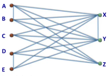
graph is a natural abstraction to model relationships in data, and massive graphs are ubiquitous in applica-tions. Massive graphs have been widely used in modeling real world scenarios such as social networks (e.g., [1], [2]), information retrieval from the web (e.g., [3]), citation net-works (e.g., [4]) and physical simulation and modeling (e.g., [5]). Finding patterns and insights from such data can often be reduced to mining substructures from massive graphs. We consider scalable methods for discovering densely con-nected subgraphs within a large graph. Mining dense sub-structures such as cliques, cliques, bicliques, quasi-bicliques etc. is an important and widely studied research area (see [6], [7], [8], [9]).We focus on a fundamental dense substructure called a biclique. A biclique in an undirected graph G¼ ðV; EÞ is a pair of subsets of verticesLV andRV such that (1)L andRare disjoint and (2) there is an edgeðu; vÞ 2Efor every u2Landv2R. For instance, consider the following graph relevant to an online social network, where there are two types of vertices, users and webpages. There is an edge between a user and a webpage if the user “likes” the web-page on the social network. A biclique in this graph consists of a set of usersUand a set of webpagesW such that every user inUhas liked every page inW. Uncovering such a bicli-que yields a set of users who share a common interest, and is valuable for understanding and predicting the actions of users on this social network. Usually, it is useful to identify maximal bicliques in a graph, which are those bicliques that
are not contained within any other larger bicliques. See Fig. 1 for an example.We consider the problem of enumerating all maxi-mal bicliques from a graph (henceforth referred to as MBE).
Many applications in mining data from the web and online social networks have relied on biclique enumeration on an appropriately defined graph. [10] considered the “click-through” graph for the analysis of web search queries. This graph has two types of vertices, web search queries and web pages. There is an edge from a search query to every page that a user has clicked in response to the search query. MBE was used in clustering queries using the click through graph. MBE has been used by [11] in social network analysis, in detection of communities in social net-works and the web by [12], [13], and in finding antagonistic communities in trust-distrust networks by [14].
In bioinformatics, MBE has been used in constructing the phylogenetic tree of life (see [15], [16], [17], [18]), in discov-ery and analysis of structure in protein-protein interaction networks (see [19], [20]), analysis of gene-phenotype rela-tionships by [21], prediction of miRNA regulatory modules as described by [22], modeling of hot spots at protein inter-faces by [23], and in the analysis of relationships between genotypes, lifestyles, and diseases by [24]. In other contexts, MBE has been used in Learning Context Free Grammars ([25]), finding correlations in databases ([26]), data compres-sion ([27]), role mining in role based access control ([28]), and process operation scheduling ([29]).
However, current state of the art methods for MBE have not been shown to scale to large graphs and have the following drawbacks. First, most methods are sequen-tial algorithms that are unable to use the power of multiple processors; there is very little work on parallel methods for MBE. For handling large graphs, it is impera-tive to have methods that can process a graph in parallel. Next, they have been evaluated only on relatively small graphs with a few thousand vertices and a few thousand
The authors are with the Department of Electrical and Computer Engineering, Iowa State University, Ames, IA 50011.
E-mail: {arko, snt}@iastate.edu.
Manuscript received 13 June 2015; revised 16 Nov. 2015; accepted 25 Jan. 2016. Date of publication 3 Feb. 2016; date of current version 6 Oct. 2017. For information on obtaining reprints of this article, please send e-mail to: [email protected], and reference the Digital Object Identifier below.
Digital Object Identifier no. 10.1109/TSC.2016.2523997
1939-1374ß2016 IEEE. Personal use is permitted, but republication/redistribution requires IEEE permission. See http://www.ieee.org/publications_standards/publications/rights/index.html for more information.
bicliques. For instance, the popular “consensus” method for biclique enumeration by [6] presents experimental data only on random graphs of a low density with up to 2,000 vertices and a few thousand maximal cliques. Other works such as [30], [31] are similar.1
Our goal is to design a parallel method that can enumer-ate maximal bicliques in large graphs, with millions of edges and tens of millions of maximal bicliques, and which can scale with the number of processors.
1.1 Contributions
We present a parallel algorithm for MBE. At a high level, our algorithm clusters the input graph into overlapping subgraphs that are typically much smaller than the input graph, and processes these subgraphs using different paral-lel tasks. For the above cluster generation approach to be effective on large graphs, we needed to solve two problems. The first problem is the overlap in work within different tasks. For biclique enumeration, it is usually not possible to assign disjoint subgraphs to different tasks, and subgraphs assigned to different tasks will overlap, sometimes signifi-cantly. The challenge is to ensure that work done in different tasks overlap as little as possible with each other. We accom-plish this through a careful partitioning of the search space so that even if different tasks are processing overlapping sub-graphs, they still explore disjoint portions of the search space.
The second problem is load balancing among different tasks. With a graph analysis task such as biclique enumera-tion, the complexities of different subgraphs vary signifi-cantly, roughly depending on the density of edges in the subgraph. With a naive assignment of subgraphs to tasks, this will lead to a case where most tasks finish quickly, while a few take a long time, leading to a poor parallel performance. We present a solution to keep the load more balanced, using an ordering of vertices that reduces enumeration load on sub-graphs that are dense, and increases the load on subsub-graphs that are sparse, leading to a better load balance overall. We present two different ordering techniques to achieve this load balance, one based on the size of the neighborhood of the vertex (Algorithm CD1) and the other based on the size of the 2-neighborhood of the vertex (Algorithm CD2).
We provide a theoretical analysis of our algorithms, including proofs of correctness and analysis of computation and communication. Significantly, we show that our
parallel algorithms arework-optimal, i.e., the total computa-tion cost across all processors is the same as that of a sequential algorithm for MBE.
We also consider the related problem of generating only large maximal bicliques, which have at least a certain number of vertices. Our parallel algorithms can be easily adapted to this case, using appropriate changes to underly-ing sequential algorithms.
We also considered another approach to parallel MBE, using a direct parallelization of the “consensus” algo-rithm due to [6], which is probably the most commonly used sequential algorithm for MBE. We found that this method (i.e., parallelization of the consensus algorithm) takes substantially greater runtime than our clustering based method.
We design our algorithms for the MapReduce framework ([32], [33]) and implement it using Hadoop MapReduce. We present detailed experimental results on real-world and synthetic graphs. Overall, the cluster generation approach using a sequential algorithm based on depth-first-search (DFS), when combined with our pruning and load balanc-ing optimizations, performs the best on large graphs, and provides speedups of an order of magnitude over simple approaches to parallelization. This algorithm can process graphs with millions of edges and tens of millions of maxi-mal bicliques, and can scale out with the cluster size. To our knowledge, these are the largest reported graph instances where bicliques have been successfully enumerated.
1.2 Prior and Related Work
There are two general approaches to sequential algorithms for MBE, the “consensus” method due to [6], and methods based on recursive depth-first-search combined with branch-and-bound (see [30], [31], [34]).
The consensus method ([6]) is a very popular iterative algorithm for MBE. In this method, the algorithm starts off with a set of simple maximal bicliques and then expands to the set of all maximal bicliques through a sequence of repeated cross-products, as we explain in the following sections. We developed a direct parallelization of the con-sensus algorithm, but we found that this method performs poorly compared with our cluster generation approach; details are presented in subsequent sections.
Among the DFS based approaches, [30] presents an approach based on a connection with mining closed pat-terns in a transactional database and [31] present a more direct algorithm based on depth first search. Our parallel algorithm uses a sequential algorithm for processing bicli-ques within each task, and we considered both the consensus and the DFS based algorithms; the DFS-based algorithms ran faster overall, and it was easier to optimize the DFS based methods.
Another approach to MBE is through a reduction to the problem of enumerating maximal cliques, as described by [35]. Given a graphGon which we need to enumerate maximal bicliques, a new graph G0 is derived such that through enumerating maximal cliques inG0using an algo-rithm such as by [36], [37], it is possible to derive the maxi-mal bicliques inG. However, this approach is not practical for large graphs since in going fromGtoG0, the number of edges in the graph increases significantly.
Fig. 1. Maximal bicliques.
1. In our experiments, we observed that the consensus method and the other current methods are unable to process our input graphs in a reasonable time.
Parallel algorithms for maximal clique enumeration have been proposed by [38], [39]. Like our method, these also per-form optimizations in the depth first search paths to reduce redundancy. However, these optimizations are specific to the algorithm used and are different from the ones that we use. Note that the maximal clique is a structure that is more “local” than a maximal biclique in the sense that a maximal clique is present within the 1-neighborhood of a vertex in a graph while a maximal biclique goes beyond the 1-neigh-borhood but is contained in a 2-neigh1-neigh-borhood of a vertex. Hence, the difficulty of obtaining an effective parallelization of MBE is higher than that of Maximal Clique Enumeration.
Makino and Uno [40] describe methods to enumerate all maximal bicliques in abipartite graph, with the delay betw-een outputting two bicliques bounded by a polynomial in the maximum degree of the graph. Zhang et al. [41] describe a branch-and-bound algorithm for the same problem. How-ever, these approaches do not work for general graphs, as we consider here.
There is a variant of MBE where we only seek induced maximal bicliques in a graph. An induced maximal biclique is a maximal biclique which is also an induced subgraph. A maximal bicliquehL; Riin graphGis an induced maximal biclique if LandRare themselves independent sets inG. We consider the non-induced version, where edges are allowed in the graph between two vertices that are both in L, or both inR(such edges are of course, not a part of the biclique). The set of maximal bicliques that we output will also contain the set of induced maximal bicliques, which can be obtained by post-processing the output of our algo-rithm. Note that for a bipartite graph, every maximal bicli-que is also an induced maximal biclibicli-que. Algorithms for Induced MBE include work by [42], [43], and [44].
To our knowledge, the only prior work on parallel algorithms for MBE is by [45]. However, this work does not explore aspects of load balancing and total work such as we do. Moreover, their evaluations are not for large graphs; the largest graph they consider has 500 vertices and about 9,000 edges. They do not present any provable properties of their algorithm. Also, their work represents the graph as an adjacency matrix in the memory, whereas we use adjacency list, which takes lesser space and is more practical for large graphs.
MBE is related to, but different from the problem of find-ing the largest sized biclique within a graph (maximum biclique). There are a few variants of the maximum biclique problem, including maximum edge biclique, which seeks the biclique in the graph with the largest number of edges, and maximum vertex biclique, which seeks a biclique with the largest number of edges; for further details and variants, see work by [46]. MBE is harder than finding a maximum biclique, since it enumerates all maximal bicliques, includ-ing all maximum bicliques.
2
P
RELIMINARIESWe present a precise problem definition and briefly review the MapReduce parallel programming model.
2.1 Problem Definition
We consider a simple undirected graphG¼ ðV; EÞwithout self-loops or multiple edges, whereV is the set of all vertices
andE is the set of all edges of the graph. Letn¼j jV and m¼j jE. Graph H¼ ðV1; E1Þ is said to be a sub-graph of
graphGifV1V andE1E.H is known as an induced
subgraph ifE1consists of all edges of Gthat connect two
vertices inV1. For vertexu2V, lethðuÞdenote the vertices
adjacent toS u. For a set of vertices UV, let hðUÞ ¼
u2UhðuÞ. For vertexu2V andk > 0, lethkðuÞdenote all
vertices that can be reached fromuinkhops. ForUV, let
hkðUÞ ¼ S
u2UhkðuÞ. We callhkðUÞas thek-neighborhood of
U. For a set of verticesUV, letGðUÞ ¼Tu2UhðuÞ.
A biclique B¼ hL; Ri is a subgraph of G containing two non-empty and disjoint vertex sets,LandRsuch that for any two vertices u2L and v2R, there is an edge
ðu; vÞ 2E. A bicliqueM¼ hL; RiinGis said to be a maxi-mal biclique if there is no other biclique M0¼ hL0; R0i 6¼
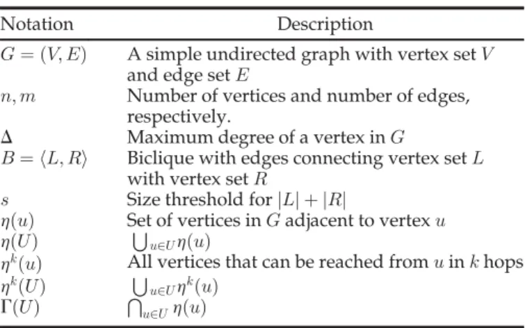
hL; Risuch that LL0 andRR0. The Maximal Biclique Enumeration Problem (MBE) is to enumerate all maximal bicliques in G. Table 1 summarizes the notation used in the paper.
2.2 Sequential Algorithms
We describe the two general approaches to sequential algo-rithms for MBE that we consider, one based on depth first search (see [31]) and another based on a “consensus algo-rithm” (see [6]).
2.2.1 Sequential DFS Algorithm
The basic sequential depth first approach that we use is described in Algorithm 1, based on work by [31]. It attempts to expand an existing maximal biclique into a larger one by including additional vertices that qualify, and declares a biclique as maximal if it cannot be expanded any further. The algorithm takes the following inputs: (1) the graph G¼ ðV; EÞ, (2) the current vertex set being processed, X, (3)T, the tail vertices ofX, i.e., all vertices that come afterX in lexicographical ordering and (4) s, the minimum size threshold below which a maximal biclique is not enumer-ated.scan be set to1so as to enumerate all maximal bicli-ques in the input graph. However, we can setsto a larger value to enumerate only large maximal bicliques such that forB¼ hL; Ri, we havej j L sandj j R s. The size thresh-oldsis provided as user input. The other inputs are initial-ized as follows:X¼?,T ¼V.
TABLE 1 Summary of Notation
Notation Description
G¼ ðV; EÞ A simple undirected graph with vertex setV and edge setE
n; m Number of vertices and number of edges, respectively.
D Maximum degree of a vertex inG
B¼ hL; Ri Biclique with edges connecting vertex setL with vertex setR
s Size threshold forjLj þ jRj
hðuÞ Set of vertices inGadjacent to vertexu hðUÞ Su2UhðuÞ
hkðuÞ All vertices that can be reached fromuinkhops
hkðUÞ S
u2UhkðuÞ
Algorithm 1.MineLMBC(G,X,T,s) 1 for all thevertexv2Tdo
2 ifjGðX[ fvgÞj < sthen 3 T Tn fvg
4 ifj j þX j jT < sthen 5 return
6 Sort vertices inTas per ascending order ofjhðX[ fvgÞj; 7 for all thevertexv2Tdo
8 T Tn fvg 9 ifjX[ fvgj þj j T sthen 10 N GðX[ fvgÞ 11 Y GðNÞ 12 BicliqueB < Y; N > 13 ifðYn ðX[ fvgÞÞ Tthen 14 ifj j Y sthen
15 EmitBas a maximal biclique 16 MineLMBC(G,Y,TnY,s)
The algorithm recursively searches for maximal bicliques. It increases the size ofXby recursively adding vertices from the tail setT, and pruning away those vertices fromTwhich cannot be added to X to expand the biclique. From the expanded X, the algorithm outputs the maximal biclique <GðGðXÞÞ;GðXÞ>. The algorithm is shown [31] to have computational complexity ofOðnDNÞ, wherenis the num-ber of vertices in the graph,Dis the maximum vertex degree andNis the number of maximal bicliques emitted.
2.2.2 Consensus Algorithm
Alexe et al. [6] present an iterative approach to MBE. This algorithm starts off with a set of simple “seed” bicliques. In each iteration, it performs a “consensus” operation, which involves performing a cross-product on the set of current candidates bicliques with the seed bicliques, to generate a new set of candidates, and the process continues until the set of candidates does not change anymore. After each stage, the newly found bicliques can be expanded to find new maximal bicliques. After each step, the duplicate maxi-mal bicliques can be dropped. It is proved that these algo-rithms exactly enumerate the set of maximal bicliques in the input graph. Algorithm 2 shows the sequential consensus Algorithm. For further details, we refer the reader to [6].
The consensus approach has a good theoretical guaran-tee, since its runtime depends on the number of maximal cliques that are output. In particular, the runtime of the MICA version of the algorithm is proved to be bounded by O nð 3NÞ where n is the number of vertices and N total number of maximal bicliques inG. The consensus algorithm has been found to be adequate for many applications and is quite popular.
2.3 Parallel Processing Framework
MapReduce(see [32], [33]) is a popular framework for proc-essing large data sets on a cluster of commodity hardware. A MapReduce program is written through specifying map and reduce functions. The map function takes as input a key-value pairhk; viand emits zero, one, or more new key-value pairshk0; v0i. All tuples with the same value of the key are grouped together and passed to a reduce function, which processes a key k and all values associated with k,
and outputs a final list of key-value pairs. The outputs of one MapReduce round can be the input to the next round. For further details and examples of use, see [32], [33], [47]. We used Hadoop, an open source implementation of Map-Reduce ([48]). Hadoop is built on top of a distributed file system HDFS ([49]). While we evaluated an implementation on top of MapReduce, the idea in our parallel algorithm is more generally applicable and can easily be adapted to other frameworks such as Pregel ([50]) and Spark ([51]). Algorithm 2.Sequential Consensus Algorithm
1 Load GraphG¼ ðV; EÞ
2 R Collection of all Stars inG//Biclique formed by a vertex and its neighbors
3 S ?
4 for all theb2Rdo 5 m Extendb 6 S S[m
7 O S; //Add seed set to the output
8 P S; //Initialize set PREV with SEED
9 repeat
10 T Consensus between all maximal bicliques inS and P;
11 C ?;
12 for all theb2Tdo 13 m Extend bicliqueb 14 ifmis not a duplicatethen
15 C C[m
16 O O[C
17 P C
18 untilNis Empty
3
P
ARALLELA
LGORITHMS FORMBE
We describe our parallel algorithms for MBE, and give an outline of how these are implemented using MapReduce. We first present a basic cluster generation approach,which can be used with any sequential algorithm for MBE, followed by enhancements to the basic cluster generation approach.
3.1 Basic Cluster Generation Approach
For eachv2V, let subgraph (cluster)CðvÞbe defined as the induced subgraph on all vertices inh2ðvÞ. We first note the following.
Lemma 1.For any bicliqueBinGand a vertexvinB,Bis max-imal inGif and only ifBis maximal inCðvÞ.
Proof.SupposeBis maximal inG. Then we first note thatB is a subgraph of CðvÞ. To see this, suppose that B¼
hL; Ri, and without loss of generality, suppose v2L. Then each vertex inR is in hðvÞ, and must be inCðvÞ. Similarly, each vertex in L is in h2ðvÞ, and must be in CðvÞ. Since CðvÞ is a vertex-induced subgraph, it must contain all edges as well as the vertices of the bicliqueB. Next we show B must be a maximal biclique in CðvÞ. Suppose not, andBwas contained in another bicliqueB0 inCðvÞ. SinceB0is also present inG, this implies thatB is not maximal inG, which is a contradiction.
Consider a biclique M¼ hL; Ri that is maximal in CðvÞ, and supposev2L. We show thatM is a maximal biclique in G. Clearly, M is present in G, so it only
remains to be proved thatM is maximal inG. Suppose not, and there was a bicliqueM0¼ hL0; R0iinGsuch that L0L and R0R, and M6¼M0. We note that v2L0, and hence every vertex in R0 and L0 are contained in
h2ðvÞ. Hence, every vertex inM0is contained inCðvÞ, and sinceCðvÞ is a vertex-induced subgraph, every edge of M0is also contained inCðvÞ. This implies thatMis not a maximal biclique inCðvÞ, which is a contradiction. tu
3.2 Algorithm CDFS – Suppressing Duplicates
With the above observation, a basic parallel algorithm for MBE first constructs the different clusters fCðvÞjv2Vg, and then enumerates the maximal bicliques in the dif-ferent clusters in parallel, using any sequential algorit-hm for MBE for enumerating the bicliques within each cluster.
While each maximal biclique inGis indeed enumerated by the above approach, the same biclique may be enumer-ated multiple times. To suppress duplicates, the following strategy is used: a maximal bicliqueBarising from cluster CðvÞis emitted only ifvis the smallest vertex inBaccording to a lexicographic total order on the vertices. The basic clus-ter generation framework is generic and can be used with any sequential algorithm for MBE. We have used a variant of the DFS-based sequential algorithm due to [31], as well as the sequential consensus algorithm due to [6]. We call the above basic clustering algorithm using DFS-based sequen-tial algorithm as “CDFS”.
Observation 1.Algorithm CDFS enumerates every maximal biclique in graphG¼ ðV; EÞexactly once.
There are two significant problems with the CDFS algo-rithm described above. First is redundant work. Although each maximal biclique inG is emitted only once, through suppressing duplicate output, it will still be generated mul-tiple times, in different clusters. This redundant work sig-nificantly adds to the runtime of the algorithm. Second is an uneven distribution of loadamong different subproblems. The load on subproblemCðvÞdepends on two factors, the com-plexity of clusterCðvÞ(i.e., the number and size of maximal bicliques withinCðvÞ) and the position ofvin the total order of the vertices. The earliervappears in the total order, the greater is the likelihood that a maximum biclique in CðvÞ has vhas its smallest vertex, and hence the greater is the responsibility for emitting bicliques that are maximal within CðvÞ. A lexicographic ordering of the vertices will lead to a significantly increased workload for clustersCðvÞ where v appears early in the total order and a correspondingly low workload for clustersCðvÞwherevoccurs earlier in the total order.
3.3 Algorithm CD0 – Reducing Redundant Work
In order to reduce redundant work done at different clus-ters, we begin with the basic cluster generation approach and modify the sequential DFS algorithm for MBE that is executed at each reducer. We first observe that in cluster CðvÞ, the only maximal bicliques that matter are those with vas the smallest vertex; the remaining maximal bicliques in CðvÞ will not be emitted by this reducer, and need not be searched for here. We use this to prune the search space of
the sequential DFS algorithm used at the reducer. The algo-rithm at the reducer is presented in Algoalgo-rithms 7 and 8.
The above algorithm, the “optimized DFS clustering algorithm”, or “CD0” for short, is described in Algorithm 3. This takes two rounds of MapReduce. The first round, described in Algorithms 4 (map) and 5 (reduce), is responsi-ble for generating the 1-neighborhood for each vertex. The second round, described in Algorithms 6 (map) and 7 (reduce) first constructs the clustersCðvÞand runs the opti-mized sequential DFS algorithm at the reducer to enumer-ate local maximal bicliques. We assume that the graph is presented as a file in HDFS organized as a list of edges with each line in the file containing one edge. The flow of execu-tion of this Algorithm is described in Fig. 2.
All search paths in the algorithm which lead to a maxi-mal biclique having a vertex less thanvcan be safely pruned away. Hence, before starting the DFS, we prune away all vertices in the Tail set that are less thanv, as described in Algorithm 7. Also, in DFS Algorithm 8, we prune the search path in Line 12 if the generated neighborhood contains a vertex less thanv– maximal bicliques along this search path will not havevas the smallest vertex. Finally in Line 19 of Algorithm 8, we emit a maximal biclique only if the smallest vertex is the same as the key of the reducer in Algorithm 7. Algorithm 3.Algorithm CD0
Input:Edge List ofG¼ ðV; EÞ 1 Execution Flow as per Fig. 2
Algorithm 4.Algorithm CD0 Round One – Map Input:Edgeðx; yÞ
1 //Generate Adjacency List for vertices x and y
2 Emit (key x,value y) 3 Emit (key y,value x)
Algorithm 5.Algorithm CD0 Round One – Reduce Input:key¼v,value¼ fv1; v2; ; vdg
1 //Generate Adjacency List for vertex v
2 N ?;
3 for all theval2valuedo 4 N N[val;
5 //Add the neighbors of key to N
6 Emit (key v,value N)
Algorithm 6.Algorithm CD0 Round Two – Map Input:key¼v,value¼N
1 //Create Two Neighborhood for vertex v
2 Emit (key v,value N); 3 for all they2Ndo
4 Emit (key y,value hv; Ni) Fig. 2. Execution flow for Algorithm 3 (CD0).
Algorithm 7.Algorithm CD0 Round Two – Reduce Input:key¼v,value¼ fhðvÞ;hðv1Þ;hðv2Þ;. . .;hðvdÞg
1 //Create Two Neighborhood for vertex v from the values received
2 G0¼ ðV0; E0Þ Induced subgraph onh2ðvÞ 3 X key
4 T V0n fkeyg
5 for all thevertext2Tdo 6 ift < keythen 7 T Tn ftg
8 O Mapping between vertex identifiers and their lexico-graphical ordering;
9 Algorithm 8 (G0,X,T,key,s,O)
Algorithm 8.CD0_Sequential(G0,X,T,key,s,O) Input:G0,X,T,key,s,O
1 //The sequential Algorithm to be run indepen-dently on each cluster for the parallel Algorithm 2 ifX = {key}then 3 N GðXÞ//Same asGðkeyÞ 4 Y GðNÞ 5 ifY ¼Xthen 6 BicliqueB < Y; N > 7 ifj j Y s^j j N sthen
8 vs Smallest vertex inBas per the ordering inO
9 ifvs¼keythen
10 //Maximal biclique found
11 Emit (key ?,value B) 12 else
13 return
14 for all thevertexv2Tdo 15 ifjGðX[ fvgÞj < sthen 16 T Tn fvg
17 ifj j þX j jT < sthen 18 return
19 Sort vertices inTas per ascending order ofjGðX[ fvgÞj 20 for all thevertexv2Tdo
21 T Tn fvg
22 ifjX[ fvgj þj j T sthen 23 N GðX[ fvgÞ 24 Y GðNÞ
25 ifY contains vertices smaller thankeyas per the ordering in Othen
26 continue
27 BicliqueB < Y; N > 28 ifðYn ðX[ fvgÞÞ Tthen 29 ifj j Y sthen
30 vs Smallest vertex inBas per the ordering inO
31 ifvs¼keythen
32 //Maximal biclique found
33 Emit (key ?,value B) 34 CD0_Sequential(G0,Y,TnY,key,s,O)
Since Algorithm 8 is a pruned version of the sequential DFS Algorithm 1, the computation complexity of Algo-rithm 8 isO nð cDvNðvÞÞ, wherenc is the number of
verti-ces inCðvÞ,Dvis the maximum degree of all vertices inCðvÞ
and NðvÞ is the number of maximal bicliques in G,
containingv. SinceDvcannot be greater thannc, we can also
write the computation complexity asO nð c2NðvÞÞ.
Lemma 2.Algorithm 3 generates all maximal bicliques in a graph. Proof.The correctness of this Lemma can be proved from Lemma 1. Algorithm 3 generates the 2-neighborhood induced sub–graph of each vertex inG. It then runs the optimized sequential DFS algorithm that enumerates for each C(v), all the maximal bicliques where v is the
small-est vertex. tu
Lemma 3. The total work done by Algorithm 3 is equal to the work done by the sequential DFS Algorithm 1.
Proof.Algorithm 3 calls Algorithm 8 once for each vertex v2V for the input graph G¼ ðV; EÞ. Thus there is one instance of Algorithm 8 created in parallel for each vertex vwith inputCðvÞ. Before we prove this, note that the the sequential DFS Algorithm 1 can be represented as a tree as follows. Let each recursive call to the method be a node in the tree. Let the value of the node be the set of vertices in the working setXin Algorithm 1. Each recur-sive call establishes a parent–child relationship where the calling instance of the method becomes the parent. Now to prove this lemma, we show that the work done by parallel instance of Algorithm 8 for vertexvis same as work done by the subtree of the sequential Algorithm 1 that starts withX¼v.
Consider the root of the search tree for the sequential Algorithm 1. At the root the working setXis ?. Let us consider the root to be depth0. Let us assume some pre-defined ordering strategy of the tail set “T”. Also, let us label the vertices v1. . .vn following the ordering. Then
for each vertex, v2V, we have a branch that comes out of the root. Thus for depth 1, we have ðX1 1,
T1 V n f1gÞ,ðX2 2,T2 V n f1;2gÞand so on. Thus
for each v2V, we have ðXv v, T1 V n f1;2;. . .;
v1gÞ. Hence for depth1, we have the above mentioned V
j jcalls.
Now we show that each such branch corresponds to the instance of the parallel Algorithm 8 such that the reducerkey¼v.
To prove this, we note the call made to Algorithm 8 with key v. Algorithm 8 is called with X¼key and
8t2T, t > v. Thus we prune T such that T V n f1;
2;. . .; v1g. This call is same as the branch of the search tree of Algorithm 1 that starts withkey. The input graph to the parallel algorithm is different from the sequential one. However, from Lemma 1, this doesn’t make a differ-ence to the output of the parallel Algorithm.
Now, Algorithm 8 is different from Algorithm 1 in Lines 1-12 of Algorithm 8. However, we note that these lines simulate the call made in Algorithm 8 withX¼v. All further recursive calls that follow are identical in both Algorithms 8 and 1. tu
3.4 Algorithms CD1 and CD2 – Improving
Load Balance
In Algorithm CD0, vertices were ordered using a lexico-graphic ordering, which is agnostic of the properties of the clusterCðvÞ. The way the optimized DFS algorithm works, the enumeration load on a cluster CðvÞ depends on the
number of maximal bicliques within this cluster as well as the position of v within the total order. The earlier that v is in the total order, the greater is the load on the reducer handlingCðvÞ.
For improving load balance, our idea is to adjust the position of vertexvin the total order according to the prop-erties of its clusterCðvÞ. Intuitively, the more complex clus-terCðvÞis (i.e., more and larger the maximal bicliques), the higher should be position ofvin the total order, so that the burden on the reducer handlingCðvÞis reduced. While it is hard to compute (or even accurately estimate) the number of maximal bicliques inCðvÞ, we consider two properties of vertexvthat are simpler to estimate, to determine the rela-tive ordering of vin the total order: (1) Size of 1-neighbor-hood ofv(Degree), and (2) Size of 2-neighborhood ofv.
Intuitively, we can expect that vertices with higher degrees are potentially part of a denser part of the graph and are contained within a greater number of maximal bicli-ques. The size of the 2-neighborhood is also the number of vertices in CðvÞ and may provide a better estimate of the complexity of handlingCðvÞ, but this is more expensive to compute than the size of the 1-neighborhood of the vertex.
The discussion below is generic and holds for both approaches to load balancing. To run the load balanced ver-sion of DFS, the reducer running the sequential algorithm must now have the following information for the vertex (key of the reducer) : (1) 2-neighborhood induced subgraph, and (2) vertex property for every vertex in the 2-neighbor-hood induced subgraph, where “vertex property” is the property used to determine the total order, be it the degree of the vertex or the size of the 2-neighborhood. The second piece of information is required to compute the new vertex ordering. However, the reducer of the second round does not have this information for every vertex in CðvÞ, and a third round of MapReduce is needed to disseminate this information among all reducers. We call the Algorithm using the size of 1–neighborhood of a vertexvas the heuris-tic as CD1 and the one using the size of 2–neighborhood as CD2. The high level overviews of Algorithms CD1 and CD2 are described in Fig. 3. Following similar arguments as pre-sented for Algorithm 8, Algorithms CD1/CD2 also has com-putation complexity ofO nð cDvNðvÞÞ ¼O nð c2NðvÞÞ.
Lemma 4.The total work done by parallel Algorithm 9 is equal to the work done by the sequential DFS Algorithm 1.
Proof. Note that the only difference between Algorithm 9 and Algorithm 3 is how they order the vertices. Algo-rithm 3 uses lexicographical ordering of vertices where as Algorithm 9 uses either degree or size of 2–neighbor-hood. Hence, the proof follows from the proof of Lemma 3. This is because, the proof of Lemma 3 makes no assumption on the strategy used to order the vertices
in the graph. tu
Algorithm 9.Algorithms CD1 and CD2 Input:Edge List ofG¼ ðV; EÞ
1 Execution Flow as per Fig. 3
3.5 Communication Complexity
We consider the communication complexity of Algorithms CD0, CD1 and CD2. For input graph G¼ðV; EÞ, recall n¼j jV andm¼j jE. LetDdenote the largest degree among all vertices in the graph. Also, letbdenote the output size, defined as the sum of the numbers of edges of all enumer-ated maximal bicliques.
Definition 1.The communication complexity of a MapReduce algorithm is defined as the sum of the total number of bytes emitted by all mappers and the total number of bytes emitted by all the reducers across all rounds.
Lemma 5.The communication complexity of Algorithm CD0 is O mð DþbÞ.
Proof.Algorithm CD0 has two rounds of MapReduce. In the first round the Map method (Algorithm 4) emits each edge twice, resulting in a communication complexity of O mð Þ. Similarly, the reducer (Algorithm 5), emits each adjacency list once. This also results in a communication complexity of O mð Þ. Hence total communication com-plexity of the first round isO mð Þ.
Now let us consider the second round of MapReduce. The total communication between the Map and Reduce methods (Algorithms 6 and 7 respectively) can be com-puted by analyzing how much data is received by all Reducers. Each reducer receives the adjacency list of all the neighbors of the key. Letdibe the degree of vertexvi,
forvi2V,i¼1; ::; n. The adjacency list of vertexvis sent
to all vertices in that list. The size of adjacency list isdi.
This list is sent todivertices. Thus communication
com-plexity for vertexvibecomesdi2. Total communication is
thus Pni¼1di2¼O D
Pn i¼1di
. Since Pni¼1di¼2m, the
total communication becomesO mð DÞ. The output from the final Reducer (Algorithm 7) is the collection of all max-imal bicliques and hence the resulting communication cost isOð Þb. Combining two rounds, total communication complexity becomesO mð þmDþbÞ.¼O mð DþbÞ. tu Lemma 6.The communication complexity of Algorithm CD1 as
well as CD2 isO mð DþbÞ.
Proof.First, note that both Algorithms CD1 and CD2 have the same communication complexity and observe that the first round uses the same Map and Reduce methods as CD0. Thus communication for Round 1 is O mð Þ. Again, note that Map method for Round 2 is same as CD0 and hence by Lemma 5, communication for Round 2 isO mð DÞ.
The Reducer (Algorithm 10) of Round 2 sends the vertex property information to all its 2–neighbors. Thus every reducer receives information about all of its 2–neighbors. This makes the total output size of Reducer to beO mð DÞ. The Map method of Round 3 (Algorithm 11) sends out the 2–neighborhood information as well as the vertex informa-tion to all vertices in 2–neighborhood. Thus communica-tion cost becomes O mð DÞ. The Reducer (Algorithm 12) emits all maximal bicliques and hence the resulting com-munication cost isOð Þb. Thus total communication cost for Algorithms CD1 and CD2 is isO mð DþbÞ. tu Algorithm 10.Algorithms CD1 and CD2 Round
Two – Reduce
Input:key¼v,value¼ fhðvÞ;hðv1Þ;hðv2Þ; ;hðvdÞg
1 // Send vertex property of vertex v to required nodes
2 S 2-neighbors ofv
3 N Compute neighborhood ofvfromS 4 //Need to pass neighborhood for Round 3
5 Emit (key v,value N)
6 //Need to send vertex property to all 2–neighbors
7 p Value of vertex property ofvfromS 8 for all theverticess2Sdo
9 Emit(key s,value ½v; p)
Algorithm 11.Algorithms CD1 and CD2 Round Three – Map
Input:key¼v; value¼NORkey¼s; value¼v; p
1 // Create Two Neighborhood along with vertex property
2 ifkey¼vthen
3 Emit (key v,value N) 4 for all they2Ndo
5 Emit (key y,value hv; Ni) 6 else
7 Emit (key s,value ½v; p)
Algorithm 12.Algorithms CD1 and CD2 Round Three – Reduce
Input:key¼v,value¼{h2ðvÞalong with vertex properties} 1 // Create Two Neighborhood along with vertex
property
2 G0¼ ðV0; E0Þ Induced subgraph onh2ðvÞ
3 Map HashMap of vertex and vertex property created from valuerequired to compute the new ordering
4 X key 5 T V0n fkeyg
6 for all thevertext2Tdo
7 ift < keyin the new orderingthen 8 T Tn ftg
9 Algorithm 8(G0,X,T,key,s,Map)
4
P
ARALLELC
ONSENSUSWe describe another approach, a direct parallelization of the consensus sequential algorithm of [6]. The motivation for trying this approach was that the cluster generation
approach requires each cluster CðvÞ to have the entire 2-neighborhood ofv, whereas the parallel consensus appro-ach does not require the generation of 2-neighborhood of vertices. Note that although this algorithm takes less mem-ory per reducer than the cluster generation algorithm, we found the parallel consensus algorithm to be much slower, overall, than Algorithms CD1/CD2. We present the parallel consensus algorithm in this section.
Unlike the parallel DFS algorithm which works on sub-graphs of G, the consensus algorithm is always directly dealing with bicliques within graphG. At a high level, it performs two operations repeatedly (1) a “consensus” oper-ation, which creates new bicliques by considering the combination of existing bicliques, and (2) an “extension” operation, which extends existing bicliques to form new maximal bicliques. There is also a need for eliminating duplicates after each iteration, and also a step needed for detecting convergence, which happens when the set of max-imal bicliques is stable and does not change further.
We developed a parallel version of each of these opera-tions, by performing the consensus, extension and duplicate removal using MapReduce.
Algorithm 13.Parallel Consensus Algorithm – Driver Program
1 Load Graph G = (V, E)
2R Star bicliques from G// Biclique formed by a vertex and its neighbors
3 S Extend all bicliques inRusing MapReduce 4 Eliminate duplicates fromSusing MapReduce 5 O O[S
6 P S 7 repeat
8 T Consensus among all maximal bicliques inSandP using MapReduce
9 C Extend all bicliques inTusing MapReduce 10 Eliminate duplicates fromCusing MapReduce 11 O O[C
12 P C
13 untilNis?
Our Algorithm is described in Algorithm 13. Algo-rithms 14 and 15 (map and reduce) describe the consensus operation using MapReduce. Note that in Algorithm 13, line 8 performs consensus between each pair of biclique in sets S (seed set) and P (set of bicliques from previous round of iteration). To perform consensus between the all bicliques from the sets S and P naively, it would requirej jS $j jP con-sensus operations. However, we reduce the total number of consensus operations using the following observation: If there are no common vertices between two bicliques, in that case the consensus output between the concerned two bicli-ques is the NULL set. This is because the intersection opera-tion in the consensus will result in NULL. This helps us to “group” the bicliques inn¼j jV sets, one for each vertex of the graph. A biclique is a part of the group for vertexv, ifv is contained in the biclique. The map method helps to achieve this by “grouping” all bicliques having a particular vertex in common, thus eliminating the need of doing unnecessary consensus operations. Next we explain the extension operation. To reduce memory requirement, we
required four rounds of MapReduce to perform the exten-sion. The intention of the process is to bring together only those neighborhood information, which is required to extend a biclique. Algorithms 16 and 17 describe the map and reduce algorithms for the first round. Recall that the extension operation requires computation of 2-neighbor-hood of both the left and right set of the vertices in the bicli-que. The first two rounds of MapReduce are used to compute the 1-neighborhood of both the sets and then the same two rounds are run one more time to obtain the 2-neighborhood information. Finally, the algorithm stops when no new maximal bicliques are found after completing an iteration. The Driver Algorithm 13 checks for the same and halts if no new maximal bicliques are found.
Algorithm 14.Parallel Consensus Algorithm – Consen-sus Map
1 for all theisuch thatiis an node in the left set of the bicliqueH do
2 Emitði; HÞ
3 for all thejsuch thatjis an node in the right set of the bicliqueH do
4 Emitðj; HÞ
Algorithm 15.Parallel Consensus Algorithm – Consen-sus Reduce
1 for all thexsuch thatxis a seed biclique containing the keykdo 2 for all theysuch thatyis a biclique from previous round having
the keykdo
3 ifkey =minimum common element of the bicliques x and y
then
4 C Potentially new maximal bicliques from consen-sus ofxandy
5 for all thecinCdo
6 Extend the bicliquecto generate maximal bicliqueH 7 Emitð?; HÞ
Algorithm 16.Parallel Consensus Algorithm – Extension Map
1 B Input biclique 2 ifBisa starthen 3 x Main vertex 4 Emit (x,B)
5 ifdata is from consensus outputthen 6 for all the verticesisuch thatiis inBdo 7 Emit (i,B)
5
E
XPERIMENTALR
ESULTSWe implemented our parallel algorithms on a Hadoop ter, using both real-world and synthetic datasets. The clus-ter has 28 nodes, each with a quad-core AMD Opclus-teron processor with 8 GB of RAM. All programs were written using Java version 1.5.0 with 2 GB of heap space, and the Hadoop version used was 1.2.1.
We implemented the DFS based algorithms CDFS (clus-tering DFS with no optimizations), CD0 (clus(clus-tering DFS with the pruning optimization), CD1 (clustering DFS with
pruning and load balancing using degree), and CD2 (clus-tering DFS with pruning and load balancing using size of 2-neighborhood). Table 2 summarizes the various Depth First Search Algorithms that were compared.
Algorithm 17.Parallel Consensus Algorithm – Extension Reduce
1 S ?
2 for all thevalueforkeydo
3 ifvalueis a neighborhood informationthen 4 N Neighborhood of vertexkey 5 else
6 S S[value
7 for all thebicliquesbinSdo 8 h Hash value of bicliqueb 9 Emit (h,b)
10 Emit (h,N)
We also implemented the sequential DFS algorithm due to [31], and the sequential consensus algorithm (MICA) due to [6]. The sequential algorithms were not implemented on top of Hadoop and hence had no associated Hadoop over-head in their runtime. But on the real-world graphs that we considered, the sequential algorithms did not complete within 12 hours, except for the p2p-Gnutella09 graph. In addi-tion, we implemented the parallel clustering algorithm using the consensus-based sequential algorithm, and we also imple-mented an alternate parallel implementation of the consensus algorithm that was not based on the clustering method.
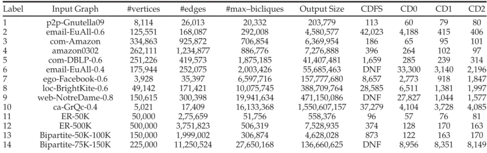
We used both synthetic and real-world graphs. A sum-mary of all the graphs used is shown in Table 3. The real-world graphs were obtained from the SNAP collection of large networks (see [52]) and were drawn from social net-works, collaboration netnet-works, communication netnet-works, product co-purchasing networks, and internet peer-to-peer networks. Some of the real world networks were so large and dense that no algorithm was able to process them. For such graphs, we thinned them down by deleting edges with a certain probability. This makes the graphs less dense, yet preserves some of the structure of the real-world graph. We show the edge deletion probability in the name of the net-work. For example, graph “ca-GrQc-0.4” is obtained from “ca-GrQc” by deleting each edge with probability0:4. Syn-thetic graphs are either random graphs obtained by the Erdos-Renyi model (see [53]), or random bipartite graphs obtained using a similar model. To generate a bipartite graph withn1andn2vertices respectively in the two
parti-tions, we randomly assign an edge between each vertex in TABLE 2
Different Versions of Parallel Algorithms Based on Depth First Search (DFS)
Label Algorithm
CDFS Clustering based on Depth First Search (DFS) CD0 CDFS + Reducing redundant work, without
load balancing
CD1 CDFS + Reducing redundant work + load balancing using degree
CD2 CDFS + Reducing redundant work + load balancing using Size of 2-neighborhood
the left partition to each vertex in the right partition. A ran-dom Erdos-Renyi graph on n vertices is named “ER-hni”, and a random bipartite graph withn1andn2vertices in the
bipartitions is called “Bipartite-hn1i-hn2i”.
We seek to answer the following questions from the experiments: (1) What is the relative performance of the different methods for MBE? (2) How do these methods scale with increasing number of reducers? and (3) How does the runtime depend on the input size and the output size?
Fig. 4 presents a summary of the runtime data for the algorithms in Table 3. All data used for these plots was gen-erated with 100 reducers. The runtime(s) given in Table 3 for various Algorithms were recorded by taking the mean
over five individual runs. The runtime data given for the parallel algorithms include the time required to run all MapReduce rounds including time required to construct 2-neighborhood etc.
5.1 Impact of the Pruning Optimization
From Fig. 4, we can see that the optimizations to basic DFS clustering through eliminating redundant work make a sig-nificant impact to the runtime for all input graphs. For instance, in Fig. 4d, on input graph email-EuAll-0.6 CD0, which incorporates these optimizations, runs10times faster than CDFS, the basic cluster generation approach. Also, we can see from Table 3 that the input graphs email-EuAll-0.4, web-NotreDame-0.8 and Bipartite-75–150K could not be TABLE 3
Properties of the Input Graphs Used, and Runtime (in Seconds) to Enumerate All Maximal Bicliques Using 100 Reducers Label Input Graph #vertices #edges #max–bicliques Output Size CDFS CD0 CD1 CD2
1 p2p-Gnutella09 8,114 26,013 20,332 203,779 113 60 79 80 2 email-EuAll-0.6 125,551 168,087 292,008 4,580,577 42,023 4,188 415 406 3 com-Amazon 334,863 925,872 706,854 6,369,954 186 65 95 101 4 amazon0302 262,111 1,234,877 886,776 7,276,888 396 264 102 97 5 com-DBLP-0.6 251,226 419,573 1,875,185 41,407,481 1,659 285 239 314 6 email-EuAll-0.4 175,944 252,075 2,003,426 55,685,463 DNF 33,300 3,140 2,196 7 ego-Facebook-0.6 3,928 35,397 6,597,716 157,777,680 8,657 2,773 918 1,847 8 loc-BrightKite-0.6 49,142 171,421 10,075,745 388,709,764 28,585 6,511 1,381 1,997 9 web-NotreDame-0.8 150,615 300,398 19,941,634 471,150,086 DNF 27,827 1,044 1,577 10 ca-GrQc-0.4 5,021 17,409 16,133,368 1,550,607,157 37,279 4,104 3,728 4,085 11 ER-50K 50,000 2,75,659 51,756 558,376 96 57 76 81 12 ER-500K 500,000 3,751,823 506,319 7,528,935 374 128 170 163 13 Bipartite-50K-100K 150,000 1,999,002 306,874 4,628,028 873 122 163 170 14 Bipartite-75K-150K 225,000 11,250,524 27,650,168 136,660,625 DNF 8,956 8,351 8,149
DNF means that the algorithm did not finish in 12 hours. The size threshold was set as1to enumerate all maximal bicliques. Runtime includes overhead of all MapReduce rounds including graph clustering, i.e., formation of 2–neighborhood. Graphs 1-10 are real world graphs while the rest are synthetic graphs. We have used random graphs of various sizes between 50 and 500 K vertices, but do not show the details about all synthetic graphs in the table, due to space constraints. All runtimes shown are a mean of five individual runs of the Algorithm.
Fig. 4. Runtime in seconds of parallel algorithms on real and random graphs. If an algorithm failed to complete in 12 hours the result is not shown. All algorithms were run using 100 reducers. All runtimes are a mean of five individual runs of the Algorithm. Runtime includes overhead of all MapRe-duce rounds including graph clustering, i.e., formation of 2–neighborhood.
processed by Algorithm CDFS within 11 hours but could be processed by Algorithm CD0.
We measure the redundant processing that we avoid by using the optimized Algorithm CD0 rather than CDFS. To measure this we count the total number of recursive calls made to the depth first search method by the algorithms. We observe that the number of such recursive calls made by CDFS is an order greater than CD0. For example, for input graph ER-500K, CDFS makes about 16:5 million calls whereas CD0 makes only about 1 million calls. Similar results are obtained for real work input graphs. For exam-ple, for input graph ego-Facebook-0.6, CDFS makes about
133:5 million recursive calls while CD0 makes about only about13:2million. Hence we observe that our optimizations are successful in pruning the search tree by effectively removing redundant search paths.
5.2 Impact of Load Balancing
From Fig. 4, we observe that for graphs on which the algo-rithms do not finish very quickly (within200seconds), load balancing helps significantly. In Fig. 4d, for graph email-EuAll-0.6, the Load Balancing approaches (CD1 and CD2) are10to10:3times faster than CD0, which incorporates the pruning optimization, without load balancing. In Fig. 4b, we note that for input graph web–NotreDame-0.8, CD1 was
26:7 times faster than CD0 and CD2 was about17:6 times faster. We can also observe the improvements in Load Bal-ance from the reducer timings. For input graph email-EuAll-0.4, we observe that for CD0, most reducers finish in a few minutes. A very few took2hours. However, the last two reducers took 4:5 and 9:25 hours. By improving load balance in Algorithms CD1/CD2, we redistribute this work load bringing the parallel runtime of both Algorithms to below one hour.
For most input graphs, the versions optimized through load balancing and pruning (Algorithms CD1 and CD2) worked the best overall, and both these optimizations helped significantly in reducing the runtime.
However, for graphs that completed quickly, load bal-ancing performs slightly slower than Algorithm CD0 (see Fig. 4a). This can be explained by the additional overhead of load balancing (an extra round of MapReduce), which does not payoff unless the work done at the DFS step is significant.
There are two different approaches to load balancing, one based on the vertex degree (Algorithm CD1) and the
other on the size of the 2-neighborhood of the vertex (Algo-rithm CD2).From Fig. 4 we observed that no one approach was consistently better than the other, and the performance of the two were close to each other.For some input graphs, like Email-EuAll-0.4, the 2-neighborhood approach (CD2) fared better than the degree approach (CD1), whereas for some other input graphs like web-NotreDame-0.8, the degree approach fared better.
To better understand the impact of load balancing, we cal-culated the mean and the standard deviation of the run time of each of the 100 reducers for the last round of MapReduce of Algorithms CD0, CD1 and CD2. We present results of this analysis for input graphs loc-BrightKite-0.6 and ego-Face-book-0.6 in Table 4. The load balanced CD1 and CD2 have a much smaller standard deviation for reducer runtimes than CD0.
We observe that random graphs have less variance in degree/size of 2–neighborhood than real world graphs. This leads to approximately balanced load on each node in the cluster, irrespective of how the work is distributed. Hence we don’t get benefit out of the extra overhead involved in CD1 and CD2. Thus for randoms graphs, Algo-rithm CD0 performs better than AlgoAlgo-rithms CD1/CD2.
5.3 Scaling with Number of Reducers
In Fig. 5 we plot the runtime of CD1 and CD2 with increas-ing number of reducers. In Fig. 6, we also plot the speedup, defined as the ratio of the time taken with1reducer to the time taken withrreducers, as a function of the number of reducers r. We observe that the runtime decreases with increasing number of reducers. Both CD1 and CD2 achieves acceptable speedup. For instance for Algorithm CD1 and input graph email-EuAll-0.6, for 5 reducers we get 4:8 speedup while for 80 reducers, we get 49:54 speedup. Similarly, for Algorithm CD2 and input graph email-EuAll-0.6, we achieve speedup of4:9with5reducers and
55:73speedup with 80reducers. This data shows that the algorithms are scalable and may be used with larger clus-ters as well.
TABLE 4
Mean and Standard Deviation Computation of All 100 Reducer Runtimes for Algorithms CD0, CD1 and CD2
loc-BrightKite-0.6 CD0 CD1 CD2 Average 637.27 387.77 393.68 Variance 1,259,680.12 81,447.47 111,443.13 Standard Deviation 1,122.35 285.39 333.83 ego-Facebook-0.6 CD0 CD1 CD2 Average 313.56 245.21 273.43 Variance 203,661.36 29,166.29 108,260.19 Standard Deviation 451.29 170.78 329.03
The analysis is done for the reducer of the last Map Reduce round as it per-forms the actual depth first search.
Fig. 5. Runtime versus number of reducers.
5.4 Relationship to Output Size
We observed the change in runtime of the algorithms with respect to the output size. We define the output size of the problem as the sum of the numbers of edges of all enumer-ated maximal bicliques. Fig. 7 shows the runtime of algo-rithms CD0, CD1, and CD2 as a function of the output size. This data is only constructed for random graphs, where the different graphs considered are generated using the same model, and hence have very similar structure. We observe thatthe runtime increases almost linearly with the output size for all three algorithms CD0, CD1, and CD2.
With real world graphs, this comparison does not seem as appropriate, since the different real worlds graphs have completely different structures; however, we observed that the runtimes of Algorithms CD1 and CD2 are well corre-lated with the output size, even on real world graphs.
5.5 Large Maximal Bicliques
Next, we considered the variant where only large bicliques, whose total number of vertices is at leasts, are required to be emitted. Fig. 8 shows the runtime as the size thresholds varies from 1 to 5. We observe that the runtime decreases significantly as the threshold increases. Also, Algorithms CD1 and CD2 were not able to enumerate all maximal bicli-ques from input graph email-EuAll-0.2 even after12hours. However, with size threshold 5, Algorithm CD1 took less than 6 hours to process this graph while Algorithm CD2 took about3:5hours.
5.6 Consensus versus Depth First Search
Finally we compare the two sequential techniques used in this work. The basic clustering method was used with the
consensus technique and compared with Algorithms CD1 and CD2. Fig. 9 shows the performance of Algorithms CD1 and CD2 against the consensus approach. We note that the cluster generation approach using the consensus technique performed very poorly compared with the DFS based algo-rithm. For example for the input graph p2p-Gnutella09, CD1 and CD2 took 79 and 80 seconds respectively (using 100 reducers). This is in contrast with the implementation of the clustering method using the consensus technique which took1;469seconds (again with 100 reducers). In all instances except for very small input graphs, clustering using consen-sus was6to15times slower than CD1 and CD2 or worse, and in many cases, clustering consensus did not finish within
12hours while CD1 and CD2 finished within1-2hours. We also compared the runtime of the more direct parallel implementation of the consensus technique as described in Algorithm 13. The direct parallel consensus, which uses a different parallelization strategy was13to400times slower than clustering consensus. For example, for input graph ER-500K, Algorithm CD1 finished processing in 170 seconds, whereas Algorithm 13 took over18hours. Further, it could not process the p2p-Gnutella09 input graph within12hours.
6
C
ONCLUSIONMaximal biclique enumeration is a fundamental tool in uncovering dense relationships within graphical data. We presented a scalable parallel method for mining maximal bicliques from a large graph. Our method uses a basic clus-tering framework for parallelizing the enumeration, fol-lowed by two optimizations, one for reducing redundant work, and another for improving load balance. Experimen-tal results using MapReduce show that the algorithms are effective in handling large graphs, and scale with increasing number of reducers. To our knowledge, this is the first work to successfully enumerate bicliques from graphs of this size; previous reported results were mostly sequential methods that worked on much smaller graphs.
The following directions are interesting for exploration (1) How does this approach perform on even larger clusters, and consequently, larger input graphs? What are the bottle-necks here? and (2) Can these be extended to enumerate near-bicliques (quasi-bicliques) from a graph?
A
CKNOWLEDGMENTSThis work was funded in part by the US National Science Foundation through grants 0834743 and 0831903 and is Fig. 7. Runtime versus Output Size for random graphs. All Erdos-Renyi
random graphs were used. Output size of a single maximal biclique is defined as the number of edges in the biclique. The total output size is the sum of the output sizes taken over all the bicliques generated by the algorithm.
Fig. 8. Runtime versus the size threshold for the emitted maximal bicli-ques. All experiments were performed using Algorithm CD1 and with 100 reducers.
Fig. 9. Comparison of the parallel consensus and clustering consensus with Algorithms CD1 and CD2. We observe that the consensus algo-rithm performs poorly in comparison with CD1 and CD2.
partially supported by the HPC equipment purchased thro-ugh NSF MRI grant number CNS 1229081 and NSF CRI grant number 1205413. The views and conclusions contained in this document are those of the author(s) and should not be inter-preted as representing the official policies, either expressed or implied of the US National Science Foundation.
R
EFERENCES[1] A. Mislove, M. Marcon, K. P. Gummadi, P. Druschel, and B. Bhattacharjee, “Measurement and analysis of online social networks,” inProc. 7th ACM SIGCOMM Conf. Internet Meas., 2007, pp. 29–42.
[2] M. E. J. Newman, D. J. Watts, and S. H. Strogatz, “Random graph models of social networks,” Proc. Nat. Acad. Sci. USA, vol. 99, no. Suppl 1, pp. 2566–2572, 2002.
[3] A. Broder, R. Kumar, F. Maghoul, P. Raghavan, S. Rajagopalan, R. Stata, A. Tomkins, and J. Wiener, “Graph structure in the web,”
Comput. Netw., vol. 33, no. 1, pp. 309–320, 2000.
[4] Y. An, J. Janssen, and E. E. Milios, “Characterizing and mining the citation graph of the computer science literature,” Knowl. Inf. Syst., vol. 6, pp. 664–678, 2004.
[5] O. Wodo, S. Tirthapura, S. Chaudhary, and B. Ganapathysubra-manian, “A graph-based formulation for computational character-ization of bulk heterojunction morphology,” Organic Electron., vol. 13, no. 6, pp. 1105–1113, 2012.
[6] G. Alexe, S. Alexe, Y. Crama, S. Foldes, P. L. Hammer, and B. Simeone, “Consensus algorithms for the generation of all maxi-mal bicliques,”Discrete Appl. Math., vol. 145, no. 1, pp. 11–21, 2004. [7] D. Gibson, R. Kumar, and A. Tomkins, “Discovering large dense subgraphs in massive graphs,” inProc. 31st Int. Conf. Very Large Data Bases, 2005, pp. 721–732.
[8] J. Abello, M. G. C. Resende, and S. Sudarsky, “Massive quasi-clique detection,” inProc. 5th Latin Am. Symp. Theoretical Informat., 2002, vol. 2286, pp. 598–612.
[9] K. Sim, J. Li, V. Gopalkrishnan, and G. Liu, “Mining maximal quasi-bicliques to co-cluster stocks and financial ratios for value investment,” inProc. 6th Int. Conf. Data Mining, 2006, pp. 1059– 1063.
[10] J. Yi and F. Maghoul, “Query clustering using click-through graph,” inProc. 18th Int. Conf. World Wide Web, 2009, pp. 1055– 1056.
[11] S. Lehmann, M. Schwartz, and L. K. Hansen, “Biclique communities,”Phys. Rev. E, vol. 78, p. 016108, 2008.
[12] R. Kumar, P. Raghavan, S. Rajagopalan, and A. Tomkins, “Trawling the web for emerging cyber-communities,” Comput. Netw., vol. 31, no. 11, pp. 1481–1493, 1999.
[13] J. E. Rome and R. M. Haralick, “Towards a formal concept analysis approach to exploring communities on the world wide web,” inProc. 3rd Int. Conf. Formal Concept Anal., 2005, vol. 3403, pp. 33–48.
[14] D. Lo, D. Surian, K. Zhang, and E.-P. Lim, “Mining direct antago-nistic communities in explicit trust networks,” inProc. 20th ACM Int. Conf. Inf. Knowl. Manage., 2011, pp. 1013–1018.
[15] A. C. Driskell, C. Ane, J. G. Burleigh, M. M. McMahon, B. C. O’Meara, and M. J. Sanderson, “Prospects for building the tree of life from large sequence databases,”Science, vol. 306, no. 5699, pp. 1172–1174, 2004.
[16] M. J. Sanderson, A. C. Driskell, R. H. Ree, O. Eulenstein, and S. Langley, “Obtaining maximal concatenated phylogenetic data sets from large sequence databases,”Molecular Biol. Evol., vol. 20, no. 7, pp. 1036–1042, 2003.
[17] C. Yan, J. G. Burleigh, and O. Eulenstein, “Identifying optimal incomplete phylogenetic data sets from sequence databases,”
Molecular Phylogenetics Evol., vol. 35, no. 3, pp. 528–535, 2005. [18] N. Nagarajan and C. Kingsford, “Uncovering genomic
reassort-ments among influenza strains by enumerating maximal bicliques,” in Proc. IEEE Int. Conf. Bioinformat. Biomed., 2008, pp. 223–230.
[19] D. Bu, Y. Zhao, L. Cai, H. Xue, X. Zhu, H. Lu, J. Zhang, S. Sun, L. Ling, N. Zhang, G. Li, and R. Chen, “Topological structure anal-ysis of the protein–protein interaction network in budding yeast,”
Nucleic Acids Res., vol. 31, no. 9, pp. 2443–2450, 2003.
[20] R. Schweiger, M. Linial, and N. Linial, “Generative probabilistic models for protein-protein interaction networks-the biclique perspective,”Bioinformatics, vol. 27, no. 13, pp. i142–i148, 2011.
[21] Y. Xiang, P. R. O. Payne, and K. Huang, “Transactional database transformation and its application in prioritizing human disease genes,”IEEE/ACM Trans. Comput. Biol. Bioinformat., vol. 9, no. 1, pp. 294–304, Jan. 2012.
[22] S. Yoon and G. D. Micheli, “Prediction of regulatory modules comprising micrornas and target genes,” Bioinformatics, vol. 21, no. 2, pp. ii93–ii100, 2005.
[23] J. Li and Q. Liu, “‘Double water exclusion’: A hypothesis refining the o-ring theory for the hot spots at protein interfaces,” Bioinfor-matics, vol. 25, no. 6, pp. 743–750, 2009.
[24] R. A. Mushlin, A. Kershenbaum, S. T. Gallagher, and T. R. Rebbeck, “A graph-theoretical approach for pattern discovery in epidemio-logical research,”IBM Syst. J., vol. 46, no. 1, pp. 135–149, 2007. [25] R. Yoshinaka, “Towards dual approaches for learning context-free
grammars based on syntactic concept lattices,” inProc. 15th Int. Conf. Develop. Lang. Theory, 2011, vol. 6795, pp. 429–440.
[26] C. Jermaine, “Finding the most interesting correlations in a data-base: How hard can it be?”Inf. Syst., vol. 30, no. 1, pp. 21–46, 2005. [27] P. K. Agarwal, N. Alon, B. Aronov, and S. Suri, “Can visibility graphs be represented compactly?” Discrete Comput. Geom., vol. 12, no. 1, pp. 347–365, 1994.
[28] A. Colantonio, R. D. Pietro, A. Ocello, and N. V. Verde, “Taming role mining complexity in RBAC,”Comput. Security, vol. 29, no. 5, pp. 548–564, 2010.
[29] S. Mouret, I. E. Grossmann, and P. Pestiaux, “Time representa-tions and mathematical models for process scheduling problems,”
Comput. Chemical Eng., vol. 35, no. 6, pp. 1038–1063, 2011. [30] J. Li, G. Liu, H. Li, and L. Wong, “Maximal biclique subgraphs
and closed pattern pairs of the adjacency matrix: A one-to-one correspondence and mining algorithms,”IEEE Trans. Knowl. Data Eng., vol. 19, no. 12, pp. 1625–1637, Dec. 2007.
[31] G. Liu, K. Sim, and J. Li, “Efficient mining of large maximal bicliques,” inProc. 8th Int. Conf. Data Warehousing Knowl. Discov-ery, 2006, vol. 4081, pp. 437–448.
[32] J. Dean and S. Ghemawat, “Mapreduce: Simplified data process-ing on large clusters,” inProc. 6th Symp. Oper. Syst. Des. Implemen-tation, 2004, pp. 137–150.
[33] J. Dean and S. Ghemawat, “Mapreduce: Simplified data process-ing on large clusters,”Commun. ACM, vol. 51, pp. 107–113, 2008. [34] T. Uno, M. Kiyomi, and H. Arimura, “Lcm ver.2: Efficient mining
algorithms for frequent/closed/maximal itemsets,” in IEEE Int. Conf. Data Mining Workshop Frequent Itemset Miing Implementations, 2004.
[35] A. Gely, L. Nourine, and B. Sadi, “Enumeration aspects of maxi-mal cliques and bicliques,” Discrete Appl. Math., vol. 157, no. 7, pp. 1447–1459, 2009.
[36] E. Tomita, A. Tanaka, and H. Takahashi, “The worst-case time complexity for generating all maximal cliques and computational experiments,”Theoretical Comput. Sci., vol. 363, pp. 28–42, 2006. [37] S. Tsukiyama, M. Ide, H. Ariyoshi, and I. Shirakawa, “A new
algo-rithm for generating all the maximal independent sets,”SIAM J. Comput., vol. 6, no. 3, pp. 505–517, 1977.
[38] M. Svendsen, A. P. Mukherjee, and S. Tirthapura, “Mining maxi-mal cliques from a large graph using mapreduce: Tackling highly uneven subproblem sizes,”J. Parallel Distrib. Comput., Special Issue: Scalable Syst. Big Data Manage. Analytics, vol. 79–80, pp. 104–114, 2014.
[39] Y. Xu, J. Cheng, A. W.-C. Fu, and Y. Bu, “Distributed maximal cli-que computation,” in Proc. IEEE Int. Congress Big Data, 2014, pp. 160–167.
[40] K. Makino and T. Uno, “New algorithms for enumerating all max-imal cliques,” inProc. 9th Scandinavian Workshop Algorithm Theory, 2004, pp. 260–272.
[41] Y. Zhang, E. J. Chesler, and M. A. Langston, “On finding bicliques in bipartite graphs: A novel algorithm with application to the inte-gration of diverse biological data types,” inProc. 41st Hawaii Int. Conf. Syst. Sci., p. 473, 2008.
[42] D. Eppstein, “Arboricity and bipartite subgraph listing algo-rithms,”Inf. Process. Lett., vol. 51, pp. 207–211, 1994.
[43] V. M. F. Dias, M. M. H. d. F. Celina, and J. L. Szwarcfiter, “Generating bicliques of a graph in lexicographic order,” Theoreti-cal Comput. Sci., vol. 337, pp. 240–248, 2005.
[44] S. Gaspers, D. Kratsch, and M. Liedloff, “On independent sets and bicliques in graphs,” in Proc. 34th Int. Workshop Graph-Theoretic Concepts Comput. Sci., 2008, pp. 171–182.
[45] R. V. Nataraj and S. Selvan, “Parallel mining of large maximal bicliques using order preserving generators,” Int. J. Comput., vol. 8, no. 3, pp. 105–113, 2009.