Statistical Inference in Multivariate Settings

(1)

Statistical Inference in Multivariate Settings

a dissertation

submitted to the faculty of the graduate school

of the university of minnesota

by

Daniel J. Eck

in partial fulfillment of the requirements

for the degree of

doctor of philosophy

Charles J. Geyer and

R. Dennis Cook, Advisers

(2)

(3)

Acknowledgements

I am very thankful for my advisers, Charles Geyer and Dennis Cook. I am grateful for the energy they have spent and the encouragement they have given to make this dissertation possible. They have taught me many lessons on how to approach the problem at hand while simultaneously thinking about the big picture of our Statistics discipline. They were also very patient and took time to teach me the tools I needed to complete this dissertation and will need in the future. Both Charles and Dennis gave me academic freedom and allowed me to pursue problems that I found interesting. Again, thank you.

I would like to specially thank Ruth Shaw. Time and time again, she went out of her way to provide summer research opportunities, edit my work, and teach me the science relevant to aster modeling.

Thank you Christopher Nachtsheim for teaching me design of experiments and his con-tributions to algorithms and writing in Chapter 7. The examples in Chapter 7 would not be possible without him. Thank you William Sudderth for teaching me game theory during your retirement. Thank you Ian McKeague for introducing me to the subject matter that led to the work in Chapter 8 and the corresponding paper.

One of the main reasons I came here was the people that I met on my visit day. I have very much enjoyed my peers at the School of Statistics from start to finish. I thank all of the fellow students in the School of Statistics that I have met throughout the years. Special thanks to Brandon Whited, Dootika Vats, Ben Sherwood, Xin Zhang, Abhirup Mallik, Shubho Majumdar, Henry Wyneken, Brad Price, Felipe Acosta, Adam Maidman, Karl Oskar Ekvall, Sakshi Arya, Yang Yang, Lindsey Dietz, Megan Heyman, and Craig Rolling. Special thanks to Amber Eula-Nashoba of Ruth Shaw’s group for providing edits of my technical report corresponding to the combination of aster and envelope models.

I would also like to thank professors Lan Wang, Adam Rothman, Yuhong Yang, Charles Doss, Lan Liu, and Nathaniel Helwig. Special thanks to professor Snigdhansu Chatterjee

(4)

ii

who provided encouragement and edits to the work in Chapter 6.

The most important thank you goes out to my family. My parents and brother have been supportive, especially when support was needed. Most of all thanks to my future wife, Stephanna, for her support over the past four years.

(5)

Dedication

This dissertation is dedicated to my family

(6)

Abstract

Precise and reliable inferences are among one of the main tenets of the statistical practice. The ability to make such inferences in modeling can only be made when collected data satisfies the assumptions of the model chosen for inference. The topics covered in this dis-sertation are varied, but precise and reliable inference for multiple variables under realistic modeling assumptions is a unifying theme. When data come from a discrete exponential family, an inferential framework is developed for when the maximum likelihood estimator does not exist in the usual sense. Envelope methodology is incorporated with aster mod-els so that expected Darwinian fitnesses can be estimated precisely. A residual bootstrap routine for a weighted envelope estimator which accounts for model selection volatility is developed. A residual bootstrap routine is developed in the context of the multivariate lin-ear regression model. These routines show that the variability of the respective estimators is estimated consistently by bootstrapping. Engineering dimension analysis is extended to the multivariate design of experiments context. Outside of the main theme, a central limit theorem under additive deformations is provided in the last chapter.

(7)

List of Tables

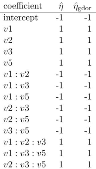
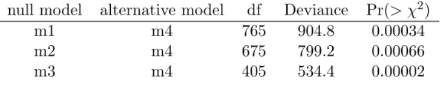
2.1 The estimated null eigenvector of inverse Fisher information matrix (column 2) and the gdor computed by Geyer (2009) (column 3). Only nonzero com-ponents are shown. . . 42 2.2 Model comparisons for Example 2. The model m1 is the main-effects only

model, m2 is the model with all two way interactions, m3 is the model with all three way interactions, and m4 is the model with all four way interactions. 44

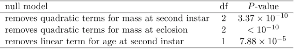
3.1 Rao tests for smaller models. P-values and degrees of freedom for Rao tests of three smaller models against the larger model that includes linear, quadratic, and interaction term for the two mass traits and a linear term for age at second larval instar stage. . . 60

4.1 Comparison of the MLE and the partial envelope estimator for components of interest in Example 1. We can see that the envelope estimator is providing useful variance reduction. . . 88 4.2 Comparison of the MLE and the partial envelope estimator for components

of interest in Example 2. We can see that the envelope estimator is providing useful variance reduction. . . 90

5.1 Comparison of ˆβwand ˆβu=2. The first row is the Euclidean difference between vec( ˆβw) and vec( ˆβu=2) from the original dataset. The second row is the

spectral norm of the estimated variance of the difference of all bootstrap realizations of ˆβ_w∗ and ˆβu=2 with bootstrap sample sizeB =n. . . 105

(12)

List of Tables x

5.2 The bootstrap distribution of ûaspincreases, where ûis selected bybicand n(û=j) is the number of times bic selected envelope dimensionj. . . 106 5.3 Averaged ratios of estimated standard errors across 25 replications of the

multivariate residual bootstrap at different numbers of resamples B for the fifth element of estimates ofβ. . . 107 5.4 Comparison of ˆβw and ˆβu=2, ˆβu=3, and ˆβu=4. The rows are the Euclidean

difference between vec( ˆβw) and the indicated envelope estimator from the

original dataset. . . 108

6.1 Comparison of bootstrapped standard errors to the true standard errors across three sample sizes in the fixed design case. The bootstrap sample size is set atB = 4nfor each dataset. . . 116 6.2 Comparison of bootstrapped standard errors to the true standard errors

across three sample sizes in the random design case with heteroskedastic-ity. The bootstrap sample size is set at B= 4nfor each dataset. . . 117

8.1 Simulation results. The first column displays the type of addition. The second column displays the data generating mechanism. The third column displays the additive parameter generating mechanism. The distributions in the third column have been scaled to have a mean of 0.5 and a standard deviation of 0.1. The random variables Y1 through Y3 are given below. The fourth column displays the p-values of the Kolmogorov–Smirnov test com-paring to the fixed parameter settingq=κ= 1/2. The final column displays the proportion of Shapiro–Wilks p-values exceeding 0.05. A Shapiro–Wilks p-value greater than 0.05 suggests that the asymptotic distribution of the random combination is log-normal (Tsallis case) or sinh-normal (Kaniadakis case) whereq=κ= 1/2. . . 175

(13)

List of Figures

2.1 All possible values of the canonical statistic MT_Y _{for the logistic regression}

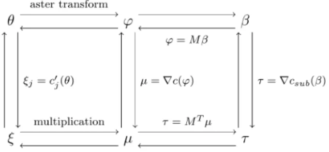
example in the Motivating Example section. The solid dot is the observed value ofMTY. . . 6 3.1 Graphical structure of the aster model for theE. angustifolia data. . . 48 3.2 A depiction of the transformations necessary to change parameterizations. . 51 3.3 Aster Graph for FemaleM. sexta. Arrows go from predecessor nodes to

suc-cessor nodes. Lines (that are not arrows) link dependence groups. Nodes are labeled by their associated variables. P node is pupation,T nodes are sur-vival and eclosion indicators,Bnodes are ovariole counts. Subscripts indicate age (in days), subsubscripts indicate variables in the same dependence group (0 = death, 1 = surviving but pre-eclosion, 2 = eclosion at this time). For simplicity, all deaths after pupation but before reproduction were modeled as occurring on day 33. No individuals survived past day 40. . . 57

(14)

List of Figures xii

3.4 Fitness landscapes without (left column) and with (right column) adjustment for population growth rate λ. Rows top to bottom are 2nd instar stage reached at age 2, 3, 4, and 5. Numbers on contours are absolute fitness (unconditional expected ovariole counts) in the left column and are relative fitness (absolute fitness divided by its average over the population) in the right column. All plots display fitness as contours vs. mass at eclosion and mass at 2nd instar stage. Boxes denote locations of maxima. The maximum values for unconditional expected ovariole counts for each age are 363.6 (age 2), 342.4 (age 3), 322.4 (age 4), and 303.6 (age 5). . . 61

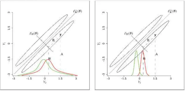
4.1 Visualization of the envelope model and the efficiency gains it is capable of producing.Graphic is taken from Su and Cook (2011). . . 73 4.2 (A) Graphical structure of the aster model for one individual in the E.

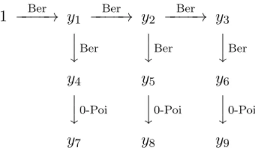
an-gustifoliadata. The top layer corresponds to survival; these random variables are Bernoulli. The middle layer corresponds to flowering; these random vari-ables are also Bernoulli. The bottom layer corresponds to flower head counts; these random variables are zero-truncated Poisson. (B) Graphical structure of the aster model for the data in Example 2. The first arrow corresponds to survival which is a Bernoulli random variable. The second arrow corresponds to reproduction count conditional on survival which is a zero-truncated Pois-son random variable. (C) Graphical structure of the aster model for the simulated data in Example 1. The top layer corresponds to survival; these random variables are Bernoulli. The middle layer corresponds to whether or not an individual reproduced; these random variables are also Bernoulli. The bottom layer corresponds to offspring count; these random variables are zero-truncated Poisson. . . 77 4.3 Algorithm 1. Parametric bootstrap envelope estimation of υ using the 1D

(15)

List of Figures xiii

4.4 Algorithm 2. Parametric bootstrap envelope estimation ofυ using reducing

subspaces. . . 86

4.5 Contour plots for the ratios of se (h(ˆτ)) to se (h(ˆτenv)) in Example 1. Ratios greater than 1 indicate efficiency gains using envelope methodology. . . 89

4.6 Contour plots for the ratios of se (h(ˆτ)) to se (h(ˆτenv)) in Example 2. Ratios greater than 1 indicate efficiency gains using envelope methodology. . . 91

7.1 Design space forπ1 andπ2in original units (a) and discretized and scaled to [−1,1]2 . . . 142

7.2 V-optimal designs for first- through fourth-order approximating polynomials forn= 16 . . . 144

7.3 The multivariate design: g₁ is a full third-order polynomial in π1 andπ2; g₁ is a quadratic inπ2 only. . . 145

7.4 V¯-optimal design given equal weighting of the first- through fourth-order approximating polynomials forn= 16 . . . 145

7.5 Combinations ofQ, n, and D that yieldπ1= 0.5×10−6 . . . 147

7.6 Trade-off (w-trace) plot for robust DA designs . . . 148

7.7 DA designs for the χ-space and forχπ-space for varying w . . . 149

8.1 Evidence for the existence of a universal limit law. The sampling distributions for the simulation settings in Table 8.1 are plotted here. The left panel displays the density curves corresponding to the Tsallis case. The right panel displays the density curves corresponding to the Kaniadakis case. The green lines correspond to density curves for the fixed q = κ = 1/2 case for both data generating distributions and both addition operations. . . 171

(16)

List of Figures xiv

8.2 The random variables are generated as X ∼ U(−2,2) for all sampling dis-tributions in both panels. The sampling disdis-tributions are constructed with twenty thousand samples of size n= 1000. The left panel depicts sampling distributions for Tsallis addition at three fixedq values and one random de-formation withq _∼ U(0,1). The right panel depicts sampling distributions for Kaniadakis addition at three fixedκvalues and one random deformation withκ∼U(0,1). . . 172

(17)

Chapter 1

Introduction

Statistical inference is the process of drawing conclusions about a population on the basis of measurements or observations made on a sample of units from the population (Everitt and Skrondal, 2010). The primary focus of this dissertation is the study of statistical inference when multiple variables are of interest. In particular, we focus on estimation of an unknown parameter vector of a data generating model and estimation of the estimator’s variability. The topics studied in this dissertation are varied but this is a main unifying theme. It is of specific interest to place realistic assumptions on the data generating model so that statistical inferences are reliable when made by practitioners in applications.

Outside of the common theme of multivariate statistical inference under realistic as-sumptions of the data generating model, the topics studied in this dissertation have little in common. The work in Chapters 2 through 4 put inferential interest in the canonical and mean-value parameter vectors of an exponential family. In Chapter 2, the exponential family is required to be discrete. In Chapters 3 and 4, the exponential family can be a mixture of discrete and continuous parts. The theory in Chapter 2 provides an inferential framework when observed data from a discrete exponential family is on the boundary of the support of the exponential family. Our theorems allow for practitioners to make relatively fast statistical inferences in this setting. Chapter 3 provides the backdrop of aster models, their usefulness in life history analysis, and contains a thorough real data example of them. The methods in Chapter 4 allow practitioners of life history analyses to estimate parameters of interest consistently and with less variability than existing methods can.

(18)

Chapter 1. Introduction 2

In Chapters 4 and 5, inferential interest is placed on consistent estimation and variance reduction through envelope methodology. In both chapters, model selection variability and post-selection inference are taken into account. The focus in these chapters is not to develop a framework for consistent model selection. Rather, models are averaged where the weight corresponding to a particular model reflects our belief that that particular model is the data generating model.

Bootstrapping techniques for inference in multivariate models are studied in Chapters 4 through 6. In Chapter 4, Efron (2014)’s parametric double bootstrap was used for inferences. In Chapter 5, a residual bootstrap of our construction was used for inferences. In Chapter 6, we extend the work of Freedman (1981) to show that the variability of the ordinary least squares regression coefficient matrix in the multivariate linear regression model is estimated consistently by the same residual bootstrap procedure as Freedman (1981).

In Chapter 7, we extend the work of Albrecht, Nachtsheim, Albrecht, and Cook (2013) to the multivariate design of experiments context. This provides a framework for practitioners to design efficient experiments when inference is desired for multiple responses that are measured in units that are otherwise not comparable. This work provides needed design of experiments methodology for a class of problems where appropriate and efficient designs were previously not well understood.

The work in Chapter 8 does not fit the multivariate theme or the same statistical inference theme as the work in the previous six chapters. However, it is work that I found interesting and completed during my tenure at the University of Minnesota. In this chapter, central limit theorems are developed when random variables are combined via a general binary operator instead of addition. Such central limit theorems are appropriate in physical applications.

All of the proofs in this dissertation are original to the author of this dissertation, except for the proof of Theorem 8. Theoretical derivations not made by this author are referenced.

(19)

Chapter 2

Maximum Likelihood Estimation

in Exponential Families

2.1 Introduction

We develop an inferential framework for discrete exponential family problems when observed data lies on the boundary of the support of the exponential family. In such settings, it may be the case that the maximum likelihood estimator (MLE) need not exist in the traditional sense but may exist in a completion of the exponential family. Completions for families with finite and countable support were considered by Barndorff-Nielsen (1978, 154-156) and Brown (1986, 191-201) respectively. Csisz´ar and Mat´uˇs (2005) generalized the notion of completion of exponential families and provided weak convergence results within their construction. Geyer (2009) developed an inferential framework for when MLEs exist in the completion of the exponential family. Geyer (2009) assumed the conditions mentioned in Brown (1986) and referred to the completion of the exponential family as the Barndorff-Nielsen completion of the exponential family. We will make the same reference. When it is the case that the MLE exists in the Barndorff-Nielsen completion of the exponential family, the traditional theory of MLEs and computational methods will lead their users astray (Geyer, 2009). Further complicating the issue is the fact that statistical software provides users with no reliable detection methods and solutions when the MLE exists in the Barndorff-Nielsen completion.

(20)

2.1. Introduction 4

Geyer (1990, 2009) provided a theoretical solution to this problem. Geyer (1990, Chap-ter 2) gave an algorithm that uses linear programming to calculate the MLE in a closed convex exponential family by recursively calculating limiting conditional models (LCMs) determined by directions of recession calculated by linear programming. A direction of recession is a direction that increases the likelihood of an exponential family as one goes further in that direction. An LCM is a model that is conditional on the subset of domain that is orthogonal to the direction of recession. Geyer (2009) gives an algorithm that uses linear programming to calculate the MLE in full regular exponential families satisfying a number of assumptions (Geyer, 2009, Section 3.7), by non-recursively calculating one LCM determined by a generic direction of recession calculated by linear programming. The al-gorithm in Geyer (1990, Chapter 2) is more general; the alal-gorithm in Geyer (2009) is more efficient for the special cases to which it applies. Neither is very fast, and neither scales to very large problems. According to the documentation for thecddlibcomputational geom-etry library, to which the R packagercdd provides an R interface, it can handle problems having number of variables in the low hundreds and number of constraints in the thou-sands. Put in the context of exponential family problems discussed by Geyer (2009) this corresponds to generalized linear models with a few hundred regression coefficients and less than ten thousand cases. But for problems even that large, the computational geometry calculations will be very slow. Computational geometry calculations using rcdd do have the virtue that they are exact, using infinite-precision rational arithmetic. They find exact directions of recession.

A much faster alternative is to just let maximum likelihood estimation find directions of recession. If we have a sequenceθn that maximizes the likelihood, we will have convergence

to the unique MLE distribution, provided it exists in the Barndorff-Nielsen completion. We justify this approach to maximum likelihood estimation by showing that cumulant generating functions (CGFs) evaluated at such a sequence of iterates converges to the CGF of the MLE distribution.

It is then shown that moments of all orders converge along the maximizing likelihood sequence θn. Inference about the canonical parameter vector of an exponential family

(21)

2.2. Motivating Example 5

can therefore be made when the MLE does not exist in the traditional sense. The CGF convergence that we develop is reliant on a measure-theoretic formulation of exponential families and on properties of sequences of affine functions. Both topics are thoroughly discussed before our convergence results are stated and examples are given.

Theorem 5 of Geyer (2009) in Section 2.4.5 and the following discussion state how taking limits in the generic direction of recession maximizes the likelihood. The LCM resulting from taking limits supports values of the canonical statistic that are orthogonal to the generic direction of recession. Therefore the direction of recession is a null eigenvector of the Fisher Information matrix of the LCM. Convergence of moments of all orders along maximizing likelihood sequences implies that we can estimate Fisher Information in the LCM without using directions of recession.

2.2 Motivating Example

Consider the case of perfect separation in the logistic regression model as an example of a discrete exponential family with data on the boundary of its support. In this example, suppose that we have a univariate response variabley and a single predictorxand suppose thatxj = 10j and yj = I{x>45}(xj) for j = 1, ...,8. Let β ∈R be the unknown regression

coefficient. The logistic regression model for this data has log likelihood given by

l(β) = 8 X j=1 yjlog eβxj 1 +eβxj + (1−yj) log 1 1 +eβxj = 8 X j=1 yj log eβxj 1 +eβxj −log 1 1 +eβxj + 8 X j=1 log 1 1 +eβxj =_hY, M β_{i −}c(β) =_hMTY, β_{i −}c(β) (2.1)

where Y is the vector of observed responses, M = (10, ...,80)T is the model matrix, and c(β) =−P8j=1log

1 1+eβxj

is the cumulant function of the exponential family. In the final parameterization of the model (2.1), we say that MT_Y _{is the canonical statistic and} _β _is

(22)

2.3. Laplace transforms and standard exponential families 6

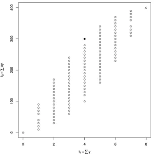
Figure 2.1: All possible values of the canonical statistic MTY for the logistic regression example in the Motivating Example section. The solid dot is the observed value ofMTY.

the canonical parameter of the exponential family. Because of perfect separation of the observed data, the MLE of β does not exist in the traditional sense. Consult Figure 2.1 to see that the canonical statistic exists on the boundary of its support in this example. Our theory provides an inferential context in this specific “perfect separation” in logistic regression setting as well as a more general setting where the MLE does not exist in the traditional sense.

2.3 Laplace transforms and standard exponential families

We motivate exponential families through their measure-theoretical formulation starting with the log Laplace transform of the generating measure for the family. In this context, the log Laplace transform is called the cumulant function of the exponential family. The reason for this level of generality is that the CGF convergence we develop requires that the log density of the exponential family be an affine function of the data.

(23)

Let λbe a nonzero positive Borel measure on a finite-dimensional vector space E (pos-itive means λ(B)_≥ 0 for all Borel setsB and nonzero means λ(B)₆= 0 for some Borel set B). The log Laplace transform ofλ is the function c:E∗ →R defined by

c(θ) = log

Z

ehx,θiλ(dx), θ ∈E∗ (2.2)

(Geyer, 1990, Section 2.1), where E∗ is the dual space ofE (Geyer, 1990, Appendix A.1),

h ·, · iis the canonical bilinear form placingEandE∗in duality (same appendix), and Ris the extended real number system (Geyer, 1990, Appendix A.6), which adds the values_−∞ and +_∞to the real numbers.

If one prefers, one can takeE=E∗=Rp for somep, and define

hx, θi=

p

X

i=1

xiθi, x∈Rp andθ ∈Rp,

(and Geyer, 2009, does this), but here, like everywhere else linear algebra is used, the coordinate-free view of vector spaces offers more generality, is cleaner, and is more elegant. Also, as we are about to see, ifEis the sample space of a standard exponential family, then a subset of E∗ is the canonical parameter space, and the distinction between E and E∗ helps remind us that we should not consider these two spaces to be the same space.

A log Laplace transform is a lower semicontinuous convex function that nowhere takes the value _−∞ (the value +_∞ is allowed and occurs where the integral in (2.2) does not exist) (Geyer, 1990, Theorem 2.1). Theeffective domain of an extended-real-valued convex function conE∗ is

domc=_{θ _∈E∗:c(θ)<+_{∞ }}. For every θ_∈domc, the functionfθ:E→R defined by

(24)

is a probability density with respect toλ. Densities (2.3) have log likelihood

l(θ) =_hx, θ_{i −}c(θ). (2.4) The set _F = _{fθ :θ ∈Θ}, where Θ is any nonempty subset of domc, is called astandard

exponential family of densities with respect to λ. This family is full if Θ = domc.

It is useful to have terminology relating the family _F to the measure λ. We say _F is the standard exponential family generated by λ having canonical parameter space Θ, and we sayλ is thegenerating measure of_F.

A general exponential family (Geyer, 1990, Chapter 1) is a family of probability dis-tributions having a sufficient statisticX taking values in a finite-dimensional vector space E that induces a family of distributions on E that have a standard exponential family of densities with respect to some generating measure. Reduction by sufficiency loses no statis-tical information, so the theory of standard exponential families tells us everything about general exponential families (Geyer, 1990, Section 1.2).

In the context of general exponential families X is called the canonical statistic and θ thecanonical parameter (the terms natural statistic andnatural parameter are also used). In the context of standard exponential families, we only use the canonical parameter and statistic. The set Θ is the canonical parameter space of the family, the set domc is the canonical parameter space of the full family having the same generating measure. A full exponential family is said to be regular if its canonical parameter space domc is an open subset ofE∗.

The distributions Fθ corresponding to the densities (2.3) are given by

Fθ(B) =

Z

B

ehx,θi−c(θ)λ(dx), B _{∈ B}, (2.5)

(25)

2.4. Generalized affine functions 9

distribution has a CGF, is given by

kθ(t) = log

Z

ehx,tifθ(x)λ(dx)

=c(θ+t)₋c(θ)

(2.6)

and this is a CGF provided it is finite on a neighborhood of zero, that is ifθ _∈int(domc). We see that every distribution in a full family has a CGF if and only if the family is regular. Derivatives ofkθevaluated at zero are the cumulants of Fθ. These are the same as

derivatives of cevaluated at θ.

2.4 Generalized affine functions

2.4.1 Characterization on affine spaces

Exponential families defined on affine spaces are of particular interest for the convergence we develop. In the previous section, we motivated the development of the exponential family through its generating measure λ. The log likelihood of the exponential family corresponding to this measure-theoretic formulation is an affine function of the data as seen in (2.4). What we will call theBarndorff-Nielsen completion of the exponential family, following Geyer (2009), is the set of all limits of distributions in the family. We take limits in the sense of pointwise convergence of densities, following Geyer (1990, Chapters 2 and 4) and Geyer (2009). Other authors, including Barndorff-Nielsen (1978) and Brown (1986), have taken limits in the sense of convergence in distribution, but discussed no examples where convergence in distribution gave different results from pointwise convergence of densities.

Of course, ifehn _→_eh _{pointwise, then}_h

n→hpointwise, and vice versa. Hence the idea

of completing an exponential family naturally leads to the the study of limits of sequences of affine functions. Here we assume that the limiting function may be extended-real-valued (the extended real number system, denotedR, is the two-point compactification of the real number system, which adds −∞ at one end and +∞at the other). A real-valued function is affine if and only if it is both convex and concave. Since limits preserve convexity and

(26)

concavity, we are led to the study of extended-real-valued functions that are both convex and concave. These functions are calledgeneralized affine functions.

Geyer (1990, Chapter 3) studies generalized affine functions on both finite-dimensional and infinite-dimensional affine spaces, but here we only study generalized affine functions on finite-dimensional affine spaces. That is all that is needed for exponential family theory.

Definition 1

An extended-real-valued function h on a finite-dimensional affine space E is generalized

affine if it is both convex and concave.

This means that (Rockafellar, 1970, Section 4; Rockafellar and Wets, 1998, Section 2.A)

h x+t(y−x)≤(1−t)h(x) +th(y),

whenever 0< t <1 andh(x)<∞andh(y)<∞, and

h x+t(y₋x)_≥(1₋t)h(x) +th(y),

whenever 0< t <1 andh(x)>_−∞ andh(y)>_−∞. The former says h is convex. The latter says h is concave. The following two theorems provide a characterization of generalized affine functions on affine spaces. In preparation, we use the notation

h−1(R) =_{x_∈E:h(x)_∈R}

h−1(_∞) =_{x_∈E:h(x) =_{∞ }} h−1(_−∞) =_{x_∈E:h(x) =_{−∞ }}

Theorem 1

(27)

affine if and only if one of the following cases holds

(a) h−1₍_∞_{) =}_E, (b) h−1₍_−∞_{) =}_E,

(c) h−1(R) =E andhis an affine function,

(d) There is a hyperplane H such thath(x) =∞for all points on one side ofH, h(x) =

−∞for all points on the other side of H, andhrestricted toH is a generalized affine

function.

The proof of Theorem 1 is in Geyer (1990). The intention is that this theorem is applied recursively. If we are in case (d), then the restriction ofhtoH is another generalized affine function to which the theorem applies. More on this later.

2.4.2 Topology

Now we need to understand the topology of the space of generalized affine functions on a finite-dimensional affine spaceE with the topology of pointwise convergence. Call that G(E).

Theorem 2

The space of generalized affine functions on a finite-dimensional affine space with the topol-ogy of pointwise convergence is a compact Hausdorff space.

The proof of Theorem 2 is in Geyer (1990).

Theorem 3

G(E) is a first countable topological space.

The proof of Theorem 3 is in Geyer (1990). The spaceG(E) is not metrizable, unlessE is zero-dimensional (Geyer, 1990, penultimate paragraph of Section 3.3). So we cannot use δ-ε arguments, but we can use arguments involving sequences, in particular, a compact and

(28)

first countable topological space is sequentially compact (every sequence has a convergent subsequence) (Kelley, 1955, Chapter 5, Problem E, Part (d)). This is instrumental for our treatment of maximum likelihood estimation.

2.4.3 Characterization on vector spaces

The convergence results that we discover are aimed for application in generalized linear regression model problems with data that is assumed to be realized from a full discrete exponential family. In these applications, data and parameters are assumed to be elements of a finite-dimensional vector space. The conclusions of Theorem 3 hold whenG(E) is the space of generalized affine functions on a finite-dimensional vector spaceEwith the topology of pointwise convergence. The next Theorem provides a characterization of generalized affine functions defined on finite-dimensional vector spaces.

Theorem 4

An extended-real-valued function h on a finite-dimensional vector space E is generalized affine if and only if there exist finite sequences (perhaps of length zero) of vectors η1, . . . , ηj being a linearly independent subset ofE∗, the dual space of E, and scalars δ1, . . . , δj

such thathhas the following form. DefineH0=Eand, inductively, for integersisuch that 0< i≤j

Hi ={x∈Hi−1:hx, ηii=δi}

C_i+=_{x_∈Hi−1:hx, ηii> δi}

C_i−=_{x_∈Hi−1:hx, ηii< δi}

all of these sets (if any) being nonempty. Then h(x) = +∞ whenever x ∈C_i+ for any i, h(x) =_−∞wheneverx_∈C_i−for anyi, andhis either affine or constant onHj, where +∞

and_−∞ are allowed for constant values.

Proof: First, assumehsatisfies the conditions of Theorem 1 onE. We then show thath

(29)

hypothesis, H(p), is that the conclusions of Theorem 1 imply that the conclusions of The-orem 4 hold when dim(E) =p. We now show that H(0) holds. In this setting, E = _{0_}. Thus Theorem 4 holds withj= 0 andhis constant onE. The basis of the induction holds. Let dim(E) = p+ 1. We now show that H(p) implies that H(p+ 1) holds. In the event that h is characterized by case (a) or (b) of Theorem 1 then Theorem 4 holds with j= 0. If case (c) of Theorem 1 characterizeshthen there is an affine functionf1 defined by f1(x) =hx, η1i −δ1, x∈E, such thath(x) = +∞forxsuch thatf1(x)>0,h(x) =−∞for x such that f1(x)<0, and h is generalized affine on the hyperplane H1 ={x:f1(x) = 0}. The hyperplane H1isp-dimensional affine subspace ofE. Now, for some arbitraryζ1∈H1, define

V1={x−ζ1:x∈H1}

=_{y_∈E :_hy, η1i=δ1− hζ1, η1i} =_{y_∈E :_hy, η1i= 0}

where the last equality follows from ζ1 ∈ H1. The space V1 is a p-dimensional vector subspace ofEsince every affine space containing the origin is a vector subspace (Rockafellar, 1970, Theorem 1.1) and because every translate of an affine space is another affine space (Rockafellar, 1970, pp. 4). Let

h1(y) =h(y+ζ1), y∈V1. (2.7)

The functionh1is convex since the composition of a convex function with an affine function is convex. To see this, let 0< λ <1, picky1, y2∈V1 and observe that

h1(λy1+ (1−λ)y2) =h(λy1+ (1−λ)y2+ζ1)

≤λh(y1+ζ1) + (1−λ)h(y2+ζ1) =λh1(y1) + (1−λ)h1(y2).

(30)

A similar argument shows thath1 is concave. Therefore h1 is generalized affine. From our induction hypothesis, the conclusions of Theorem 1 imply that the conclusions of Theorem 4 hold for the generalized affine function h1. These conditions are that there exist finite sequences of vectors ˜η2, . . ., ˜ηj being a linearly independent subset of V1∗, the dual space of V1, and scalars ˜δ2, . . ., ˜δj such that h1 has the following form. Define He1 = V1 and, inductively, for integers isuch that 2< i_≤j

e Hi={x∈Hei−1:hx,η˜ii= ˜δi} e C_i+=_{x_∈Hei−1:hx,η˜ii>δ˜i} e C_i−=_{x_∈Hei−1:hx,η˜ii<δ˜i} (2.8)

all of these sets (if any) being nonempty. Thenh1(x) = +∞ whenever x∈Cei+ for any i,

h1(x) =−∞ wheneverx∈Ce_i− for anyi, and h1 is either affine or constant on Hej, where

+_∞and_−∞ are allowed for constant values.

It remains to show that the conditions of Theorem 4 hold with respect toh. The vectors ˜

ηi, i= 2, ..., j can be extended to form a set of vectors ηi, i = 2, ..., j in E∗ by the

Hahn-Banach Theorem (Rudin, 1973, Theorem 3.6). The vectorsηi, i = 2, ..., j, form a linearly

independent subset ofE∗. To see this, letPj_k₌₂akηk = 0 on E for scalars ak, k = 2, ..., j.

Then Pj_k₌₂akηk = 0 on V1 which implies that ak = 0 for k = 2, ..., j by the definition of

linearly independent. LetH0=E, and, for i= 2, ..., j, define

Hi={x∈Hi−1:hx, ηii=δi}

C_i+=_{x_∈Hi−1:hx, ηii> δi}

C_i−=_{x_∈Hi−1:hx, ηii< δi}

(2.9)

whereδi = ˜δi− hζ1, ηii for i = 2, ..., j andHei = Hi+ζ1 as a result. We see that h(x) = h1(x−ζ1) = +∞wheneverhx+ζ1, ηii>δ˜i. Thereforeh(x) = +∞for allx∈C_i+for anyi.

The same derivation shows thath(x) =_−∞ wheneverx_∈C_i− for anyi. The generalized affine function h is either affine or constant on Hj, where +∞ and −∞ are allowed for

(31)

We now show that the vectorsη1, ..., ηjare linearly independent. Assume thatPj_k₌₁akηk =

0 onE for scalarsak,k= 1, ..., j. This assumption implies thatP_kj₌₁akη˜= 0 onV1∗where ˜

η1 is the restriction of η1 to V1. Thus ˜η1 is an element of V1∗ and ˜η1 = 0 on V1 since

hy,η1˜ i = hy, η1i = 0 on V1. Therefore P_kj₌₂akη˜k = 0 where ak = 0 for k = 2, ..., j from

what has already been shown. In the event that a1 = 0, we can conclude that η1, ..., ηj

are linearly independent. Now consider a1 6= 0. In this case, Pjk=1akηk = 0 implies that

η1 = Pj_k₌₂bkηk where bk = −ak/a1. This states that Pj_k₌₂bkη˜k = 0 on V1. Therefore,

bk = 0 for allk = 2, ..., j which implies thatη1 is the zero vector, which is a contradiction. Thusa1 = 0 and we can conclude that η1, ..., ηj are linearly independent. This completes

one direction of the proof.

Now assume that h satisfies the conclusions of Theorem 4 and show that these con-clusions imply that Theorem 1 holds by induction on j. The induction hypothesis, H(j), is that the conclusions of Theorem 4 imply that the conclusions of Theorem 1 hold for sequences of lengthj. For the basis of the induction let j = 0. We now show that H(0) holds. The generalized affine functionh is either affine or constant on E where +∞ and

−∞are allowed for constant values. This characterization of h is the same as cases (a) of (b) of Theorem 1. The basis of the induction holds.

We now show that H(j) implies that H(j+ 1) holds. When the length of sequences is j+ 1, there exist vectors η1, ..., ηj+1 and scalars δ1, ..., δj+1 such that h has the following form. Define H0 = E and, inductively, for integers i, 0 < i ≤ j+ 1, such that the sets in (2.9) are all nonempty. Then h(x) = +_∞ whenever x _∈ C_i+ for any i, h(x) = _−∞ wheneverx_∈C_i−for anyi, andhis either affine or constant onHj+1, where +∞and−∞ are allowed for constant values. From the definition of the setsH1,C₁+, andC₁−, there is an affine functionf1defined byf1(x) =hx, η1i −δ1, x∈E, such thath(x) = +∞for allx∈E such that f1(x)>0 and h(x) =−∞ for all x∈E such that f1(x)< 0. This is equivalent to the case (c) characterization of hin Theorem 1, provided we show that the restriction of h toH1 is a generalized affine function.

Define V1 = H1−ζ1 for some arbitrary ζ1 ∈ H1. Let dim(E) = p. The space V1 is a (p−1)-dimensional vector subspace of E. Defineh1 as in (2.7). Let ˜ηi be the restriction

(32)

of ηi to V1 so that ˜ηi is an element of V1∗ for 1 < i ≤ j+ 1. Now let H1e = V1 and, for 1 < i _≤ j+ 1, we can define the sets as in (2.8) where ˜δi = δi− hζ1,η˜ii. We see that

h1(x) =h(x+ζ1) = +∞wheneverhx+ζ1, ηii>δ˜i. Therefore h1(x) = +∞for all x∈Cei+

for any i. The same derivation shows that h1(x) =−∞ wheneverx∈Ce_i− for anyi. The generalized affine function h1 is either affine or constant onHj+1, where +∞and −∞are allowed for constant values. Thereforeh1meets the conditions of Theorem 4 with sequences of length j. From H(j), we know that the conclusions of Theorem 1 hold with respect to

h1. This completes the proof.

2.4.4 Affine functions and exponential families

A family of probability distributions having densities with respect to a positive Borel mea-sure λ on a finite-dimensional affine (vector) space is a standard generalized exponential family if the densities of these distributions with respect toλ have the formeg _where_g_{is a}

generalized affine function. This definition is the same as Section 2 except for the replace-ment of exponential family by generalized exponential family and the replacement ofaffine function bygeneralized affine function.

Let x∈E be observed data realized from a closed convex standard exponential family with log likelihood (2.4). Let the parameter space Θ_⊆E∗ and definem(x) = sup_θ_∈_Θl(θ). Then, for any xsuch that m(x)<_∞, there is a sequence θn ∈Θ such that

l(θn)→m(x), as n→ ∞. (2.10)

From sequential compactness of G(E), which arises as a consequence of Theorem 3, there is a subsequence θnk such that the sequence of affine functions defined by

hθ_nk(x) =hx, θnki −c(θnk), y∈E,

converges pointwise to a generalized affine function h_∈G(E). Since hθ_nk(x) =hx, θnki −c(θnk) =l(θnk)→m(x),

(33)

we haveh(x) =m(x) whereehis a density corresponding to a generalized exponential family. This treatment of maximum likelihood estimation is different from the usual situation in which we find the parameter value which maximizes the likelihood. Instead, a sequence of log densities, interpreted as affine functions, converges to the maximum likelihood estimator m(x). In this case, the MLE is a generalized affine functionh_∈G(E).

If we take a pointwise limit of a sequence of densities ehi _{in the family, the limit will} have the form eg, where g is a generalized affine function. From Fatou’s lemma, we know that Reg_dλ _≤ _{1. Thus we say such limits are} _{subprobability densities. In general, one}

does get subprobability densities that are not probability densities as limits of sequences in exponential families (Geyer, 1990, Examples 4.1, 4.2, 4.3, 4.4, and 4.5). But one does not get subprobability densities that are not probability densities as limits of sequences in discrete closed convex exponential families, including discrete full exponential families (Geyer, 1990, Theorem 2.7).

To establish CGF convergence in the next section, we represent the likelihood maxi-mizing sequence in the coordinates of the linearly independentη vectors that characterize the generalized affine functionh according to its Theorem 4 representation. Leth be rep-resented as in Theorem 4 with j _≤ p. From Theorem 4, we have a linearly independent set of vectors η1, ..., ηj ∈ E∗. We can extend this linearly independent set of vectors to

form a basis for E∗ by finding vectors ηj+1, ..., ηp (Friedberg, et al., 2003, Corollary 2 to

Theorem 1.10). Since η1, ..., ηp is a basis for E∗, we can express the sequence of iterates

which maximizes the likelihood as

θn=b1,nη1+b2,nη2+· · ·+bp,nηp. (2.11)

Define ψn = Pp_i₌_j₊₁bi,nηi and let ci denote the log Laplace transform of the measure λ

restricted to the hyperplane Hi for i = 1, ..., j. Lemma 1 provides properties about the

numbersbi,n, i= 1, ..., pneeded to prove CGF convergence.

Lemma 1

(34)

at at least one point. Representhas in Theorem 4, and extend η1, . . . , ηj to be a basisη1,

. . . , ηp forE∗. Then there are sequences of scalarsan andbi,n such that

hn(y) =an+ j X i=1 bi,n(hy, ηii −δi) + p X i=j+1 bi,nhy, ηii, y∈E, (2.12)

where the rightmost sum in (2.12) is empty whenj=pand, asn→ ∞, we have (a) bi,n→ ∞, for 1≤i≤j,

(b) bi,n/bi−1,n→0, for 2≤i≤j+ 1,

(c) bi,n converges, fori > j, and

(d) an converges

if and only if hn converges to honE.

Proof: First suppose that hn converges toh. The assumption thath is finite at at least

one point guarantees that h is affine onHj from Theorem 4. For all y∈Hj we can write

h(y) =_hy, θ∗i+a where_hy, θ∗i=Pp_i₌_j₊₁dihy, ηiiands, di ∈R. The convergence hn →h

implies that bi,n →di, i= j+ 1, ..., p where the set of bi,ns is empty whenj =p and that

an →aasn→ ∞. Thus conclusions (c) and (d) hold. To show that conclusions (a) and (b)

hold we will suppose that j >0, because these conclusions are vacuous when j= 0. Both cases (a) and (b) will be shown by induction with the hypothesis H(m) thatb(j−m),n→+∞

and b(j−m+1),n/b(j−m),n →0 asn→ ∞for 0≤m≤j−1. We now show that the basis of

this induction holds. Pick y_∈C_j+ and observe that

hn(y) =an+bj,n(hy, ηji −δj) + p

X

k=j+1

bk,nhy, ηki →+∞.

since h(y) = +∞ and hn → h pointwise. From this, we see that bj,n → +∞ as n→ ∞

and bj+1,n/bj,n → 0 as n → ∞ from part (c). Therefore H(0) holds. It is now shown

(35)

space of E∗, such that hyi, ηki = 0 when i =6 k and hyi, ηki = 1 when i = k. The set of

vectorsy1, ..., yp is a basis ofE sinceE=E∗∗. Arbitrarily choose ay∈Hj−m−1 such that y = Pj_i₌₁−m−1δiyi+c1yj−m where c1 > δj−m. At this choice of y we see that h(y) = +∞

and hn(y) =an+ j−_Xm+1 i=1 bi,n(hy, ηii −δi) =an+b(j−m),n(hy, ηj−mi −δj−m) →+_∞

asn_{→ ∞}. Thereforeb(j−m),n→+∞asn→ ∞. Now arbitrarily choosey=Pji=1−m−1δiyi+

c1yj−m+c2yj−m+1 where c1 is defined as before and c2 < δj−m+1. At this choice ofy we

see that h(y) = +_∞and hn(y) =an+ j−_Xm+1 i=1 bi,n(hy, ηii −δi) =an+b(j−m),n(hy, ηj−mi −δj−m +b(j−m+1),n b(j−m),n (_hy, ηj−m+1i −δj−m+1) =an+b(j−m),n c1−δj−m− b(j−m+1),n b₍_j₋_m₎_,n (c2−δj−m+1) →+∞ (2.13)

asn_{→ ∞}. It follows from (2.13) that

c1−δj−m− b₍_j₋_m₊₁₎_,n b(j−m),n (c2−δj−m+1) ≥0 for sufficiently largen. This implies that

b(j−m+1),n

b(j−m),n ≤

c1−δj−m

(36)

for sufficiently large n. From the arbitrariness of the constants c1 and c2 and (2.13), we can conclude that b₍_j₋_m₊₁₎_,n/b₍_j₋_m₎_,n _→0 as n_{→ ∞}. Therefore H(m+ 1) holds and this completes one direction of the proof.

We now assume that conditions (a) through (d) and the hn takes the form in (2.12).

Let limn→∞Ppi=j+1bi,nηi =θ∗ and limn→∞an=a. Cases (a) through (d) then imply that

hn(y)→          −∞, y_∈C_i− hy, θ∗i+a, y_∈Hj +∞, y∈C_i+ (2.14)

for alli = 1, ..., j where the right hand side of (2.14) is a generalized affine function in its

Theorem 4 representation. This completes the proof.

The results given in Lemma 1 are applicable to generalized affine functions in full gener-ality. However, specifics of interest arise whenehis a density corresponding to a generalized exponential family andhn =hθncorresponds to a likelihood maximizing sequence satisfying (2.10). Suppose that there arejhyperplanes characterizinghas in Theorem 4 and letθ∗be the maximum likelihood estimator corresponding to the model restricted to the hyperplane Hj. We now provide a brief extension of Lemma 1 that is consistent with this setup.

Corollary 1

For data x from a regular full exponential family defined on a vector space E, suppose θn is a likelihood maximizing sequence satisfying (2.10) with log densities hn converging

pointwise to a generalized affine functionh. Characterize has in Theorem 4 and represent the sequence θn in coordinate form as in (2.11). Define ψn = Pp_i₌_j₊₁bi,nhx, ηii. Then

conclusions (a) and (b) of Lemma 1 hold in this setting and

ψn→θ∗, asn→ ∞,

whereθ∗ is the MLE of the exponential family restricted to Hj.

(37)

Lemma 1 are satisfied. As a consequence,ψn →θ∗asn→ ∞. The fact thatθ∗is the MLE

of the LCM restricted toHj follows from our assumption thatθn is a likelihood maximizing

sequence.

Taken together, Theorem 4, Lemma 1, and Corollary 1 provide a theory of maximum likelihood estimation in exponential families motivated by properties of sequences of affine functions on finite-dimensional vector spaces. One key difference of this theory and the traditional theory is that the MLE is not a parameter value,θ∈Θ, but rather a log density h _∈ G(E). These different formulations are the same when the data from a regular full exponential family are in the interior of their support set. In this case, we can write

h(x) =_hx,θˆ_{i −}c(ˆθ)

where ˆθ _∈Θ is the MLE that satisfiesh(x) =m(x) and the generalized affine functionh is affine. When we represent h as in Theorem 4 in this case, we have that j = 0. However, when the observed data are on the boundary of their support, the MLE does not exist in the traditional sense and may exist in the Barndorff-Nielsen completion. Our theory can find the MLE in the Barndorff-Nielsen completion of the exponential family in this setting whenm(x)<_∞.

2.4.5 Comparisons with Geyer (2009)

We are not the only ones to investigate the existence of the MLE in the Barndorff-Nielsen completion of an exponential family when data are on the boundary of their support. Geyer (2009) investigated this issue and found the MLE in what is called a limiting conditional model (LCM). In practical settings, the support set for an LCM is determined by an es-timated generic direction of recession (GDOR). The GDOR and LCM approach to this problem is similar to our approach, as evidenced by Theorem 5. Let K denote the convex support of the measure λ. The convex support of λis the smallest closed convex set whose complement hasλmeasure zero (Barndorff-Nielsen, 1978, p. 90).

(38)

2.4. Generalized affine functions 22 Theorem 5

For a full exponential family having log likelihood (2.4), densities (2.3), natural statisticX, observed value of the natural statisticx such thatx_∈K, and natural parameter space Θ, ifη is a direction of recession,

Hη ={w∈Rp:hw−x, ηi= 0},

and pr(X _∈Hη)>0 for some distribution in the family, and hence for all, then for allθ∈Θ

lim s→∞fθ+sη=              0, hX(w)−x, ηi<0 fθ(w)/prθ(X ∈Hη), hX(w)−x, ηi= 0 +_∞, _hX(w)₋x, η_i>0 (2.15)

Ifη is not a direction of constancy, then s _7→ pr_θ₊_sη(X _∈Hη) is continuous and strictly

increasing, and pr_θ₊_sη(X ∈Hη)→1 ass→ ∞.

Proof: A proof is given in Geyer (2009).

As stated in Geyer (2009, Section 3.4) there are three things to note about the right-hand side of (2.15). First, it is a probability density function with respect to the distribution having parameter value ψ. From Geyer (2009, Theorem 3 (d)), the set where it is +∞

has probability zero. Second, it is the density with parameter value θ of the conditional distribution given that X ∈ Hη. Third, by Scheffe’s lemma (Lehmann, 1959, pp. 351)

pointwise convergence of densities implies convergence in total variation, which implies convergence in distribution. Denote the right-hand side of ((2.15)) byfθ(w|X ∈Hη). It is

clear that the family

{fθ(·|X ∈Hη) :θ∈Θ} (2.16)

is an exponential family with the same natural statistic and natural parameter as the original family. It need not be full. The natural parameter space of the full family containing it is

(39)

at least as large as

Θ + Γlim={θ+γ :θ∈Θ and γ∈Γlim}, (2.17)

whereθ is the natural parameter space of the original family and Γlimis the constancy space of the family (2.16). We will assume that (2.17) is the natural parameter space of the full family containing (2.16), and we will call this full family the LCM. It is clear that the log likelihood for (2.16)

lHη(θ) =hx, θi −c(θ)−log prθ(X ∈Hη)

satisfies

l(θ)< lHη(θ), θ ∈Θ.

Thus, if an MLE exists for the LCM, then it maximizes the likelihood in the family that is the union of the LCM and the original family, and it maximizes the likelihood in the family that is the set of all limits of sequences of distributions in the original family. When this happens, we say we have found an MLE in the Barndorff-Nielsen completion of the original family.

Refer back to the perfect separation case in logistic regression mentioned in Section 2.2. The GDOR for this examples is ˆηgdor= (−5,0.1)T and the LCM is degenerate at the observed data. The set Hη is the one point set containing only the observed value of the

canonical statistic.

In Geyer (2009), the solution to finding an MLE in the Barndorff-Nielsen completion of the original family is dependent upon estimation of a direction of recession and then taking limits in that direction, as seen in Theorem 5. In our approach, we allow the iterates of a likelihood maximizing sequence (2.10) to find the MLE in the LCM. We compare methods from a practical standpoint in Section 5. In the next section, we provide convergence results necessary for inference when maximum likelihood estimation is obtained through an arbitrary likelihood maximizing sequence (2.10).

(40)

2.5. Convergence theorems 24

2.5 Convergence theorems

We now show CGF convergence along a likelihood maximizing sequence (2.10). First define cA(θ) = logR_Aehy,θiλ(dy) for all θ ∈domcA = {θ : cA(θ) < +∞}. Define the CGF with

respect to the generalized affine function hby

κ(t) = log

Z

ehy,tieh(y)λ(dy)

for all t ∈ Rp such that κ(t) is finite. Define the CGF along the likelihood maximizing sequence (2.10) with respect to the log densitieshn by

κn(t) = log

Z

ehy,tiehn(y)λ(dy)

for allt_∈Rp such that κ(t) is finite where hn converges to a generalized affine function h.

In the next theorem, we state the conditions for whichκn(t)→κ(t).

Theorem 6

Let E be a finite-dimensional vector space of dimension p. For data x ∈E from a regu-lar full exponential family with natural parameter space Θ ⊆ E∗ and generating measure λ. Assume that all LCMs are regular exponential families. Suppose that θn is a

likeli-hood maximizing sequence satisfying (2.10) with log densities hn converging pointwise to

a generalized affine function h. Characterize h as in Theorem 4. When j _≥ 2, and for i= 1, ..., j₋1, define

Di={y∈Ci−:hy, ηki> δk, somek > i},

F =E_{\ ∪}j_i₌₁−1Di={y:hy, ηii ≤δi, 1≤i≤j},

(2.18)

and assume that

sup θ∈Θ sup y∈∪ji=1−1Di ehy,θi−c∪j−1 i=1Di (θ) <_∞ or λ_∪j_i₌₁−1Di = 0. (2.19)

(41)

Thenκn(t) converges to κ(t) pointwise for alltin a neighborhood of 0.

Proof: First consider the case when j = 0, the sequences of η vectors and scalars δ

are both of length zero. There are no sets C+ _and _C− _{in this setting and} _h _{is affine}

on E. From Lemma 1 we have ψn = θn. From Corollary 1, θn → θ∗ as n → ∞. We

observe that c(θn) → c(θ∗) from continuity of the cumulant function. The existence of

the MLE in this setting implies that there is a neighborhood about 0 denoted by W such that θ∗+W _⊂int(domc). Pick t_∈W and observe that c(θn+t)→c(θ∗+t). Therefore

κn(t)→κ(t) whenj= 0.

Now consider the case when j = 1. Define c1(θ) = logR_H₁ehy,θiλ(dy) for all θ ∈ int(dom c1). In this scenario we have

κn(t) =c(ψn+t+b1,nη1)−c(ψn+b1,nη1)

=c(ψn+t+b1,nηj)−c(ψn+b1,nη1)±b1,nδ1

= [c(ψn+t+b1,nη1)−b1,nδ1]−[c(ψn+b1,nη1)−b1,nδ1].

From Geyer (1990, Theorem 2.2), we know that

c θ∗+t+sη1−sδ1 →c1 θ∗+t, c θ∗+sη1−sδ1 →c1 θ∗,

(2.20)

as s_{→ ∞} sinceδ1 ≥ hy, η1i for ally ∈H1. The left hand side of (2.20) is a convex func-tion of θ and the right hand side is a proper convex function. If int(domc1) is nonempty, which holds whenever int(dom c) is nonempty, then the convergence in (2.20) is uniform on compact subsets of int(dom c1) (Rockafellar and Wets, 1998, Theorem 7.17). Also (Rock-afellar and Wets, 1998, Theorem 7.14), uniform convergence on compact sets is the same as continuous convergence. Using continuous convergence, we have that both

c(ψn+t+b1,nη1)−b1,nδ1→c1 θ∗+t, c(ψn+b1,nη1)−b1,nδ1→c1 θ∗,

(42)

whereb1,n→ ∞as n→ ∞by Lemma 1. Thus

κn(t) =c(θn+t)−c(θn)→c1 θ∗+t−c1 θ∗ = log

Z

H1

ehy+t,θ∗i−c(θ∗)λ(dy) = log

Z H1 ehy,ti+h(y)λ(dy) = log Z ehy,ti+h(y)λ(dy) =κ(t).

This concludes the proof whenj= 1.

For the rest of the proof we will assume that 1< j _≤pwhere dim(E) =p. Represent the sequenceθn in coordinate form as in (2.11) with scalars bi,n,i= 1, ..., p. For 0< j < p, we

know thatψn →θ∗ asn→ ∞ from Corollary 1. The existence of the MLE in this setting

implies that there is a neighborhood about 0, denoted byW, such thatθ∗+W _⊂int(domc). Pickt_∈W, fixε >0, and constructε-boxes aboutθ∗andθ∗+t, denoted by_N0,ε(θ∗) and

Nt,ε(θ∗) respectively, such that bothN0,ε(θ∗),Nt,ε(θ∗)⊂int (domc). LetVt,εbe the set of

vertices of_Nt,ε(θ∗). For all y∈E define

Mt,ε(y) = max v∈Vt,ε{h

v, yi}, Mft,ε(y) = min v∈Vt,ε{h

v, yi}. (2.21)

From the conclusions of Lemma 1 and Corollary 1, we can pick an integer N such that

hy, ψn+ti ≤Mt,ε(y) and b(i+1),n/bi,n <1 for alln > N andi = 1, ..., j−1. For all y∈F,

we have hy, θn+ti − j X i=1 bi,nδi =hy, ψn+ti+ j X i=1 bi,n(hy, ηii −δi) ≤Mt,ε(y) (2.22)

for alln > N. The integrability ofeMt,ε(y) _and_eMft,ε(y) _{follows from}

Z eMft,ε(y)λ(dy)≤ Z eMt,ε(y)λ(dy) = X v∈Vt,ε Z {y:hy,vi=Mt,ε(y)} ehy,viλ(dy)

(43)

2.5. Convergence theorems 27 ≤ X v∈Vt,ε Z ehy,viλ(dy)<_∞. Therefore, hy, ψn+ti+ j X i=1 bi,n(hy, ηii −δi)→    hy, θ∗+t_i, y_∈Hj, −∞, y∈F \Hj.

which implies that

cF(θn+t)−cF(θn)→cHj(θ∗+t)−cHj(θ∗) (2.23)

by dominated convergence. To complete the proof, we need to verify that

c(θn+t)−c(θn) =cF(θn+t)−cF(θn) +c_∪j−1 i=1Di(θn+t)−c∪j −1 i=1Di(θn) →cHj(θ∗+t)−cHj(θ∗). (2.24)

We know that (2.24) holds whenλ(∪ji=1−1Di) = 0 in (2.19) because of (2.23). Now suppose thatλ(_∪j_i₌₁−1Di)>0. We have, hy, ψn+ti+ j X i=1 bi,n(hy, ηii −δi)→ −∞, y∈ ∪j_i₌₁−1Di, (2.25)

(44)

2.5. Convergence theorems 28 and expc_∪j−₁ i=1Di(θn+t)−c∪j −₁ i=1Di(θn) = Z ∪j_i₌₁−1Di ehy,θn+ti−c∪j−1 i=1Di (θn) λ(dy) ≤ Z ∪ji=1−1Di eMt,ε(y)−Mf0,ε(y)+hy,θni−c∪j−1 i=1Di (θn) λ(dy) ≤ sup y∈∪ji=1−1Di ehy,θni−c∪j−1 i=1Di (θn) λ_∪j_i₌₁−1Di × Z ∪ji=1−1Di eMt,ε(y)−Mf0,ε(y)_λ(dy) ≤sup θ∈Θ sup y∈∪ji=1−1Di ehy,θi−c∪j−1 i=1Di (θ) λ∪ji=1−1Di × Z ∪j_i₌₁−1Di eMt,ε(y)−Mf0,ε(y)_λ(dy) _< _∞ (2.26)

for all n > N by the assumption given by (2.19). The assumption that the exponential family is discrete and full implies that Reh(y)λ(dy) = 1 (Geyer, 1990, Theorem 2.7). This in turn implies that λ(C_i+) = 0 for all i = 1, ..., j which then implies that c(θ) = cF(θ) +

c_∪j−₁

i=1Di(θ).Putting (2.22), (2.25), and (2.26) together we can conclude that (2.24) holds as n_{→ ∞} by dominated convergence and

cHj(θ∗+t)−cHj(θ∗) = log

Z

Hj

ehy,θ∗+tiλ(dy)−log

Z Hj ehy,θ∗iλ(dy) = log Z ehy,ti+h(y)λ(dy) =κ(t). (2.27)

for allt_∈ W. This verifies CGF convergence on neighborhoods of 0 which completes the

proof.

Discrete exponential families automatically satisfy (2.19) when

inf

y∈∪j_i₌₁−1Di

(45)

In this setting,ehy,θi−c∪j−1

i=1Di

(θ)

corresponds to the probability mass function for the random variable conditional on the occurrence of ∪ji=1−1Di. Thus,

sup θ∈Θ sup y∈∪ji=1−1Di ehy,θi−c∪j−1 i=1Di (θ) = sup θ∈Θ sup y∈∪j_i₌₁−1Di ehy,θiλ(_{y_}) λ(_{y_})P_x_∈∪j−₁ i=1Die hx,θi_λ(_{_x_}₎ ! ≤ sup y∈∪j_i₌₁−1Di (1/λ(_{y_}))<_∞.

Therefore, Theorem 6 is applicable for the non-existence of the maximum likelihood esti-mator that may arise in logistic and multinomial regression.

We show in the next Theorem that discrete families with convex polyhedron support also satisfy (2.19) under additional regularity conditions that hold in practical applications. WhenK is convex polyhedron, we can writeK as,

K=_{y:_hy, αii ≤ai, fori= 1, ..., m}

as in Rockafellar and Wets (1998, Theorem 6.46). In the setting when the MLE does not exist, the datax_∈Kis on the boundary ofK. Denote the active set of indices corresponding to the boundaryKcontainingxbyI(x) =_{i:_hx, αii=ai}. In preparation for Theorem 7,

we define the normal cone NK(x) and tangent cone TK(x) as in Geyer (2009), and state

the assumptions required onK for our theory to hold.

Definition 2

The normal cone of a convex set K in the finite dimensional vector space E at a point x_∈K is

NK(x) ={η∈E∗:hy−x, ηi ≤0 for ally∈K}.

Definition 3

(46)

x∈K is

TK(x) = cl{s(y−x) :y∈K and s≥0}

where cl(_·) denotes the set closure operation.

When K is a convex polyhedron, NK(x) and TK(x) are both convex polyhedra with

formulas given in Rockafellar and Wets (1998, Theorem 6.46). These formulas are

TK(x) ={y:hy, αii ≤0 for alli∈I(x)},

NK(x) ={c1α1+· · ·+cmαm:ci ≥0 fori∈I(x), ci = 0 fori /∈I(x)}.

The assumptions required on K for our theory to hold are from Brown (1986, p. 193-197). We first define faces and exposed faces of convex sets.

Definition 4

Aface of a convex set K is a convex subset F ofK such that every (closed) line segment inK with a relative interior point inF has both endpoints in F. Anexposed face of K is a face where a certain linear function achieves its maximum overK (Rockafellar, 1970, p.

162).

The conditions of Brown required for our theory are:

(i) The support of the exponential family is a countable setX.

(ii) The exponential family is regular.

(iii) Everyx _∈X is contained in the relative interior of an exposed face F of the convex supportK.

(iv) The support of the measureλ_|F equals F, where λis the generating measure for the exponential family.

Conditions (i) and (ii) are already assumed in Theorem 6. It is now shown that discrete exponential families satisfy (2.19) under the above conditions.

(47)

2.5. Convergence theorems 31 Theorem 7

Assume the conditions of Theorem 6 with the omission of (2.19) whenj_≥2. LetK denote the convex support of the exponential family. Assume that the support of the exponential family satisfies the conditions of Brown. Then (2.19) holds.

Proof: Representh as in Theorem 4. Denote the normal cone of the convex polyhedron

support K at the data x byNK(x). We show that a sequence of scalars δi∗ and a linearly

independent set of vectors η∗_i ∈E∗ can be chosen so that η∗_i ∈NK(x), and

Hi={y∈Hi−1:hy, ηi∗i=δi∗},

C_i+={y∈Hi−1:hy, ηi∗i> δi∗},

C_i−={y∈Hi−1:hy, ηi∗i< δi∗},

(2.28)

for i= 1, ..., j whereH0=E so that (2.19) holds. We will prove this by induction with the hypothesis H(m),m = 1, ..., j, that (2.28) holds for i _≤m where the vectors η∗_i _∈NK(x)

i= 1, ..., m.

We first verify the basis of the induction. The assumption that the exponential family is discrete and full implies that Reh_{(y)λ(dy) = 1 (Geyer, 1990, Theorem 2.7). This in turn}

implies that λ(C_k+) = 0 for all k = 1, ..., j. This then implies thatK _{⊆ {}y_∈E :_hy, η1i ≤ δ1} = H1∪C₁−. Thus η1 ∈NK(x) and the base of the induction holds with η1 = η∗1 and δ1=δ∗1.

We now show that H(m+ 1) follows from H(m) form= 1, ..., j−1. We first establish that K∩Hm is an exposed face of K. This is needed to show that (2.28) holds for i =

1, ..., m+1. LetLKbe the collection of closed line segments with endpoints inK. Arbitrarily

choose l ∈LK such that an interior point y ∈l is such that y ∈K∩Hm. We can write

y = γa+ (1₋γ)b, 0 < γ < 1, where a and b are the endpoints of l. Since a, b _∈ K by construction, we have that _ha₋x, η∗_m_{i ≤} 0 and _hb₋x, η∗_m_{i ≤} 0 because η_m∗ _∈ NK(x) by