Phase Space Reconstruction using the frequency domain

(1)

a generalization of actual methods

Phase Space Reconstruction

using the frequency domain

Diploma Thesis

July 2008

University of Potsdam

Institute of Physics

Nonlinear Dynamics Group

(2)

(3)

This work is licensed under a Creative Commons License: Attribution - Noncommercial - Share Alike 3.0 Germany To view a copy of this license visit

http://creativecommons.org/licenses/by-nc-sa/3.0/de/

(4)

Contents

1. Introduction

1.1. What is it about?

Analysis of nonlinear systems is often connected to significant problems. Many analysing methods do not work because they are based on benefits provided by the superposition principle (which only holds for linear systems). Without superposi-tion it is not possible to chop the whole system into smaller parts. Therefore one complex problem has to be solved instead of solving a few easier ones.

Keeping this part in mind it is easy to understand why many analysing methods fail for nonlinear systems. But how can a nonlinear system be analysed?

One possible solution will be discussed in detail on the following pages: Phase Space Reconstruction (PSR) or also called Attractor Reconstruction.

PSR is a method to reconstruct the whole, multidimensional dynamics of a sys-tem out of only one component. So only one dimension is needed to be able to reconstruct the dynamics of a system with many dimensions. This affords fantastic applications for different problems.

It can be used for the analysis of real data, where only one or a few components of a dynamical system can be measured. One example is the investigation of measle epidemics as done by B. Blasius et al. [3]. It is easy to measure the number of in-fected persons, but the number of sucebtibles can not be provided. This component which is important for the dynamics can be obtained by PSR.

Another application is the classification of attractors. To catch the behaviour of a system it is necessary to distinguish between periodic and chaotic cases. The analysis of the power spectrum can give some hints (as used e.g. by Fenstermacher et al. for analysing a Taylor vortex flow [6]) but for more accurate results again the whole dynamics are needed. After reconstruction the classification can be done

(7)

1.1. What is it about? by calculation of the fractal dimension ([29], [5]) and identification of the Lyapunov exponents ([35], [14]). An example for this application can be found in "Observation of a strange attractor" by Roux et al. [24].

0 500 1000 1500 −10 −5 0 5 10 15 x 1 = x(t) time t

Figure 1.1.:X component of a Rössler-attractor

PSR is also useful to get a general expression of the behaviour of a system. Whereas a time series is often hard to interpret the whole dynamics are often a good hint for what is happening exactly. An elementary example is the Rössler system designed by O. E. Rössler [21].

Looking only at the x-component of this system (fig. 1.1) some periodicity is no-ticeable but the varying amplitude is hard to explain. Taking a look at the recon-structed attractor (fig. 1.2) helps to comprehend this phenomen much better. The further knowledge enhances the ability of making predictions about the system. There are already good methods for doing PSR, but a general structure which unites all of them is still missing. So the question for this work is: Is there a general struc-ture of all functions/methods that can be used for Phase Space Reconstruction? The idea is to compare all these methods in the frequency domain because it seems to be more natural for this process: Taking a look back to the roots of PSR which were done for the detection of strange attractors one will find that the first ap-proaches for getting information about the kind of attractor was to take a look at the frequency distribution in the power spectrum (e.g. done in [9], [8], [6] or

(8)

1.1. What is it about? −10 −5 0 5 10 −10 −5 0 5 10 −10 −5 0 5 10 x 1 = x(t) x 2 = x(t+80) x 3 = x(t+160)

Figure 1.2.:Phase Space Reconstruction of a Rössler-attractor

[27]). At this point the power spectrum could deliver already some information about the attractor. But Takens doubted in his article "Detecting strange attractors in turbulence" [30] that the power spectrum contains enough information for recon-struction. Instead he invented the time-delay method which uses the time series directly.

His assumption of missing information in the power spectrum was probably right. But still the use of frequencies for reconstruction looks natural using the association that a frequency is some kind of rotation around some center. With this interpreta-tion a single frequency becomes a two-dimensional cycle and a set of frequencies something more-dimensional. Hence it gets more clearly why one can reconstruct the whole dynamics using only one dimension as input: To get trajectories with-out gaps and bends it is necessary that the dynamics contained in every dimension are the same. That means that the frequencies of each dimension need to be repre-sented also in all other dimensions. Hence the ansatz in this diploma thesis is to use the complex frequency domain which is achieved by using the fourier transforma-tion for reconstructransforma-tion. It seems that this can provide a more intuive imaginitatransforma-tion how the reconstruction process works compared using the time-series itself. And in opposite to the powerspectrum one has no loss of information.

Presenting this work is done in the following way: The remaining part of chapter 1 provides some basic information which is necessary to understand the

(9)

follow-1.2. Basic methods and definitions ing chapters. It includes basic methods and definitions (1.2), dynamical systems (1.3), and common methods for reconstruction (1.4). Chapter 2 takes a look at the frequency domain. Classical reconstruction methods are transformed into it (2.2) and a more general description of reconstruction methods is developed (2.3). Ac-cordingly these new results are justified in chapter 3 and applied to some choosen examples in chapter 4. Chapter 5 provides a selection of further results concerning this topic as e.g. some thoughts about the universality (5.1) and plausibility (5.2) of this reconstruction method. But also other useful additional results obtained dur-ing this investigation are presented. At the end chapter 6 gives an overview about all results and a preview for the steps that should be done next.

Appendix A contains further data concerning the numerical verification done in chapter 3. Appendix B offers the sourcecode of the matlabfunction used for the reconstructions in the frequency domain.

1.2. Basic methods and definitions

1.2.1. Dynamical System

A dynamical system is a system which is described by a given time evolution for each point. That means after choosing a starting position in the ambient space the dynamical system will describe the evolution in time of this state. For a dynamical system this expansion is described by a deterministic formula, so that the time evo-lution is well defined for each state without being influenced by stochastic factors. That means knowing the exact starting position in the phase space and knowing the dynamical equations allow to predict the system state for any time exactly. There are two main types of dynamical systems: Systems continuous in time which are described by differential equations (eq. 1.1) and systems discrete in time which are described by maps (eq. 1.2).

˙

~x(t) =~g(~x) (1.1)

(10)

1.2. Basic methods and definitions Both cases can be handled by PSR. In the case of PSR the equations of the dynamical system are not known normally (otherwise there is no need for reconstruction). In-stead PSR is working with so called "time series": The measured values of a variable of the system at different times under fixed external conditions (eq. 1.3).

time series = (x(t1),x(t2),x(t3), ...) (1.3)

Examples for such a time series are the temperature measured every hour at one location, or the counted number of sun spots measured each day. Mathematically this time series can be described as a projection of the evolution of a point in phase space onto a lower dimensional subspace.

1.2.2. Phase Space

To handle a dynamical system the phase space is an useful construction. It is the space spanned by all variables which are defining the state of an object in the sys-tem. So one can say it is the space in which the dynamical system is living. And it is, as the name "phase space reconstruction" already suggests, the space that is reconstructed by PSR. The time evolution of a state is represented by trajectories in phase space which are constructed by drawing each state of the time evolution into the phase space. These trajectories are giving information about the behaviour of the system and are showing in which direction a point in the system evolutes. Trajectories never intersect each other in phase space because the evolution at every point is well defined (otherwise the evolution of a point at an intersection would not be clear). This is an important characteristic to distinguish between a correct and a wrong reconstruction of phase space.

1.2.3. Topological Equivalence

To understand what an embedding is one has to understand what topological equiv-alence means: Two objects are topological equivalent if there is a deformation which transforms one object to the other without destroying the surface of it. That means that the object can be squeezed, distorted, pulled and even cut if it is at the end

(11)

1.2. Basic methods and definitions sticked together at the same place. But it is not allowed to cut connections without resticking it or to agglutinate parts where no connection was before.

As an example a ball is topological equivalent to a desk but not to a doughnut. Whereas a doughnut is topological equivalent to a cup. The reason is that cup and doughnut contain exactly one hole whereas ball and desk have no hole in their structure.

Another important point to keep in mind for the following considerations is the option to cut an object and to reagglutinate it without changing its topology. Taking only simple objects into account this opportunity might not be relevant but dealing with more complex structures this is important to remind. It explains e.g. why point reflected objects are topological equivalent to their original object. Without cutting and reagglutination it is mostly not possible to transform an object to its point reflected version. This remark will become important later on.

1.2.4. Embedding and diffeomorphism

Having the description of topological equivalence it is easy to understand what an embedding is: An embedding is a representation of a system in phase space which is topological equivalent to its original representation. That means that all topological properties of the original system are also contained in the embedded system. This relation can also be described more mathematically: An embedding of an object Ais a diffeomorphic map of A into another phase space. That means that the map is bijective (one-to-one and onto), differentiable and its inverted map is also differentiable. Hence every point in an embedding can be identified explicit with a point of the original system and the embedding is smooth and has no corners or gaps.

1.2.5. Frequency domain and power spectrum

Instead of saving values for each time t there is also another useful way of stor-age: The frequency domain. In this case the data is presented for each frequency ω instead for each time t. This presentation makes it easy to identify important frequencies in the data or to filter explicit kinds of noise.

(12)

1.2. Basic methods and definitions To transform data from time to frequency domain the Fourier Transformation can be used. One has primary to distinguish between four cases: The data is either dis-crete or continuous and either finite or infinite. For the following work especially two cases are relevant: The case of continuous data of infinite length presents the optimal situation and therefore represents the basis on which the following consid-erations will rely theoretically. In this case the Fourier transformation is done by integration: ˜ x(ω) = √1 2π ∞ Z −∞ x(t)e−iωt_dt _(1.4)

Practically one has to deal with discrete and finite data. This is the situation for which all considerations will be applied to. In the discrete situation the integral is substituted by a limited sum and the available frequencies become discrete (ωk = 2πk/Nfork=0, ...,N−1): ˜ x(ωk) = 1 N N−1

∑

t=0 x(t)e−iωkt _(1.5)

Hence adverse the idealized continuous and infinite situation one has to deal with some sources of error: Due to the discretization information is lost if the sampling rate fs is too low. As shown in the Nyquist-Shannon sampling theorem the sam-pling rate must be higher then two times the highest frequency contained in the spectrum fmax: fs > 2fmax (ω = 2πf). Another problem is that some transforma-tions as e.g. derivation are only defined for continuous data. Coevally the finite length of time series generates the problem that transformation rules, that are valid for the infinite case become more complex and therefore impracticable. A more detailed discussion about this errors can be found in chapter 2 when Fourier Trans-formation is applied directly for reconstruction.

Besides these differences it has to be noted that the results of both equations are complex: The result contains information about the amplitude of each frequency and also about its phase.

For analysing only the frequencies of a time-series the power spectrum P(ω) is used. The powerspectrum of a process is defined as the squared modulus of the

(13)

1.2. Basic methods and definitions continuos Fourier transform ˜x(ω)[15].

P(ω) =|x˜(ω)|2 (1.6)

One gets a real valued representation of all amplitudes. Before invention of Phase Space Reconstruction this result was used to detect chaotic behaviour in a time series.

In the case of discrete time-series we have to estimate the power-spectrum. One of-ten used estimate is the so called periodogram which is just the squared modulus of the discrete Fourier transform. But this approximation has to be handled carefully. There are better methods for estimation the power spectrum (e.g. the modified pe-riodogram method by P. Welch [32]). Further discussions about this problematic can be found in "Nonlinear Time Series Analysis" by Holger Kantz and Thomas Schreiber [15].

1.2.6. Attractor

An attractor describes the long-time behaviour of a system. Starting somewhere within the phase space a trajectory will reach the attractor after some time. Hence one can say that an attractor is the stable part of a system. This is meant in the sence that this part will be reached by trajectories at any time while other parts will be emptied. For an undisturbed system only the attractor will remain after some time and normally only the attractor itself or trajectories similar to the attractor will be observed. This gives the opportunity to understand a dynamical system only by taking a look at the attractor. There are several different definitions of an attractor. In general one can say that it is an area A within the phase space to which all (or some - depending on the used definition) parts of the dynamical system will flow to. A typical definition of an attractor A for a discrete dynamic g(x) as done by R.F. Williams (1968) [34] is:

A is an attractor of the dynamic g(x) if,

(14)

1.2. Basic methods and definitions 2. A has a neighborhood U so that f(U) ⊂Uand T

i>0

gi(U) = A. Points within U are attracted to A.

3. There is no A0 ⊂ A for which 1. and 2. is fulfilled. A is the smallest set for which 1. and 2. holds, every point in A is important.

In other words: Once reached an attractor it cannot be left anymore (1), it attracts points in its environment (2) and every point of the attractor is needed to fulfil the first two requrirements - the whole attractor is really used (3).

A good overview concerning all these different definitions (including the given one) and a less restrictive definition can be found in "On the Concept of Attractor" by John Milnor (1985) [18].

1.2.7. Lyapunov Exponents

As shown the attractor contains important information about the dynamics of a system. Hence it is worthwhile to study some characteristics of it. One question is: What will happen with points started closely together? Will they come closer to each other, will the distance remain nearly constant or will they spread?

To answer it one can take a starting point x0 with some small disturbance δ0 and

observe the exponential growth-rateλof the disturbance:

x0+δ0 →xn +δn (1.7)

In the case of an one-dimensional discrete system with mapg(x) one assumes the following exponential evolution of the disturbanceδ:

δn =δ0eλn ⇒ λ= 1 nln δn δ0 (1.8) With δn = gn(x0+δ0)−gn(x0) and gn(x0) = n-times application ofgonx0 one

gets λ= 1 nln gn(x0+δ0)−gn(x0) δ0 ⇒ λ= 1 nln d(gn)(x0) dx (1.9)

(15)

1.2. Basic methods and definitions The Lyapunov Exponent is now defined as the upper limit for n → ∞ of this ex-pression and can be calculated for each dimension of a system separately.

λ(x0) = lim n→∞sup 1 nln d(gn)(x0) dx (1.10) The classically expected result for dissipative systems are negative Lyapunov ex-ponents. The reason is that dissipation reduces the volume in phase space due to the energy loss. This indicates that trajectories should come closer together and that differences in the starting-position should be erased. Furthermore solely this characteristic makes it possible to get the same results of an experiment for each ex-ecution. Otherwise a small change in starting conditions (which happens generally repeating an experiment) would cause completely different results. Hence many error reduction methods are based on this reproducibility.

Nevertheless every attractor of a continuous dynamic which is bounded and not a fixed point contains at least one vanishing Lyapunov exponent in direction of the trajectory [11]. A negative Lyapunov exponent along the trajectory means that points on the trajectory are pressed together. Hence the speed of the trajectory would be reduced constantly. Such a behaviour has to end up in a fixed point. For a positive exponent in this direction the trajectory would speed up constantly, but within a bounded region this is not possible. The reason is that the dynamic

˙

~x(t) = ~g(~x) does not permit a raising speed upto infinity for finite values of ~x because of the continuity of~g(~x).

At least there is also the possibility of positive Lyapunov exponents. In this cases one observes an interesting phenomen: Chaos. Having a positive Lyapunov expo-nent means that a small disturbance will raise expoexpo-nentially. A cluster of points starting closely together will be spreaded fast over the whole attractor. Hence the starting position become more and more unimportant while the influence of distur-bances raises. Long time predictions become impossible.

Keeping these different behaviours in mind one can now start to categorize differnt attractor types. The kind of attractor can be described by its Lyapunov exponents. A limit cycle in three dimensional space has e.g. (0,-,-) exponents (one vanishing ex-ponent and two negative ones), that means that in two directions everything flows together while the distance along the trajectory remains constant. A torus has be-cause of its structure two vanishing and one negative exponent (0,0,-) and so on.

(16)

1.2. Basic methods and definitions

1.2.8. Chaos and "Strange Attractors"

One reason why the study of attractors became so popular is the existence of so called "Strange attractors": Attractors containing chaotic dynamics1. In our every-day life "chaos" means that something is in a way unsorted, mixed and without any structure. It describes things which are hard to handle because of this features. Surprisingly in math the word "chaos" is used to describe deterministic systems: Systems which are completely systematic because they have rules which desribe exactly how the system evolutes in time. Hence it is the precise opposite of the ev-eryday life definition where every kind of rule is missing. The reason for the use of the word "chaos" therefore is not its definition but its behaviour: these completely deterministic systems become unpredictable! This fact is very surprising because it looks strange that there should be a system for which one knows exactly its time evolution but is not able to make any predictions.

If one knows exactly how to calculate the evolution of a state why should it be impossible to make predictions? It seems as one would know everything about the system what one needs to know, but in fact this assumption is wrong: The problem can be understood well by using Lyapunov Exponents: In a strange at-tractor one has at least one positive Lyapunov Exponent. This means that points starting closely together will spread in time. But these systems also contain dissi-pation. Hence there is another trend pushing the trajectories back together. This process can be described as streching and folding. It is the typical characteristic of chaotic systems: The trajectories are streched first, so that points closely together flow apart and they are folded so that they do not leave the compact attractor. This leads to a giant dependency on disturbances which outshines the starting position completely. So the problem of prediction in chaotic systems is not the process of time-evolution - this is well defined. The problem is the limited knowledge about the starting conditions. Hence a prediction is only limited because the actual state cannot be determined perfectly.

1_{In literature one finds different definitions of "strange attractors". I use the definition that an}

attractor is strange if the underlying dynamic is chaotic. Other definitions requesting a fractal dimension for a strange attractor. Using this alternative definition one can find strange attractors which are not chaotic and chaotic attractors which are not strange [10]. However this discussion is not essential for the following considerations. Hence, to simplify the situation I will just use the phrase "strange attractors" for attractors of chaotic systems. Nevertheless it is important to keep this differences in mind.

(17)

1.2. Basic methods and definitions Reading through literature there are many different definitions of chaos. I will use the relatively broad definition offered by S.H. Strogatz [29]:

Chaos is aperiodic long-term behavior in a deterministic system that exhibits sensitive dependence on initial conditions.

Related to the description of chaos above only the formulation "aperiodic long-term behavior" is new: It is only a more mathematical description of its unpredictable behavior.

Another interesting point about chaos is that for continuous systems it can only ex-ist with more than two dimensions. The reason can be understand easily looking at the Lyapunov Exponents: A continuous and chaotic system needs at least one positive exponent for stretching, at least one negative component for folding and one vanishing component along the trajectory. Hence a continuous chaotic system must have at least three dimensions (+,0,-). In discrete systems there is not neces-sarily a vanishing Lyapunov exponent. Therefore this rule cannot be applied on discrete systems.

1.2.9. Whitneys embedding theorem

The previous parts showed the use of attractors and explained that knowing the attractor means knowing the dynamical system. Hence the next step is to take a closer look to the subject of this work itself: Attractor Reconstruction. Before one can reconstruct a system some thoughts about the dimension one needs are necessary. How many dimensions do one need that the attractor fits in it? Let us assume a randomly chosen map of an attractor in another phase space. Will this map be an embedding? An interesting answer is delivered by Whitneys embedding theorem [33]. Using a for attractor reconstruction optimized formulation done by Sauer et. al [26] it says:

Let A be a compact smooth manifold of dimension d contained inRk. Then Almost every smooth mapRk →R2d+1_{is an embedding of A.}

In other words: Given the collection of all maps of A into R2d+1 the probability to choose an embedding is 1. By choosing an embedding dimension bigger than 2d one can be relatively sure to get an embedding.

(18)

1.2. Basic methods and definitions −1 −0.5 0 0.5 1 −1 −0.5 0 0.5 1 x−axis y−axis

(a) good embedding

−1 −0.5 0 0.5 1 −1 −0.5 0 0.5 1 x−axis y−axis (b) failed embedding

Figure 1.3.:2-dimensional representations of a Limit Cycle

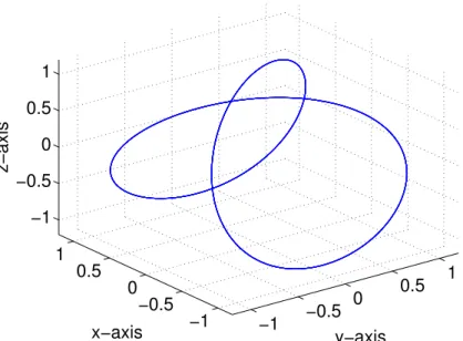
To understand this statement better let us assume a limit cycle attractor (a closed circuit). Its dimension is d = 1 so one should use a 3-dimensional space for re-construction. But one knows that it is possible to present a limit cycle also in 2 dimensions (fig. 1.3(a)). Why should one use 3 dimensions? The problem in 2 di-mensions are situations for which the reconstruction fails. Fig. 1.3(b) is no proper embedding because of its intersection. Looking at the situation of an embedding in 3 dimensions as required by Whitneys embedding theorem (fig. 1.4) one can see that an intersection is also possible. The crucial difference between both cases is its behaviour for small changes within the mapping: Imagine a small change in the mapping of fig. 1.3(b). The position of the intersection probably would change a bit but the intersection would still remain. Imagine the situation in 3 dimensions nearly every small change in the map would remove an intersection. The reason is the higher degree of freedom. And that is exactly the point: Whitneys theorem delivers the dimension in which the probabilty for an intersection falls down to zero.

Following approach can be also helpful for comprehension: Given two d1- and

d2-dimensional objects N and M placed in a dspace-dimensional space. Then the expected dimension dover of the overlap of both objects will be the sum of the object-dimensions subtracted by the space dimension (compare the limit cycle ex-ample):

(19)

1.2. Basic methods and definitions −1 −0.5 0 0.5 1 −1 −0.5 0 0.5 1 −1 −0.5 0 0.5 1 y−axis x−axis z−axis

Figure 1.4.:3-dimensional embedding of a Limit Cycle

For the situation of a self-intersection both objects become the same with dimension d1=d2 =d.

dover =2·d−dspace ⇒ dspace =2·d−dover (1.12) For an embedding there must not be any overlap. Hence the dimension of the overlapdover must be at least -1 or smaller:

dspace ≥2·d+1 (1.13) And finally one receives the equation provided by Whitneys embedding theorem.

Remark: Whitneys embedding theorem is powerful. It delivers important

infor-mation about the optimal dimension for reconstruction. Nevertheless it does not say that nearly every map can be used for Phase Space Reconstruction. The rea-son is that possible maps for reconstruction only depend on one component of the original attractor per definition. This means that the group of all possible recon-struction functions is only a vanishing small subset of all possible maps. Because of this strong restriction the probability to get an embedding could be smaller than 1, it could possibly also be 0. Also it is not clear if this additional restriction allows to change the mapping in a way that a false embedding become a true one. Hence

(20)

1.2. Basic methods and definitions it is important to keep in mind that Whitneys embedding theorem says something about the optimal dimension for reconstruction but it does not say anything about the probability that a reconstruction is an embedding!

1.2.10. False Nearest Neighbours

Whitneys embedding theorem delivers information about the optimal embedding dimension for a known attractor. But for measurement data the underlying system normally is not known. Therefore it is necessary to have additional tools for esti-mation of the embedding dimension. One possible solution is the so called "False-Nearest-Neighbours"-method. It bases on the idea that in the case of a too low dimensional embedding points will become direct neighbours which normally lie far away of each other. At the same time it is not possible to disperse real neigh-bours by using a too high embedding. To find the optimal embedding dimension d one has just to increment the embedding dimension starting with d = 1 and to test which points are neighbours in this actual embedding. Increasing the dimen-sion this number of neighbours will decrease: The false nearest neighbours will be reduced step by step. The optimal embedding dimension will be reached when the number of neighbours does not decrease anymore. This happens when only true nearest neighbours remain. Hence the attractor is embedded correctly.

Imagine a simple limit cycle. Using a too high embedding the attractor will still remain as limit cycle. Direct neighbours will remain as direct neighbours. Using only a one-dimensional embedding the attractor is projected on one line. One sides of the limit cycle will be folded on the other side. Therefore some points that were before on the opposite will now become neighbours.

This method is not used on the following pages. For analysing the reconstruction itself it is more useful to work with systems that are fully known. Anyhow it is important to be familiar with this method when applying it to real measurement data. A more detailed description concerning the optimal embedding dimension and a presentation of alternative methods can be found e.g. in [15] or [29].

(21)

1.2. Basic methods and definitions

1.2.11. Fractal dimension

Another important property of chaotic attractors is its fractal structure: Mostly they do not have an integral dimension. To understand this phenomena is it necessary to know how the dimension can be measured. Actually there are several measures for it. The best measure to understand its functionality is probably the box dimen-sion:

The box dimension takes a look at the scaling of an object. For that purpose the ob-ject is covered with boxes of the same edge lengthe. The relation between number of needed boxes Nand edge lengthedelivers the dimension Dof the object:

N(e) ∝e−D (1.14)

Choosinge big means that the resolution for analysing the attractor is low. Hence the definition of the Boxdimension uses the limit of e → 0 to make sure that every detail of the attractor is included in the result. After some transformations one gets the final formula:

DBox =−lim

e→0

ln(N(e))

ln(e) (1.15)

Another measure for the dimension is the so called information dimension DI. It bases on the same idea but works with probabilities. This definition delivers slightly different results (in general one can sayDI ≤DBox) but can also be used to describe fractal objects:

DI =−lim e→0 N(e) ∑ i=1 Pi(e)log(Pi(e)) log(e) with N(e)

∑

i=1 Pi(e) =1 (1.16)

Pi(e) is the probability to find a particle in the i-th space-area (the probability to find the particle in the whole space is 1).

Applying this concept on real time series also the numerical aspect becomes rele-vant. A limited set of points has dimension 0 by definition. Hence for a discrete dataset the dimension of the underlying attractor has to be approximated. One of

(22)

1.3. Some dynamical systems the numerical fastest ways is to calculate the correlation dimension d2. For this

dimension first the correlation integral has to be calculated:

C(e) = lim n→∞ 1 N n

∑

i=1 i−w

∑

j=1 H(e− |sj−si|) (1.17)

N is the number of summands and n is the number of used points. si stands for the i-th point of the used data in phase space. H is the Heaviside-function which has value 1 for inputs greater 0 and value 0 for all other inputs andwis the Theiler window which prevents counting of temporally correlated pairs (otherwise the cal-culated dimension will be too small [31]). Hence the correlation integral counts all pairs of points which have a distance smaller than e excluding pairs of points which were recorded approximately at the same time. Increasing e the number of pairs with a distance less than e will raise. The exponent of this raising is the correlation dimensiond2. C(e) ∝ed2 ⇒ d2= lim e,e0→0 lnC(e) C(e0 ln e e0 (1.18)

Numericallyd2will be derived by averagingd2for differenteor by fitting a straight line in a log-log-plot ofC(e)overe.

For the following work it is not important to get to know about other measures of fractal dimension and differences between them, hence I will only provide this basic information. Important to know is that the fractal dimension should only depend on the measure that is used and the attractor that is measured but not on its embedding. Hence the fractal dimension is such as the Lyapunov-exponents a good measure to test if an embedding was successful. For an correct embedding one should recieve the correct fractal dimension.

1.3. Some dynamical systems

For testing the functionality of reconstruction methods dynamical systems are needed. PSR is mostly applied to real measurement data. By contrast for testing purposes it is more helpful to use systems which are already known exactly. At the same

(23)

1.3. Some dynamical systems time most interesting systems are strange attractors. Hence I will use four different chaotic systems for presenting and comparing different reconstruction methods. The choice was done arbitrarily so any other attractor could also be used for the following parts.

1.3.1. Lorenz Attractor

−10

₀

10 −10

0

10

25

40 x

2

x

1

x

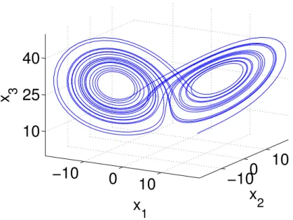
3

Figure 1.5.:Lorenz attractor

One of the first presented deterministic systems with chaotic behavior was a simple model for cellular convection invented by E. Lorenz [17]. Because of its low dimen-sionality and its - for a chaotic system - clear structure it is one of the most used examples for strange attractors. It is described by the following equations:

˙ x1 =σ(x2−x1) (1.19) ˙ x2 =−x1x3+rx1−x2 (1.20) ˙ x3 =x1x2−bx3 (1.21)

It becomes chaotic for certain parameters. One possible choice to produce chaotic behaviour which is used for all following examples isσ =10, r = 28 andb = 8/3

(24)

1.3. Some dynamical systems (fig. 1.5). For calculations a dataset was used with starting coordinates x1 = x2 =

x3 =5, timestep∆t=0.01 and length of 100000 points.

1.3.2. Rössler Attractor

−10

−5

0

5

10 −10

−5

0

5

10

0

5

10

15

20 x

1

x

2

x

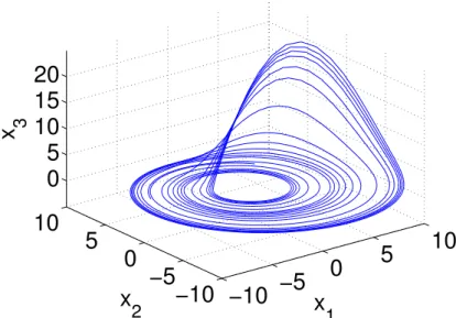
3

Figure 1.6.:Rössler attractor

The Lorenz attractor is simple for a chaotic system. However it is still too complex for some analysing methods. Therefore O.E. Rössler built a "model of a model" which should described the basic characteristics of the Lorenz system [21]. Instead of two spirals this system only contains one (fig. 1.6). For rebuilding the Lorenz system with the used parameters above Rössler got:

˙ x1 =−(x2+x3) (1.22) ˙ x2 =x1+0.2x2 (1.23) ˙ x3 =0.2+x3(x1−5.7) (1.24)

Another interesting property of the Rössler system is its mixture of chaotic and pe-riodic elements. Taking a look atx1orx2one will find functions with well defined

(25)

1.3. Some dynamical systems For my work I used a dataset with 100000 points, starting fromx1 =x2=4,x3=0

with timestep∆t=0.005.

1.3.3. Hénon Map

−1

−0.5

0

0.5

1 −0.2

0

0.2 y

x

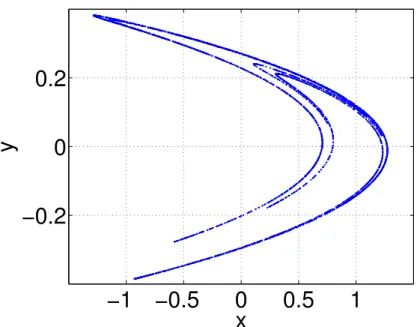
Figure 1.7.:Hénon attractor

Another ansatz to build up a simple chaotic system was done by Hénon [13]. The goal was to create a system which has similar properties compared to a Lorenz system but with simpler equations. This should reduce the amount of calcula-tions needed for a simulation. Therefore he tried to rebuild the Poincare map of a strange attractor instead of rebuilding the whole trajectories. The result was a two-dimensional discrete map with chaotic behaviour.

xn+1 =1+yn−ax2n (1.25)

yn+1 =bxn (1.26)

For a = 1.4 and b = 0.3 one gets a chaotic behaviour of this system. It is a good example to test the embedding of discrete systems and will be used in this way on the following pages.

(26)

1.3. Some dynamical systems The used dataset has 100000 points and starts fromx1 =0.7,x2=0.002.

1.3.4. Hyperrössler Attractor

−80 −40 0 40 −60 0 60 0 50 100 150 x 1 x 2 x 3 (a) x1,x2andx3 −80 −40 0 40 −60 0 60 10 30 50 x 1 x 2 x 4 (b) x1,x2andx4 Figure 1.8.:Hyperrössler attractor

Another class of chaotic systems are so called "hyperchaotic systems". In contra-diction to chaotic objects these systems contain at least two positive Lyapunov Ex-ponents. Hence hyperchaos is more chaotic and higher dimensional than chaotic systems. I will use a 4-dimensional hyperchaotic system invented by Rössler ([23], [22]) which is closely connected to the Rössler system introduced before.

˙ x1 =−x2−x3 (1.27) ˙ x2 =x1+0.25x2+x4 (1.28) ˙ x3 =3+x1x3 (1.29) ˙ x4 =−0.5x3+0.05x4 (1.30)

It is a good example for testing reconstructions with a more complex system. For that purpose I use a time series with 150000 points starting fromx1 =−10,x2 =−6,

(27)

1.4. Common methods for attractor reconstruction

1.4.1. Time Delay

Time delay was one of the first published methods for reconstruction (see [30] [20]) and is today the most frequently used one. One reason is probably that Floris Tak-ens could present very early a mathematical proof for its functionality. The other reason is its good usability: The additional coordinates are built using the original time series shifted in time with a delay τ. So the reconstructed systemv(t)has the structure:

v(t) = (x(t),x(t+τ),x(t+2τ), ...) (1.31) This is easy to handle for real measurement data because the reconstruction itself does not need any complex calculations. Instead the time series can be used directly. It also has the benefit that every dimension shows the same noise level.

Analysing discrete systems a reconstruction withτ =1 can also be interpreted very well because it follows the structure of discrete equations (xn+1 = f(xn)...). Hence one can say that it is some kind of natural reconstruction for these systems.

A disadvantage is the introduction of the parameterτ which has to be determined first. Takens embedding theorem says that nearly every τ gives a correct embed-ding but there are qualitative differences between these choices. Therefore it is necessary to calculate a proper delay τ first. At the same time the possibilities of optimizing the reconstruction is limited due to its definition. To get better results multiple time delays were introduced which make the reconstruction even more complex.

v(t) = (x(t),x(t+τ1),x(t+2τ2), ...) (1.32)

Nevertheless most papers published about attractor reconstruction are working only with time delay reconstruction and many papers are offering more efficient ways to calculate the correct embedding dimension and embedding delays.

(28)

1.4. Common methods for attractor reconstruction

1.4.2. Derivation

Another early published but not so well known method is a reconstruction using the derivatives of the original function (see [20]).

v(t) = (x(t),dx(t) dt ,

d2x(t)

dt2 , ...) (1.33)

Whereas most dynamical systems can be reconstructed very well using time delay coordinates there are also many cases for which the derivation method has some advantages. There are more numerical calculations necessary to get the new coor-dinates. In return this method needs only the reconstruction-dimension as input, no more values are introduced. This reconstruction gives often better results if the dynamical system bases on differential equations. In this cases the reconstruction has a similar structure as the original system and it is often possible to get a proper reconstruction in a lower dimension compared to time delay.

Hence time delay delivers correct reconstructions for nearly every system but often it is possible to get the same results in a lower dimension using other methods. The latter bears big advantages because a lower dimension also means better opportu-nities for working with the system.

Because of its structural similarity to differential equations the reconstructed di-mensions are often easier to identify with physical properties of a system and there-fore the reconstruction is often better to explain physically compared to a recon-struction with time delay.

On the other hand the derivation method has the disadvantage that the coordinates have different noise levels because of their different dependency on frequencies (high frequencies are amplified through derivation).

1.4.3. Integration

Reconstruction with integration is the opposite method of derivation.

v(t) = (x(t), t Z 0 x(t0)dt0, t Z 0   t0 Z 0 x(t00)dt00  dt0, ...) (1.34)

(29)

1.4. Common methods for attractor reconstruction It has similar pros and cons but does not work for real data as good as derivation. The reason is its high dependency on low frequent noise. This leads to the prob-lem that it only gives useful results in a combination with some moving average noise reduction or a similar technique. Some further discussions and explanations concerning integration reconstruction were done by Blasius et al. [3] and Gilmore [7].

1.4.4. Hilbert-Transformation

Hilbert Transformation is a method which is used to calculate the imaginary part of a signal. For this reason it is often applied in electronics to determine the complex impedance of an electrical system. This is its main application but it can also be used for reconstruction of other systems. Its behaviour can be described best taking a look at the frequency domain. There it is a rotation around the origin. Positive frequencies are rotated+π/2, negative ones−π/2.

v(t) = (x(t),IFFT(i·sign(ω)·FFT(x(t))) (1.35) (FFT = Fast Fourier Transform, IFFT = Inverse Fast Fourier Transform)

The method needs some numerical calculations to get the additional dimension but is easy to use because of the absence of selectable parameters. It also does not change the noise level and conserves the most important properties of the origi-nal time series. The big disadvantage is its limitation to only one additioorigi-nal re-construction dimension. So only a two-dimensional embedding is possible. This disqualifies the method for most situations. Anyhow it will help to understand the following ideas and will also be useful within the new methods presented in this work.

(30)

2. Look at the frequency-domain

2.1. Motivation

As we have seen above there are a few different methods for achieving the same goal. At the same time all these reconstructions have a quite different appearance in the time domain. Therefore the questions are:

• Why are all these methods producing similar results? (they are all offering proper embeddings)

• Are there more reconstructions that can be used?

• What are the requirements for a map that it can be used as a reconstruction? To answer this questions one needs to find a representation for which all these methods get a similar shape. The following pages will show that the frequency space is offering such a structure. There are primary two reasons that can motivate the use of the frequency space:

1. Using a time-series it is actually hard to imagine "where" information about the other dimensions is stored. Reconstruction appears in a way magical. Working in the frequency space the reconstruction process becomes more ev-ident: Instead of time one handles with frequencies and they are closely con-nected with motion on a circle. Therefore at least one single frequency has already some kind of two-dimensional interpretation. Using more frequen-cies a more-dimensional interpretation becomes more obvious.

For understanding of this motivation let us take the picture of a frequency as a motion on a circle: Intuition will predict that every frequency contained in one dimension should also be contained in all other dimensions. Intuitively

(31)

2.2. Common methods the only exception of this should be the non-generic case of a dimension that stands orthogonal on the flow.

2. Before Phase-Space-Reconstruction was invented the power spectrum of a function was used to determine chaotic behaviours. On its basis it was easier to detect signs for chaotic characteristics. But the power spectrum has the big disadvantage that the phase-information is neglected. Therefore it cannot be used for reconstruction and Takens began to use the time-series directly. But still it remains reasonable to work with frequencies for reconstruction. Hence the solution is to work with the fourier transform which uses a frequency-representation without neglecting the phases.

Most likely this argumentations are easy to challenge but one has to keep in mind that these are only motivations. They should be understood as indications for the following pages.

2.2. Common methods

2.2.1. Time Delay

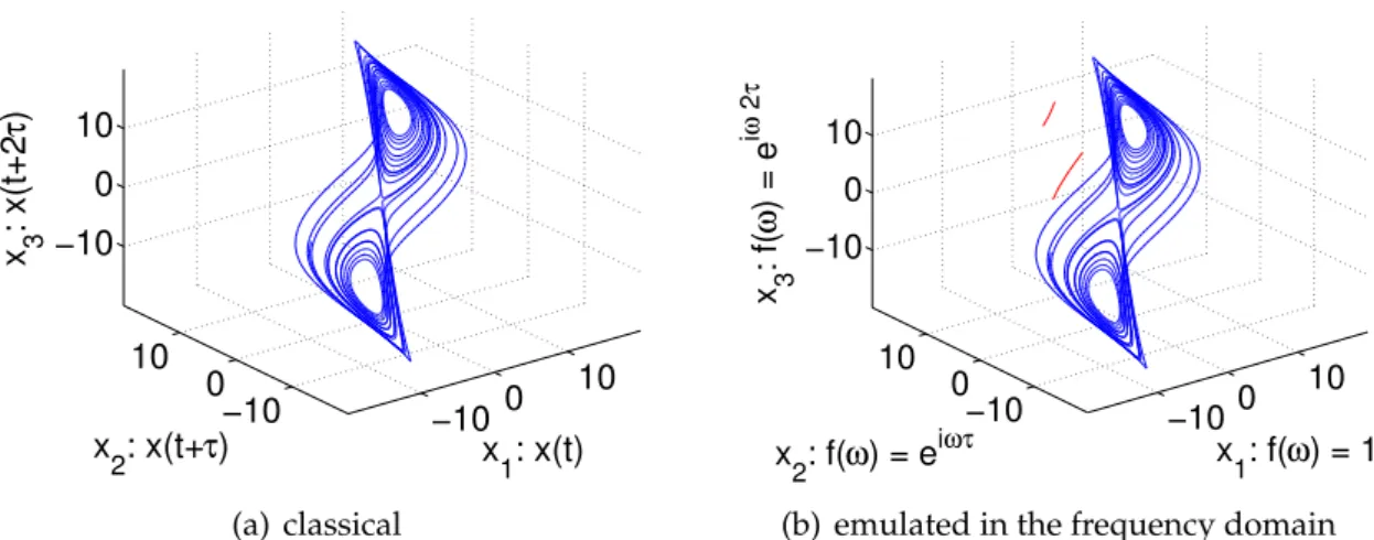
Using the Fourier-transformation a time delay nτ in the time domain becomes a multiplication with the exponential functioneiωnτ _{in the frequency domain.}

xn+1(t) = x(t+nτ) ⇒ x˜n+1(ω) = x˜(ω)·eiωnτ (2.1) It has to be remarked that this representation is valid for the case of infinite time series. For real data one has to deal with finite data. Also the numerical ways of getting the additional coordinates are completely different. For the classical method one has only to shift the data. In the new case one has to transform the data to the frequency domain, multiply it with a frequency-depending factor and have to transform it back to the time domain. So it is necessary to compare both realizations to test the assumption that both ways producing the same result.

Figure 2.1 shows the example of a Lorenz attractor [17] reconstructed with both re-alizations. As expected both ways provide the same results with only two small

(32)

2.2. Common methods −10 0 10 −10 0 10 −10 0 10 x 1: x(t) x 2: x(t+τ) x 3 : x(t+2 τ ) (a) classical −10 0 10 −10 0 10 −10 0 10 x 1: f(ω) = 1 x 2: f(ω) = e iωτ x 3 : f( ω ) = e i ω 2 τ

(b) emulated in the frequency domain

Figure 2.1.:Time-Delay reconstruction of a lorenz system using the x-axis: Comparison between the classical method shifting the data (2.1(a)) and the emulated version in frequency-space using a multiplication with exp(iωnτ)(2.1(b)).

exceptions (marked red, fig. 2.1(b)). These wrong trajectories are caused by bound-ary effects due to the finiteness of the time series. Equation 2.3 shows the difference of the finite calculation. Because of the limited dataset one gets some additional terms which are rising with time-shiftτ:

n

∑

t=0 x(t+τ)e−iωt = n+τ

∑

t=τ x(t)e−iω(t−τ) _(2.2) = n

∑

t=0 x(t)e−iω(t−τ)₊ n+τ

∑

t=n+1 x(t)e−iω(t−τ) ₋ τ−1

∑

t=0 x(t)e−iω(t−τ) | {z }

difference to continuous case

One could use now the exact formula but this would gain the complexity of further calculations. Instead it is more practicable to keep this problem in mind and deal with it.

In case of time delay both lines have the lengthτand can be easily removed just cut-ting the ends of the reconstructed datasets (in the classical case we also have to cut the ends of our datasets because of the shifting). Finally after cutting one receives two reconstructed datasets with the same length and values. So exactly the same reconstruction is received with the continuous formula using some corrections at the end.

(33)

2.2. Common methods One remark has to be made at this stage: The result above is only valid if no infor-mation is lost due to the Fourier Transforinfor-mation. This induces that the sampling rate fulfilled the Nyquist-Shannon sampling condition!

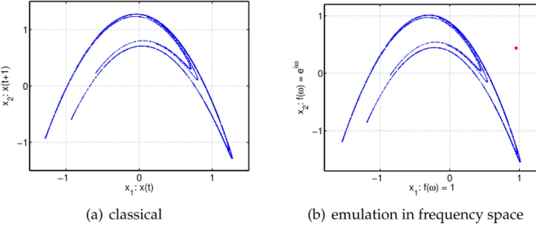
A similar result is found looking at the example of a discrete Hénon map (fig. 2.2).

−1 0 1 −1 0 1 x2 : x(t+1) x₁: x(t) (a) classical −1 0 1 −1 0 1 x₁: f(ω) = 1 x2 : f( ω ) = e i ω

(b) emulation in frequency space

Figure 2.2.:Time-Delay reconstruction of a discrete hénon map using the x-axis: Com-parison between classical method (2.2(a)) and emulation in frequency space (2.2(b)). The used delay isτ=1.

The classical method produces nearly the same result compared to the reconstruc-tion in fourier space. Also both reconstrucreconstruc-tions are similar to the original system. As in the example of Lorenz system the reconstruction delivers one wrong point (only one point because ofτ =1) marked red in fig. 2.2(b).

Another visible but not fundamental difference is the absolute position of the at-tractor. This is caused by the syntax I used for reconstruction in frequency space: Using time-delay the component for ω = 0 has normally to be multiplied with exp(iτ·0) = 1. My explicit realization in frequency space instead sets this compo-nent to zero. The reason for this choice is to prevent singularities forω = 0 which are e.g. produced by integration reconstruction in chapter 2.2.3. Actually this con-stant shift does not infect the quality of an embedding. Hence it does not matter if this part is removed or not.

2.2.2. Derivation

Derivation of a function in time domain becomes a multiplication with the function f1(ω) =iωin frequency domain. Hence the transformation gets the structure:

(34)

2.2. Common methods

xn+1(t) =

dnx(t)

dtn ⇒ x˜n+1(ω) = x˜(ω)·(iω)

n _(2.3)

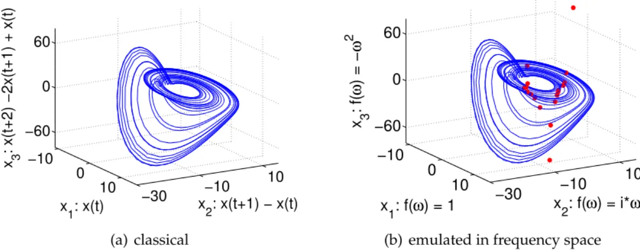
Fig.2.3 compares the classical derivation reconstruction of a Rössler system [21] with its emulation in frequency space.

−10 0 10 −30 −10 10 −60 0 60 x₂: x(t+1) − x(t) x 1: x(t) x 3 : x(t+2) −2x(t+1) + x(t) (a) classical −10 0 10 −30 −10 10 −60 0 60 x 2: f(ω) = i*ω x 1: f(ω) = 1 x 3 : f( ω ) = − ω 2

(b) emulated in frequency space

Figure 2.3.:derivation reconstruction of a Rössler attractor using the x-axis: Compar-ison between classical realization (2.3(a)) and its idealized counterpart in frequency space (2.3(a)).

Also for derivation reconstruction one receives similar results for both realizations. But compared to the results of time-delay the differences are bigger: In contrast to time-delay the disturbances are not primary produced due to the finiteness of the used time series. More problematic becomes the discretization of data: For discrete data it is not possible to calculate its derivation in the time domain. Instead the difference between two following points is used as approximation. Coevally the counterpart of an exact derivation was used in frequency space for reconstruction. In case of continuous data the result would be the same but for discrete data the operations differ. Nevertheless the results are still comparable. The disturbances in the alternative reconstruction are only situated at beginning and end of the time series. Therefore it is easy to remove these parts.

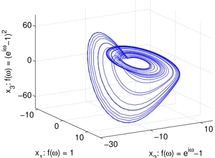
Alternatively it is also possible to use the exact counterpart of the used deviation instead of the derivation (eq. 2.4).

(35)

2.2. Common methods x2(t) = x(t+dt)−x(t) dt ⇒ x˜n+1(ω) = x˜(ω)· eiωdt₋₁ dt !n (2.4)

Fig. 2.4 shows the result applying this accurate emulation of the used reconstruc-tion. The difference to the classical case (fig. 2.3(a)) are two wrong points caused again by boundary effects due to a delay ofτ =1 (beyond the plotting range of the figure). −10 0 10 −30 −10 10 −60 0 60 x 2: f(ω) = e iω −1 x 1: f(ω) = 1 x 3 : f( ω ) = (e i ω −1) 2

Figure 2.4.: alternative derivation reconstruction of a Rösslersystem using the x-axis: exact emulation of the classical reconstruction reconstruction (2.3(a)).

Because of its easier handling only equation 2.3 will be used for the following ex-amples. But there is no problem to use also the exact transformed equation. Both methods can be applied in the same way and the choice only depends on the re-quirements the experimentalist has for reconstruction.

2.2.3. Integration

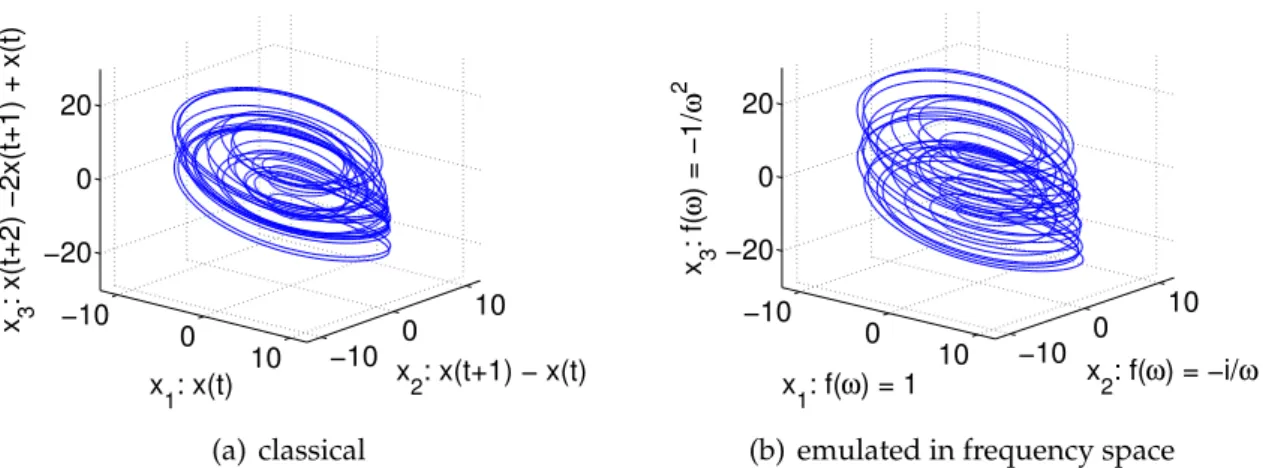
Without taking notice of the mentioned problems of integration reconstruction (chap-ter 1.4.3) the integration reconstruction becomes a division with iω in frequency space. As the counterpart of derivation reconstruction this result gets clear imme-diately.

(36)

2.2. Common methods x2(t) = t Z 0 x(t0)dt0 ⇒ x˜n+1(ω) = x˜(ω)· 1 (iω)n (2.5)

As explained before this result normally cannot be applied directly on a time series because of its magnification of low frequent disturbances. However the aim at this point is to understand the reconstruction structurally and not to find the practically most valuable method. This can be reached best by comparing first the idealised and most simplified reconstruction version before taking a look at its practical is-sues. Hence 2.5 gives a comparison between the skeletal structures of classical in-tegration reconstruction and its emulation in frequency space.

−10 0 10 −10 0 10 −20 0 20 x 2: x(t+1) − x(t) x 1: x(t) x 3 : x(t+2) −2x(t+1) + x(t) (a) classical −10 0 10 −10 0 10 −20 0 20 x 2: f(ω) = −i/ω x 1: f(ω) = 1 x 3 : f( ω ) = −1/ ω 2

(b) emulated in frequency space

Figure 2.5.: reconstruction with integration of a Rössler attractor using the x-component: Comparison of the standard method (2.5(a)) with its emulated counterpart (2.5(a)) and without additional filtering.

As one can see the result does not embed the dynamics correctly. But at the same time it is noticeable that both methods deliver similar results. Analogue to deriva-tion reconstrucderiva-tion the emulated result differs more of its prototype as e.g. for time-delay. And as for derivation reconstruction this error is caused by the discretization of data: Because of this condition there is no real integration in the time domain. Instead all points are summed up. This difference leads to the differences in the reconstruction. It has also to be remarked that there is a small discrepancy between the equation shown above and the used equation in frequency space: As already denoted in chapter 2.2.1 I added a small change to the sourcecode that was used for emulation: The component for a vanishing frequency is set to zero. This becomes here important because otherwise one would get a singularity for ω =0. Coevally

(37)

2.2. Common methods this fact is closely connected to the problems using integration reconstruction: Also frequencies close to zero are amplified too much. In the presentet case this does not affect the first reconstructed component but leads to a divergency in the second reconstructed dimension because of its quadratical dependency onω.

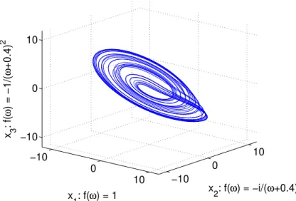
Classically this problem is solved by applying a moving average filter to the data. Working in the frequency space this can be done much easier just by introducing a small offset. Figure 2.6 shows the result using this modification.

−10 0 10 −10 0 10 −10 0 10 x 2: f(ω) = −i/(ω+0.4) x₁: f(ω) = 1 x 3 : f( ω ) = −1/( ω +0.4) 2

Figure 2.6.:optimized integration reconstruction of a Rössler system: Lowfrequent dis-turbances are neglected by introduction of a small offset.

The emerged embedding is not the best but all topological properties are mapped correctly. Also it is easy to identify the Rösslersystem. Hence this reconstruction gives a first example for the advantages of reconstruction in the frequency domain: It is easier to modify reconstructions and to optimize them for a given dataset.

2.2.4. Hilbert-Transformation

In the case of the Hilbert transformation no comparison is necessary: The recon-struction is already done in the frequency domain. At the same time the structure in the frequency domain is the simplest one of all presented reconstructions:

˜

(38)

2.3. Generalization Worth mentioning is its strong affinity to reconstruction with derivation or inte-gration. The only difference is that derivation and integration are working with the frequency as a weighting function instead of only using its sign. This fortifies the relevance of Hilbert-Transformation as a reconstruction that is reduced to the essential. −10 0 10 −10 0 10 x 2 : f( ω ) = i x 1: f(ω) = 1

Figure 2.7.:Hilbert Reconstruction of a Rössler system using the x-component

2.3. Generalization

2.3.1. Overview

I showed that it is possible to emulate all presented reconstructions in frequency space. Considering the mentioned limitations the results of classical and emulated technics delivering nearly the same results. Hence in the following the emulations will be used as proper replacements for the classical methods. The next step is to compare them with each other to find similarities. For this purpose table 2.1 provides an overview about the presented methods.

As already known there are not many similarities between these methods looking at the time domain: It is nearly impossible to identify a general structure for all reconstructions. Taking a look at the frequency space one will find a much more

(39)

2.3. Generalization

method time domain frequency domain

Time Delay xn+1(t) = x(t+nτ) xñ+1(ω) = x˜(ω)·eiωnτ Derivation x2(t) = x˙(t), x3(t) = x¨(t),... xñ+1(ω) = x˜(ω)·(iω)n Integration x2(t) = t R 0 x(t0)dt0,... xñ+1(ω) = x˜(ω)· (iω1)n Hilbert x2(t) = IFFT(i·sign(ω)·x˜(ω)) x˜2(ω) = x˜(ω)·i·sign(ω) Table 2.1.:Comparison of most common reconstruction methods displayed in time and frequency domain.

structured situation: All reconstructions can be described as a product between original time-series and a frequency-depending function f(ω).

˜

xn(ω) = x˜(ω)· fn(ω) (2.7) That means that one needs only the original time seriesx(ω)and n different recon-struction functions fn(ω) (one function per embedding dimension) to reconstruct the attractor. Hence every reconstructed dimension provides the frequency struc-ture of the original time series with some variations in phase and amplitude. This clear structure of reconstruction leads to the questions of the beginning: Are there more possible reconstruction functions? Is there perhaps a whole class of functions which can be used for reconstruction? What are the requirements for f(ω) to be a proper reconstruction function?

2.3.2. Requirements on the reconstruction functions

f

n

(

ω

)

To get information about the properties of the reconstruction functions fn(ω) it is necessary to think about the requirements for a good reconstruction. One important requirement is that all reconstructed dimensions must be real-valued. Because we are working with complex values in the frequency domain a real-valued output leads to restrictions for the reconstruction function:

(40)

2.3. Generalization x(t) = √1 2π +∞ Z −∞ (a(ω) +ib(ω))e−iωtdω x(t),a(ω),b(ω) ∈ R ⇒ ∀t∈ R: 0= +∞ Z −∞ b(ω)cos(ωt)−a(ω)sin(ωt)dω ⇒ a(ω) = a(−ω) ∧ b(ω) =−b(−ω) (2.8)

This means that the Fourier transformed of a real valued time series has the prop-erty: ˜x(ω) = x˜(−ω). The function itself and its complex conjugated of the negative frequency needs to be the same.

In the case of a reconstructed dimension the Fourier transformed is a multiplication of the reconstruction function and the Fourier transform of the original time series

fn(ω)x˜(ω):

fn(ω)x˜(ω) =! fn(−ω)x˜(−ω) ∧ x˜(ω) = x˜(−ω) (2.9) Hence one property of the reconstruction functions fn(ω)is:

fn(ω) = fn(−ω) (2.10)

Another requirement is the linear independency of all reconstruction functions:

f1(ω)...fn(ω)linearly independent (2.11) This is necessary to prevent same reconstruction results for different reconstruction dimensions. In phase space all components needs to be linearly independent. Oth-erwise the embedding will be flat and could also be presented in less dimensions. Hence in this case at least one dimension must be redundant. Because of the linear-ity of Fourier transformation this requirement can directly be adopted to frequency space.

(41)

2.3. Generalization Besides these two obvious requirements there must be even more. In the following part I will present a third requirement in a heuristic way. An accurate description of this part would be very useful and should be aimed at future investigations. Using the limitations above fn(ω) can still be nearly everything. So it would be also possible to use e.g. fn(ω) = random (fig. 2.8) or to use functions which are discontinuous at every point. As shown in fig. 2.8 for the random case this obvi-ously does not work. In fact this would mean that one could produce every result one wants to have just by choosing the reconstruction functions. It would be pos-sible to eliminate the original signal nearly completely. This cannot deliver proper embeddings! −10 0 10 −10 0 10 −10 0 10 x 1: f(ω) = 1 x 2: f(ω) = random x 3 : f( ω ) = random

Figure 2.8.:Failed reconstruction of a Rössler system using random numbers as recon-struction functions

For an accurate reconstruction it is necessary to conserve the basic elements of the original system. The ideal reconstruction changes the accent within the time series but it does not add or remove information. The reconstruction functions them-selves should be neutral. Mathematical imprecise this means that the functions fn(ω) have to be smooth. And in fact all classical functions are continuous and differentiable inωexcept the pointω =0.

So a good but perhaps not necessary postulation should be the continuity of fn(ω).

(42)

2.3. Generalization Also a stronger postulation could be necessary. A continuous function could also be able to "overwrite" the frequency information of the original system if the recon-struction function moves very fast in the order of magnitude of the original data. The reconstruction can also be understood as some kind of filtering1(effectively fil-tering has the same structure in frequency domain as the propagated reconstruction in equation 2.7).

Filtering means that some parts are highlighted while some other parts are atten-uated. As more loading is done as more information of the original signal is lost. Without filtering we have the case f(ω) = 1 and we do not get any reconstruc-tion. At the same time too aggressive filtering as e.g. f(ω) = random removes the original information completely. Hence a good reconstruction needs to find a good balance between both extremes. Under this point of view it could be better to postulate slowly varying functions fn(ω)(eq. 2.13) instead of only claim continuity (eq. 2.12).

fn(ω)slowly varying (2.13)

2.3.3. Syntax declaration

Before taking a look at some examples it is important to fix the used syntax for all reconstruction functions fn(ω). Chapter 2.3.2 showed that there is an explicit re-lationship between f(ω) and its negative counterpart f(−ω)(equation 2.10). That means that one only needs to define the reconstruction functions for positive fre-quenciesω ≥0. Then the negative part is defined automatically.

So far all shown reconstruction functions were already fulfilling equation 2.10 in the presented structure. Anyhow there are many situations were the full function for the whole frequency-spectrum is more complex as the same function defined only for positive frequencies. For example the Hilbert transformation has f(ω) = i·sign(ω). Describing the behaviour only for positive frequencies one can write

f(ω) = i.

1_{Here the notion "Filter" is used in the physical meaning, not in the mathematical. Mathematically}

a filter discriminates more: Objects are either removed or left unaltered. For reconstruction is this behaviour too strong: information of the system is changed significantly. In contrast a physical filter only modifies the phases and amplitudes of different frequencies. Therefore it changes the signal quite less.

(43)

2.3. Generalization Another example is an integration with a small offseta. The reconstruction-function for the full space (2.14, left) is much more complex compared to the function only written for positive frequencies (2.14, right):

f(ω) = 1

i·sign(ω)(|ω|+a) ⇔ f(ω) = 1

i(ω+a) (2.14) A simpler structure allows to capture the kind of reconstruction more easily. At the same time no information is lost. For example in the last case the relationship to unmodified integration is much better to detect in the right declaration. From my point of view the higher complexity of the left formula is only confusing. Also under knowledge of the symmetry in frequency space the left equation can be de-rived easily of the right one if needed. Therefore in the following examples the reconstruction function will be only defined for positive frequencies!

So keep in mind: f(ω) is defined only forω ≥ 0! The behaviour for negative frequencies can be derived using equation 2.10.

2.3.4. Some examples

Using this new reconstruction method one gets a whole bunch of possible recon-struction functions. One interesting option is to change well known reconrecon-structions slightly. Instead of f(ω) = iω (derivation) one can use f(ω) = ω or f(ω) = i

√

ω.

Both changes can help to produce a reconstruction similar to derivation reconstruc-tion but with less dependency on high-frequent parts.

In the case of a 4-dimensional reconstruction of a signal one gets with derivation reconstruction terms up to the order ofω3:

f1(ω) =1 f2(ω) = iω f3(ω) =−ω2 f4(ω) = −iω3 (2.15) This means that this reconstruction is already useless for experimental data with low amount of noise. As a solution following reconstructions could be used:

(44)

2.3. Generalization This reconstruction can be interpreted as a standard derivation reconstruction which is stretched by doubling each reconstruction dimension with a Hilbert transforma-tion. Another choice would be:

f1(ω) = 1 f2(ω) = i √

ω f3(ω) = −ω f4(ω) = −iω3/2 (2.17) In this case the classical raise in orders ofω for each step is still conserved. Instead the raising order itself is decreased from 1 to 1/2. Both cases reduce the highest order in ω strongly. Which method should be used depends on which properties should be conserved. Should the reconstruction use only integral orders of mag-nitude (eq. 2.16)? Or is it more important that for every dimension the order of magnitude inωis increased (eq. 2.17)? Furthermore it is still possible to create own reconstructions and to make stronger reductions.

Another idea is to use functions with a low gradient for high frequencies as e.g. arctan(ω) or log(ω +1). So one could use a derivation reconstruction and just replaceωwith log(ω+1).

To show that all these choices delivering useful results I will present some plots of these customized reconstructions applied to Lorenz- and Rössler-systems:

−20 0 20 −20 0 20 −40 0 40 x 2: f(ω) = ω 0.5 x 1: f(ω) = 1 x 3 : f( ω ) = i ω

(a) Lorenz attractor

−10 0 10 −10 0 10 −20 0 20 x 2: f(ω) = ω 0.5 x 1: f(ω) = 1 x 3 : f( ω ) = i ω (b) Rössler atractor

Figure 2.9.: Customized reconstructions using a modified derivation reconstruction with weakened frequency dependence