VU UNIVERSITY AMSTERDAM
BMI PAPER
Social Networking Analytics
Abstract
In recent years, the online community has moved a step further in connecting people. Social Networking was born to enable people to share more, on social and professional level. Due to its potential, significant scientific and technological efforts are made to better understand, control and extend this phenomenon. The public accessibility of web-based social networks stimulated extensive research in this domain. Understanding how networks grow and change, and being able to predict their behavior, contributes to the evolution of other domains such as business, education, social, biology, fraud detection, criminal investigation etc. This paper surveys fundamental concepts of social networking analytics as well as a set of established models for the problem of link prediction. Two case studies are supporting the paper: the first study treats the problem of influential behavior by measurements of centrality and power; the second study compares the accuracy of three classification algorithms for a case of co-authorship link prediction.
Author: Elena Pupazan Supervisor: Dr. Sandjai Bhulai
2
Preface
This paper is written as a compulsory part of the Business Mathematics & Informatics master program at the VU University Amsterdam. The purpose of the paper is to engage the student to research on a subject of his choice as extension to the knowledge acquired during the study. The addressed problem should be business related and a computer science and/or mathematical method should be used to find answers. During the project the student is supervised by a staff member who is specialized in the chose subject.
The topic of this paper is Social Networking Analytics, with focus on underlying concepts of the discipline, behavior aspects in social networks and link prediction modeling. The choice of the topic is reasoned by the personal interest in the phenomenon of Social Networking as well as in Predictive Analytics. The core message of the paper is the significant role of social networking analytics in various activity domains.
The paper is structure in seven chapters: Chapters 1 introduces the studied topic; Chapter 2 presents briefly the evolution of Social Networking and Social Networking Analytics; in Chapter 3 there are introduced fundamental concepts and metrics in Social Networking Analytics; Chapter 4 focuses on behavioral aspects of Social Networking, introducing a set of established link prediction models. The presented theoretical aspect are supported and extended by two case studies: Chapter 5 presents a study of influence within the Bernard & Killworth fraternity, over a determined period of time. The analysis is based on measurements of centrality and power, using the UCINET 6 technology. Chapter 6 proposes a comparison of accuracy of three learning algorithms: Support Vector Machine, K-Nearest Neighbor and Naïve Bayes for the link prediction problem in the DBLP co-authorship community. The specific of this study is the particular set of features applied in learning. Chapter 7 presents the conclusions of the conducted research in Social Networking Analytics.
I would like to thank my supervisor, Dr. Sandjai Bhulai, for his support and guidance in scoping and writing this paper.
Elena Pupazan Amsterdam, 2011
3
Table of contents
Abstract ... 1
Preface ... 2
1.
Introduction ... 4
2.
Evolution of Social Network Analytics ... 5
3.
Basic concepts in Social Networking ... 6
3.1 Graph theory ...7
3.2 Sociomatrices ...9
3.2 Measures in Social Networking ... 11
4.
Behaviour and Dynamics in Social Networks ... 23
4.1 Structural Balance of Social Networks ... 24
4.2 Link Prediction Models ... 26
4.2.1 Mathematical framework ... 26
4.2.2 Models based on node similarity ... 27
4.2.3 Models based on topological patterns ... 29
4.2.4 Models based on a probabilistic model ... 33
4.2.5 Conclusion ... 38
5.
CASE STUDY 1: Influence in Virtual Communities... 39
5.1 Data ... 40
5.2 Approach... 42
5.3 Results and Discussions ... 43
5.4 Conclusions ... 56
6.
CASE STUDY 2: Co-authorship Link Prediction ... 57
6.1 Data ... 57
6.2 Approach... 58
6.2 Results and Discussions ... 60
6.3 Conclusions ... 62
7.
Conclusions... 63
4
1. Introduction
Before Twitter, there was Facebook, before Facebook there was Flickr, before Flickr there was MySpace and so on. All these virtual communities brought people together from all sides of the world, encouraging social and professional interaction.
As the interest of individual in virtual social networking grows, more scientific attention is given to them. Systems are being developed for understanding how and who acts in such social networks. These are tracking every possible social networking activity: usage, topics, who interact with who, for how long, user specific interests etc. Social Networking Analytics (SNA) is the discipline incorporating such scientific interests, arose from a long standing practice called Social Network Analysis. Social scientists trained in the latter study how people and groups are connected to each other (similar to the “Six Degrees of Separation” game). After the introduction of virtual social networks, it was a natural progression to apply the learned concepts and practices in the internet world.
Due to the high popularity and flexibility of social networking sites, companies had to develop unique strategies of reaching customers through those channels. Many SNA services and applications are today cloud-based and offer organizations various ways to track and interpret customer activity on such sites.
Understanding how people interact and what they are interested in will not only help the sales sector, but also the areas of marketing, HRM, CRM and so on. Some of the benefits of SNA are the abilities to better segment customers and estimate customer life cycles. A company is able to better see the key influencers who are leading the conversations. From there, an untapped pool of potential customers can be found and reached. Most of the services available now are offered at reasonably low costs. When leveraged by the right people and in the right way, businesses have the potential to grow and expand in a way that wasn’t thought possible just a few years ago.
From a CRM perspective, being able to interact with customers on a personal level, inways that are comfortable for them, will strengthen those customer relationships and make them last. Being proactive does not go unnoticed by customers, when their problems are recognized and fixed in a timely manner, these customers are more likely to continue using the company products or services. SNA should not be used to replace a customer service or the CRM program, it should be seen and used as an extension to the overall system.
As networks continue to increase in numbers and technology becomes more advanced, even more tools for social networking analytics will come on the market, each delving deeper into the system and offering more and more insight. If used correctly, social networking analytics may be a key tool in helping an organization to find and connect to the right markets and audiences, on a personal level.
5
2. Evolution of Social Network Analytics
Due to the recent globalization of the commercial environment and the impact of the new technologies,the analysis of social networks represents a major interest. This rather new area of research grew out of social and exact sciences, computers supporting today modeling and complex mathematical calculations, previously impossible. The analysis of social networks is driven by business and social interests, combining various academic fields.
The term social networks was used for the first time in 1950 in sociometrics, the science that seeks to obtain data on social behavior and to analyze it. The latter incorporation of mathematical tools and computing triggered the evolution of Social Network Analysis and Analytics.
The mathematical basis of SNA arose out of the fields of graph theory, statistical and probability theory, game theory as well as algebraic models. In fact, it was from these theories, especially graphs, that the Internet and various virtual networking concepts were derived.
Networks are generally studied based on the participants and their actions in the network, with little or no emphasis on the relationships. Particularly, in Social Networking and SNA thetypeand theforms of relationships between the network members are fundamental.
Social networking data comes today in many forms: blogs (Blogger, LiveJournal), micro-blogs (Twitter, FMyLife), social networking (Facebook, LinkedIn), wiki sites (Wikipedia, Wetpaint), social bookmarking (Delicious, CiteULike), social news (Digg, Mixx), reviews (ePinions, Yelp), and multimedia sharing (Flickr, Youtube).
Online social networking represents a fundamental shift of how information is being produced, transferred and consumed. User generated content, in any data form, establishes a connection between producers and consumers of information. For consumers, the abundance of share data and opinions is a support in making more informed decisions.
SNA is applicable in various domains and fields: organizational behavior, terrorist networking, political and economic systems, inter-relationships between banks and companies, social influence, educational systems and many others. Some of the current interests and challenges in the discipline of SNA are:
Collecting massive amounts of data and preventing information overload for the users
Extracting and modeling temporal patterns of information growth and fade over time
Correcting effects and biases generated by incomplete or missing data
Handling unreliable or conflicting information
Classification and tracking of topics
Identification of topic relevance
Predicting and identifying emerging or popular topics
Detecting, quantifying and maximizing the individuals influence
Determining implicit links between users
Understanding of sentiment flow through networks and polarization
This paper treats fundamental concepts in social networking and addresses in particular two topics of interest in SNA: influence and link prediction.
6
3. Basic concepts in Social Networking
A social network can be defined as a finite set of actors and their relationships. This is a simple and direct concept, allowing everyone to understand the social network according to the complete data and the connectivity of a considered network. This definitions does not say much though over the types of relationships of certain groups (i. e. the number of times they take part in the same programs or activities).
Fig.1 Social Network
An actor is the social entity who participates in a certain network and who is able to act and form connections with other actors. It could be an individual, a corporation or a social body. Examples of actors could be the students in a classroom, the departments in a company, the states of a federation, the web sites of a given business sector, the member nations of the UN etc. When all the actors of a network are of the same type, the network is calledmonomodal. But there are cases in which there are different actors in a network. In a multi-agent system, the actor is called anagent.
A link between two actors in a social network is called aconnection. It is defined by some type of relationship between these actors, depending on the type ofsociety. Between companies, the connection could be a business contract of supply, between people in a company, it could be the hierarchic relationship, if considering the organizational structure, or it could be the sending of e-mails in a network of relationships between friends. Other examples include the relationships of friendship or respect between students in a classroom, the biological relationships (in a family), the associations of members to clubs, the diplomatic relationships between countries etc. In the graph theory section presented later in the paper it will be shown that connections may have a value as well as a direction. To study networks of various relationships in an objective way, models need to be created to represent them. There are threenotationscurrently in use in the social network analysis:
Graph Theory – the most common model for visual representation, it is graph based
Sociometrics – proposes matrices representation, also called sociomatrices
Algebraic – proposes algebraic notations for specific cases, especially for multiple relationships (Wasserman [1994])
Each notation scheme has different applications and will enable different developments and analyses. Further, this chapter presents concepts and notations used for representations with graphs and sociomatrices. The combination of these two techniques has helped significantly the evolution of social network analysis.
7
3.1
Graph theory
The Graph theory has been widely used in analyses of social networks due to its representational capacity and simplicity. Basically, the graph consists of nodes (n) and of connections (l) which connect the nodes. In social networks the representation by graphs is also called sociogram, where the nodes are the actors or events and the lines of connection establish the set of relationships in a two dimensional drawing.
Dyad is the simplest network, composed of only two nodes, that may be connected or not. If connected, this represents a property of the pair.
Fig. 2 Example of Dyad
Triad is a network formed by three nodes and the possible connections between them. The triad brings some important concepts into question, such as the equilibrium and the transitivity which are presented later on. There are maximum three dyads in a triad. In business relationships, this can be an important factor because if Node 1 has a relationship with Node 2, and they in turn with Node 3, there is a possible path through Node 2 and on to Node 1 to make transactions with Node 3.
Fig. 3 Example of Triad
Group. A group can be defined as the set of all the nodes and their connections, considering a limit defined for the group. For example, the set of nations belonging to the UN and the business transactions could define a group, with the links between the countries being the connections between them. The definition of the limit is important to be able to study the group. Of course the students in one classroom have relationships of friendship with others outside of this limit, just as nations may have business relationships with countries outside the UN. But for the purposes of analysis of the social networks, the definition of the limits defines the group.
Subgroup. Within a group, there are many dyads and triads, but the concept of small sets of nodes can be extended within a group to be asubgroup. This can be very important in the study of complex and large social networks with the analysis of specific subgroups defined within the group.
Relationship. The set of connections of a given type defines the relationship found in the social network under analysis. Whereas a connection is only between two actors or nodes, the relationship is defined for the whole set of connections. Thus, we can talk about social relationships, business relationships, educational relationships etc. In the social network, there may be a connection between two actors (a situation where often the variable is set to “1” in a table or matrix), or there is none (represented with a “0”).
8
There are also relationships which imply values, when there is a connection and this connection can be attributed with a value (i.e. the financial worth of the business relationships between companies). The social networks where values are also involved, have a greater degree of complexity. This also due to the possibility of direction within a graph (i.e. a given company buys from another, but sells nothing to it).
Adopting next some of the nomenclatures, as in Wasserman and Faust [1994], the actors of a network will be noted n, and the set of actors as N. The connections of a network will have notation l, and the set of connections will be L. Thus, a network of “f” actors and of “h” connections will have the sets of actors and of connections defined respectively by: = , , … , and = { , , … , }.
As the connection is always between two actors, then the connection defines a pair of actors (or dyad). If saying that a connection l1 refers to the connection between actors n2 and n5, then we can write: =< , >.
Up to this point it has been defined a connection between two actors without being concerned about the type of relationship. Many of these connections are non-directional, meaning that a connection between two actors is established and that the relationship is not in any specific direction. For example, marriage establishes a relationship which is non-directional as it is not possible for a member to be married to another and that the inverse is not also true. If considering that the type of connection between companies to be the existence or otherwise of a contract, such a connection is non-directional.
A directional connection is that which represents a connection which goes from an actor (origin) and ends at another (destination). For example, if making an analysis which considers purchases and sales between companies of a network, there will be a direction in the connections. The image below (Figure 4) exemplifies the concept. In the first case, the direction of the arrow shows that actor 1 sells to actor 2; in the second, actor 2 sells to 1, and in the last case, the graph represents that actor 1 sells to actor 2 and also that actor 2 sells to actor 1.
Fig. 4 Directional connection in graphs
So if a connectionl1refers to the directional connection of actorn2to actorn5: = < → >. For a network with the number of actors equal to“f”, the maximum numberlmaxof connections in a non-directional graph can be written using the expression:
= ( −1) 2
In other words, for two actors the maximum is one connection, for three the maximum is three, for four, it’s six, and so on, as shown in Figure 5 below:
9
Fig. 5 Maximum number of connections in non-directional graphs
Indirectionalgraphs, the maximum number of connections (arrows) between two actors is two arrows (one in each direction), for three actors the maximum is six, and so on. The expression which defines the maximum number of directional connections is: = ( −1).
One example of directional graph which has the maximum number of connections is the Brazilian soccer championship. There are twenty teams playing for the championship, each team plays against all the other teams, once at home and once away (outward game and return match, two directions). The total of the connections (games) in this network (championship) will be 380.
Graphs enable many interesting analyses to be made and have visual appeal which help us to understand the structure and behavior of social networks. However, for networks with many actors and connections, this becomes impossible. Similarly, some important information, such as the frequency of occurrence and specific values, are difficult to apply in a graph.
3.2
Sociomatrices
For making possible the analysis of networks with many actors and connection, the matrices developed by sociometrics, sociomatrices, are being used. Thus, sociometrics and its sociomatrices complement the Graph theory, establishing a mathematical basis for analyses of social networks.
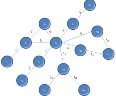
Fig. 6 Network of non-directional business relations
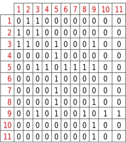
Figure 7 presents amatrixwhich shows the existence of the connections between the various actors of the network proposed in Figure 6, represented by a non-directional graph. In beingnon-directional, a matrix is symmetrical.
10 1 2 3 4 5 6 7 8 9 10 11 1 0 1 1 0 0 0 0 0 0 0 0 2 1 0 1 0 0 0 0 0 0 0 0 3 1 1 0 0 1 0 0 0 1 0 0 4 0 0 0 0 1 0 0 0 0 0 0 5 0 0 1 1 0 1 1 1 1 0 0 6 0 0 0 0 1 0 0 0 0 0 0 7 0 0 0 0 1 0 0 0 0 0 0 8 0 0 0 0 1 0 0 0 1 0 0 9 0 0 1 0 1 0 0 1 0 1 1 10 0 0 0 0 0 0 0 0 1 0 0 11 0 0 0 0 0 0 0 0 1 0 0
Fig. 7 Symmetrical matrix for the non-directional graph in Fig. 6
Each element of the matrix shows a connection, or the lack of it, between two actors and is notated “xline, column”, with the sub-indices indicating the actor of a given line and the actor of a given column. If considering the values of “i” and “j” as these indices, each element will be identified byxij or algebraically:
= 1 - when there is a connection between and
= 0 - when there is no connection
= = 0 - when the connection does not exist and in the symmetrical matrix: = .
Therefore, if the connections aredirectional, the graph is directional, and in this case the notation will be:
= 1 - when there is a connection from to
= 1 - when there is a connection from to
= 0 - when there is no connection
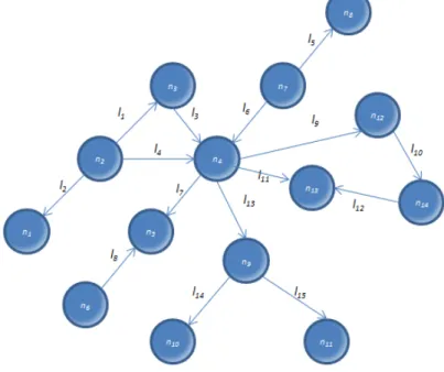
and here the matrix is rarely symmetrical. In Figure 8 is presented a directional graph where the companies have selling relationships between each other. The arrows point in the direction of the sale.
11
Figure 9 presents the corresponding sociomatrix, where can be seen the asymmetry and that the main diagonal is empty. 1 2 3 4 5 6 7 8 9 10 11 1 - 0 1 0 0 0 0 0 0 0 0 2 1 - 1 0 0 0 0 0 0 0 0 3 0 0 - 0 1 0 0 0 1 0 0 4 0 0 0 - 1 0 0 0 0 0 0 5 0 0 0 0 - 0 1 1 0 0 0 6 0 0 0 0 1 - 0 0 0 0 0 7 0 0 0 0 0 0 - 0 0 0 0 8 0 0 0 0 1 0 0 - 0 0 0 9 0 0 0 0 1 0 0 1 - 1 1 10 0 0 0 0 0 0 0 0 0 - 0 11 0 0 0 0 0 0 0 0 0 0 -
Fig. 9 Sociomatrix corresponding to the directional graph in Fig. 8
In the next section, using the basic knowledge of graphs and sociomatrices, various characteristics of the networks of business relationships, such as prestige, social role of the actors and other definitions which are useful in the practical analyses in business and social environments are being defined.
3.2
Measures in Social Networking
The use of graphs and sociomatrices is necessary in order to createmodels, or simplified representation systems of networks of relationship. However, with graphs and sociomatrices it is not possible to represent the whole of the characteristics and attributes of a network, nor all of its limits and variations. In order to make analyses therefore, the model is simplified and the analysis is based on various measures. The main measures used for social network analysis are presented in this section.
Nodal degree
In a non-directional network, it is measure the number of connections at a node and this number is called the nodal degree. The degree of a node can vary from zero, when there is no connection at this node to any other node of the network, through to the valuef – 1, when there is a connection at this node with all the other nodes on the network. The measure of the degree of a node can define its importance, for example, in a network where there are various connections, this is something of interest to the members of the network.
To obtain a graph of the degree of a given node,g(ni), count the number of lines which are connected to this node. Considering the example shown in Figure 6 and then checking the degree of each node, in decreasing order, as follows:
( ) = 6
( ) = 5
( ) = 4
( ) = ( ) = ( ) = 2
12
An important piece of data in business networks is the average number of relationships between the members of the network. This can be measured by obtaining the average degree of the network. The average degree is defined by the sum of all the degrees divided by the number of actors in the network or algebraically:
̅=∑ ( )=2
where L is the number of connections of the network and f is the total number of actors (nodes). For the network from the previous example, the value of ̅ = 2.36.
Nodal degree (directional graph)
In directional graphs, the measure of the degree is slightly different, as it is interesting to know how many connections the origin node has and how many connections it has as destination.
The number of connections this node has as destination is callednodal-in degree. For the nodal-in degree of nodeni, obtained by counting the number of arrows pointing towards it. The used notation is gi(ni).
The number of connections this node has as origin is called nodal-out degree. For the nodal-out degree of nodeni, obtained by counting the number of arrows pointing from it. The used notation isgo(ni).
These measures are very important in a network, as thenodal-out degreecan indicate the capacity of expansion of a given actor, whilst the nodal-in degree can represent their popularity. The measure of the nodal-in degree, for example, is one of the factors which determines the status of a given web site when making a search using Google. The position in the ranking of a page shown in the search results is determined by the number of sites which link to that page on the network, in other words, the nodal-in degree of the page.
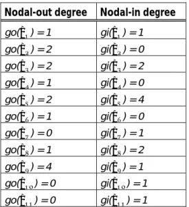
For the business network considered in Figure 8, showing the directed connections for sales from one actor to another, the next nodal-out degree and the nodal-in degree are calculated for each node:
Nodal-out degree Nodal-in degree go( ) = 1 gi( ) = 1 go( ) = 2 gi( ) = 0 go( ) = 2 gi( ) = 2 go( ) = 1 gi( ) = 0 go( ) = 2 gi( ) = 4 go( ) = 1 gi( ) = 0 go( ) = 0 gi( ) = 1 go( ) = 1 gi( ) = 2 go( ) = 4 gi( ) = 1 go( ) = 0 gi( ) = 1 go( ) = 0 gi( ) = 1
13
In the table above can be seen that for the same node the nodal-out degree and the nodal-in degree may be either equal or not. Based on the differences of in and out degrees, the theoreticians of directional graphs have created different names for the roles of the nodes (Wassermann [1994]). This is of special interest in business networks, as they define the behavior of the actor in the network of relationships.
Furthermore, depending on the number and type of connection, differenttypes of nodeare defined:
Isolated if ( ) = ( ) = 0 - neither the origin nor destination of connections
Transmitter if ( ) = 0 and ( )≥1 - not the destination of connection, but the origin
Receptor if ( ) = 0 and ( )≥1- not the origin of connection, but the destination
Carrier if ( )≥1 and ( )≥1- the origin and destination of connection
For the considered example, the company node 5 is a carrier and acts as intermediary as a seller in this network, but also concentrates most of the buying (its nodal-in degree is by far the highest). As for the non-directional graph, it is important to find the average nodal-in degree and the average nodal-out degree of the members of such a network. The average nodal-in degree, denoted by , is defined as the sum of all the nodal-in degrees divided by the number of actors of the network, that is:
=∑ ( )
wherefis the total number of actors (nodes). Similarly, the average nodal-out degree, denoted by , is defined as the sum of all the nodal-out degrees divided by the number of actors of the network, that is:
=∑ ( )
The total number of “ins" have necessarily to be equal to the total of the “outs” (the sum of all the origins should be equal to the sum of all the destinations). The next formulation is possible:
= =
whereLis the number of connections of the network. For the network in the above example, the value of = = 1,27 , which represents a directional network with low connectivity.
Density of the network. Whilst the degree of the node is important to define the number of relationships of a given actor, another important piece of data of a network is itsdensity, in other words, the measurement of the number of existent connections. Dense networks are those in which there are many connections and sparse networks are those where there are few connections. Environments where there are intense business relationships, such as between the countries of the European Union form dense networks.
The measurement of the density of a non-directional network is denoted by∆ and it is defined by the number of connectionsLof this network divided by the maximum numberlmaxof connections.
The expression for the density for the non-directional graph is: ∆ = (
−1) 2
= 2
14
If the graph has no connections, it is said to be empty and the density is equal to 0. If it has the maximum number of connections, then it is said to be full and the density is equal to 1. Figure 10 exemplifies the empty, the full and the intermediate graph, for a network with four nodes.
Fig. 10 Density of different non-directional graphs
For a directional network, the measurement of the density is denoted by and is defined by the number ofLconnections (arrows) of this network divided by the maximum numberlmax.dir. The expression for the density for the directional graph is:
∆ =
( −1)
Walk, trail and path
In a network, there may be some type of relationship between two nodes, even if there is no direct connection between them, but through a third node, for example, with which both nodes have a connection. An example can be: if Mary is a friend of Jon and Jon is a friend of Joyce, it is possible that Mary and Joyce get to know each other and also become friends.
Fig. 11 Walks, Trails and Paths in a network
The various connections function as a kind of network of channels, and as the network becomes more complex, the complexity of paths through these various channels becomes greater. In a graph representing a network, from one actor to any other one it is possible to trace paths passing through various connections. For these paths, there are used the following definitions:
15 Walk– sequence of nodes and connections, starting out from one node and ending at another node, passing through the connections which join the various nodes of the route made. Nodes and connections can be repeated or not, with the length of the walk being defined by the number of connection lines travelled. In the example in Figure 11, the sequence {n6, l8, n5, l7, n4, l6, n7, l6, n4} is one walk in which the nodesn4andl6are repeated, and the total length of the walk equal to 4.
Trail– a trail is a special type of walk in which all the connection lines are distinct, but the nodes can be repeated. In Figure 11, an example of a trail is the sequence {n5, l7, n4, l3, n3, l1, n2,l4, n4}, in which the noden4is repeated. In this trail the total length is equal to 4.
Path– the path is another special case of walk in which all of the nodes and connection lines are distinct, and there can be no repetitions. One example of path in Figure 11 is the sequence {n6, l8, n5, l7, n4, l6, n7}, whose length is equal to 3.
Note: In a network of relationships these concepts are fundamental for calculating the distances between actors, and then to set up, between companies, for example, possible negotiations based on mutual relationships.
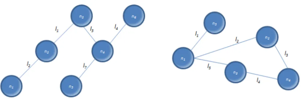
If the graph isdirectional, as in the example in Figure 12, these paths can be interpreted slightly differently. The idea of direction has to be attributed and if designating the connections as “arrows”, the next measures can be considered:
Directed walk– sequence of nodes and arrows, leaving from a node and ending at a node,passing along the arrows always in the same direction, which link the various nodes of the path travelled. Nodes and arrows may be repeated or not, and the length of the directed walk is defined by the number of arrows. In the example in Figure 12, the sequence {n7, l6, n4, l4, n2, l1, n3, l3, n4, l4, n2, l2, n1} is the directed walk in which the nodesn4andn2 and the arrowl4 are repeated, and the total length of the walk is equal to 6.
Fig. 12 Directed walks, Trails and Paths in a directional network
Directed Trail– similarly, the directed trail is a special type of walk in which all the arrows of the connection are distinct and always in the same direction, but the nodes may be repeated. For the proposed example, the sequence {n7, l6, n4, l4, n2, l1, n3, l3, n4, l13, n9} is a directed trail in which the node n4 is repeated, and the total length is equal to 5.
16 Directed Path– in this case, all the nodes and connection arrows are distinct, and thearrows are
always in the same direction, without repetitions. An example of directed path in the previous figure,
Fig. 12, is the sequence {n2, l1, n3, l3, n4, l13, n9, l14, n10whose length is equal to 4.
Note: If for the previous three cases some of the arrows on the path travelled had the opposite direction, then the denominations would besemi-walk, semi-trail and semi-path respectively.
Closed walk
A sequence is called aclosed walkwhen the walk begins and ends on the same node. There is no problem if some lines and nodes are repeated. An example of closed walk in the graph in Figure 11 is the sequence {n5, l7, n4, l3, n3, l1, n2,l4, n4, l7, n5} in which nodesn4andn5are repeated, and the walk begins and ends at noden5.
Cycle
A sequence is called acyclewhen there are at least three nodes and the start-node is the same as the end-one and the connection lines are not repeated. An example of a cycle in the graph in Figure 11 is the sequence {n4, l3, n3, l1, n2,l4, n4}.The concept of cycle is the same fordirectional graphs, provided that all the arrows point in the same direction on the path travelled. In Figure 12 a cycle is defined by the sequence {n2, l1, n3, l3, n4, l4, n2}.
Semi-cycle
In adirectionalgraph asemi-cyclesequence is a cycle in which at least one of the arrows points in the opposite direction to the others. An example of semi-cycle in the graph in Figure 12 is the sequence {n4, l9, n12, l10, n14, l12, n13, l11, n4}.
Searchability and directional connectivity
In a network, if there is a path between two nodes, this means that these two nodes can establish some type of relationship along this path formed by the path, that is, a node can find the other node along the path. This possibility of relationship is calledsearchability.
17
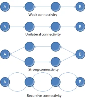
In adirectionalgraph, searchability can be established at different levels, depending on the direction of the arrows along the path. For a node to be able to find the other node in a directional network, there are four types of connectivity, as shown in the example of types of paths between nodesAandBin Figure 13. These are the four types of connectivity:
The nodes A and B have weak connectivity between then when there is a semi-path between them (at least
one arrow in the opposite direction)
The nodes A and B have unilateral connectivity between then when there is a directional path from A to B
or from B to A between them (all arrows point in the same direction)
The nodes A and B have strong connectivity between then when there is a directional path from A to B and
another directional path from B to A (passing through different nodes and connections)
The nodes A and B have recursive connectivity between then when there is a directional path from A to B
and from B to A passing through the same nodes and connections.
Every directional graph comes within one of these types of connectivity. Their interpretation is:
The directional graph has weak connectivity if all the pairs of nodes have weak connectivity
The directional graph has unilateral connectivity if all the pairs of nodes are connected unilaterally
The directional graph has strong connectivity if all the pairs of nodes have strong connectivity
The directional graph has recursive connectivity if all the pairs of nodes have recursive connectivity
Note: These ideas are important for the analysis ofcohesion between the members of a given network. If there is weak connectivity betweenAandBin a business network of sales, the possibility of Aselling toBis less than if the connectivity were strong.
Connected and disconnected network
A network is consideredconnectedif there is a path between any pair of nodes of this network, that is, if any actor in the network can establish a relationship with any other, even if it means going through various intermediate connections and actors. If this is not possible, the network isdisconnected.
This concept is very important because it allows one to see if a business relationship can be established using a given network, or because it enables one to see which connections could be taken out to “disconnect” the network and, for example, the connections of a terrorist network could be destroyed, if that were so desired.
18 Geodesic
The shortest path between two nodes is calledgeodesic, and the length of this path, in number of intermediate connections, is calledgeodesic distance. This minimum distance is very interesting because it allows the analyst to see how many connections and how many nodes are intermediaries in a relationship between two actors of a network. The geodesic distance between any two nodesniandnj, is notedd(ni, nj).
If there is no geodesic for any two nodes, that is, if there is no possibility of any path between them, their distance is considered infinite and the network will be disconnected.
For a directional network, the geodesic is considered as the shortest directed path between two nodes. Considering that in a directed path all the arrows have to be in the same direction, the geodesicfromnitonjwill not always be the same geodesic fromnjtoni. See an example of this type in figure 2.15. The sequence which defines the geodesic fromn1ton3is {n1, l2, n2, l3, n4, l4, n3}, with the geodesic distanced(n1, n3)=3.Whereas for the geodesic fromn3ton1, the sequence is {n3, l5, n1}, with the geodesic distanced(n3, n1)=1.
Fig. 15 Examples of geodesic in an undirected and a directed network
Diameter
Having established the geodesic distances of a connected network, the greatest distance will determine thediameterof this network. In the example in Figure 15, the diameter of the undirected network is equal to “4”, as the greatest distance is established by the geodesics:
d( , ) = 4 and d( , ) = 4
The diameter for a directional network follows the same principle, considering the greatest directional geodesic distance of any pair of nodes of the network. For the directional network in Figure 15, the diameter is equal to 4, defined by the geodesic distance fromn5ton3:
d( , ) = 4
“Cut node” - Cut-point
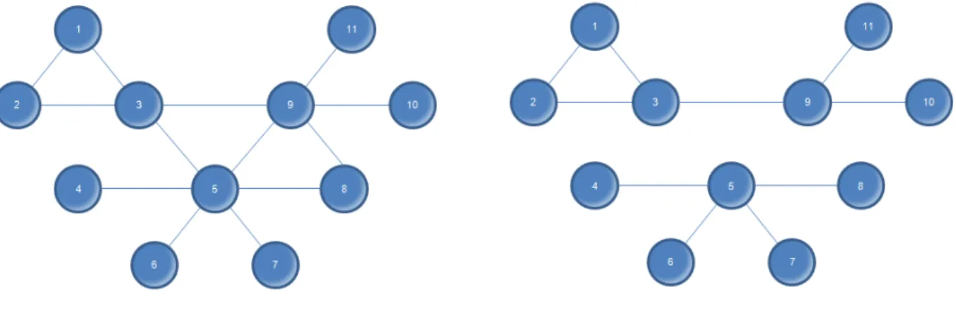
Acut-pointis a node which if it was taken out, would make the network disconnected, dividing it into different “components”. There are very important cut-points, because they can divide the network into different and non-communicating parts, which weakens the network considerably. The taking-out of a node implies the disappearance of all its connections. As example, if taking-out noden4from the network in Figure 12.10, the result would be as shown below, in Figure 16.
19 Fig. 16 Disconnected network by taking out the cut-point
The network became fragmented (disconnected) and five sub-graphs or components resulted from the original graph. No other cut-point from this network can cause so much damage. Most of the nodes in this network are not cut-points (as they do not separate the network into different components). In the considered example, other cut-points aren2, n5, n7 andn9. Obviously taking- out another node affects the network quite differently than the previous one. This type of study in terrorist or organized crime networks has been done to find out which are the most important cut-points that could weaken the organization.
Bridge
The idea ofbridgeis similar to that of cut-point, but it refers to the connection which if it was taken out from the network, would make the network disconnected, dividing it into different “components”. All the nodes remain in the network, and just the connection which represents the bridge is taken out, resulting in a disconnected network. In the example in Figure 17, linel3is the bridge. If it is taken out, the network becomes two components and nodesn1, n2 andn3 are not paths to nodesn4, n5 andn6.In a business environment, the connection which acts as a bridge could be a contract or an agreement. The termination of such an agreement could cause isolation, for example, of two groups in the business network who would no longer relate to each other.
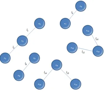
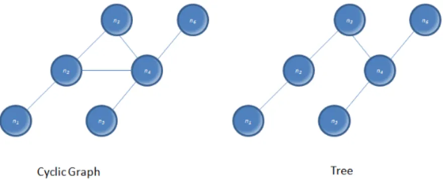
20 Cyclic graph and tree
Every graph which contains cycles can be called acyclic graph. However, if a network represented by this graph has no cycle, it will be called atree. The tree is a special network because it is weakly connected and each connection is a bridge. Any connection, if it is a taken-out, will cause a disconnection of the network. For this reason, networks in the form of a tree are not good for the business environment and any problem with an actor or a connection will affect the development capacity of the network.
Fig. 18 Example of cyclic graph and tree type network
Bipartite graph
A graph can be consideredbipartite if the relationships get established between two sets of actors, but with no connections between the actors within the same set. This is a special case of networks, and a practical example is in the formation of the network of distance learning relationships.
Suppose that one set of actors consisting of teacher-tutors and the students are using the tutoring tool. The teachers will be in one of the sets and the students in the other, and the connections are the various questions and answers. Not all the students establish communication with all the teachers, and not all the teachers answer all the students. If there are connections from all the actors in one set to all the actors in the other, it will be a fully bipartite graph. The concept is presented also graphically below, in Figure 19.
21 Graphs with sign and with value
For each relationship established by a connection in a graph, two further pieces of additional information can be included: asignand avalue. The inclusion of a positive or negative sign for a connection can show us that a relationship is good or bad. An example of this type of network is a graph showing the relationships of affinity between students in a classroom. Usually (+) indicates that there is friendship and (–) indicates enmity.
The inclusion of value can add a number to a connection. An is indicating on the graph the business relationship between companies, the value of the connection representing the amount in millions of dollars in a sale transaction.
Centrality and prestige
Two important concepts in a network are the ideas ofcentralityandprestigeof an actor. There are various definitions and forms of calculating centrality.
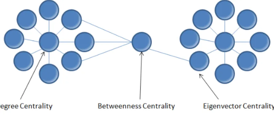
For a given actorni, the centrality is denoted asC(ni)and the measure will be given by the degree of the node, that is, by the number of connections of this node in the network. Centrality can be also considered the measure that gives the indication of power and influence of the individual nodes of the network based on how well they are connected. The fundamental measures of centrality are: Betweenness, Closeness, and Degree.
Betweenness measures the number of subjects whom an individual is connecting indirectly, through their direct links.
Closeness indicates how near is a subject to all other individuals in a network, directly or indirectly. Closeness centrality is the inverse measure of the sum of the shortest distances between each individual and everyone else in the network.
Fig. 20 Example of centrality
Centralization is the difference between the numbers of links of each node in the network divided by maximum possible sum of differences. A centralized network will have many of the links dispersed around a certain node(s) while a decentralized will have nodes with comparable number of links. The concept of prestige of an individualniis related to the concept of directional networks. The centrality of an individual ni, considering the arrows directed towards them (i.e. their nodal-in degree) defines his prestige,P(ni),in the network.
22 Other metrics in Social Networking
Clustering coefficient is the measure representing the probability of a future link between two unconnected neighbors of a considered node.
Cohesion represents the degree in which nodes are connected directly among each other by cohesive bonds.
Radiality represents thedegree with which the network of a certain individual reaches out into the global network providing content and inducing influence.
Reach represents the degree in which any node of a network can reach the other nodes.
Structural cohesion measures the minimum number of nodes that would disconnect the network or the group if removed.
Structural equivalence represents the degree in which nodes share a common set of links connecting them to other nodes in the network
Analysis of network data can be done on different levels: node level (i.e. centrality, prestige, node roles such as bridges, isolates etc.); dyadic level (referring structural distance and reachability, notions of equivalence, reciprocity etc.); triadic level (referring aspects of balance, transitivity etc.); subset level (i.e. cliques, (cohesive) subgroups, network components etc.); global network level (referring aspects of connectedness, diameter, centralization, density etc.).
23
4. Behaviour and Dynamics in Social Networks
Connectedness in social networks implies two aspects: the structural connectivity (which network entity is linked to which network entity) and the behavioral connectivity (individual actions affect all other entities in the network). This is why, aside the understanding of the network structure, it is important to understand the network interaction and behavioral dynamics.
Both the structural and behavioral levels present high complexity. Considering the behavioral aspect, if the entities in the network are actively involved in the considered community, these will appreciate their influence and will consider it with their new actions. A fundamental consideration must be the fact that community behavior is continuously changing. In any social network, the behavioral shifting and evolution is caused by both internal and external factors. The network behavioral models are based on the network entities strategic reasoning and behavior, considered in social context and not in isolation. Behavioral impact in a network should be considered both from the network and the individual point of view: as prior mentioned, an individual action has impact on the behavior or / and structure of the entire network and vice versa, the network behavior and evolution has impact on the individual behavior.
Considering the first type of dependency, the network behavior and evolution are influenced either by individual characteristics, structural positioning, connectivity activity etc. This type of dependencies is described as the selection processes. An exemplification of such dependency is the homophily process: the creation of network relationships based on entity similarity.
On the other hand, networks can affect the individual characteristics and their behavioral development. Such dependency is described as influence processes. An exemplification is the assimilation process: similarity of individuals that are highly socially connected.
Influence and selection processes are strongly interdependent. Separating these is difficult as the network data is inherently interdependent.
A future connection of two individuals might depend on their relationship with third-party individuals. Not many statistical models can detect such network dependencies. An established approach for the analysis of longitudinal network data is the Stochastic actor-based modeling, Snijders [1996]. Extensions of this approach can help the simultaneous analysis of selection and influence processes, based on the interdependence between these processes - Snijders, Van de Bunt and Steglich [2010]; Steglich, Snijders and Pearson [2010].
Large real-world networks are highly dynamic and exhibit a range of interesting properties and patterns. One of the recurring themes in the line of behavioral and dynamics research is to design models that predict and reproduce the emergence of such network structures. Research then seeks to develop models that will accurately predict the global structure of the network. The following sections introduce the concept of structural balance in Social Networks and present specific models for the Link Prediction problem.
Chapter 5 presents a behavioral case study of structural influence based on the centrality and power graph theory approach. The technology presented is UCINET, a dedicated tool for social networking analysis, the investigation being conducted on the UCINET dataset, Bernard & Killworth Fraternity (BFRAT).
Chapter 6 presents a second study, with focus on the accuracy performance of link prediction models. A set of three models are used: Support Vector Machine (SVM), K-Nearest Neighbor and Naïve Bayes and the link prediction investigation is done on the DBLP co-authorship dataset using the following set of features: sum of papers, weighted sum of neighbors, weighted sum of secondary neighbors and weighted shortest distance.
24
4.1
Structural Balance of Social Networks
Social relationships have a profound impact on human development, in all life stages. Such relationships are of positive nature (i.e. friendship, collaboration, trust, support etc.) or of negative nature (i.e. oppression, dislike, harassment, intimidation etc.). A social network captures all such types of relations defined between a finite set of members. Individual characteristics and shared relationships change in time and continuously impact the entire community (social network).
Clearly, the tension executed between every two network entities, be it positive or negative is a fundamental aspect in social networking. The framework of this type of analysis is the structural balance, which aims to extract and store the relationship information in a clear and structured way. The structural balance concept is based on social psychology theories being helped by graphical and mathematical representations. The structural balance theory is based in fact on pure mathematical analysis.
The structural balance theory is based on identifying the nature of relationship between two individuals by initially isolating them. If these individuals share some level of friendship, support or collaboration, their link is marked positive: “+”, else the link is marked negative: “-“. The theory looks at subgroups of three individuals sharing a particular configuration of positive and negative values. In fact, there are possible four distinctive configuration cases between three individuals A, B, C. These are presented in Figure 21 below.
Fig. 21 Structural balance for sets of three nodes
In such reduced systems, clear conclusion of structural balance can be drawn:
Case 1: A, B, C are mutual friends. This is a natural situation of three persons that are mutually friends. There are no instability sources in such system, therefore the system is balanced.
Case 2: A, B are friends and C is a mutual enemy. This is also a natural situation between three individuals, two of the three are in a relationship of friendship and both dislike the third individual. As the system has clear friendship and enemy bindings and therefore no instability sources, this system is balanced.
25 Case 3: A is friend with B and C, but B and C are enemies. In such system there is present, in some degree, a psychological stress or instability into the formed relationships: one individual is in a friendship relation with two other individuals that dislike each other. The instability source comes from the fact that individual A might try changing the negative relation between B and C in positive one or might take side and become enemies with one of the individuals B or C. Based on this instability reasoning, this system in unbalanced.
Case 4:A, B, C are mutual enemies. In this type of system there are also present instability aspects. The reasoning is based on the fact that two individuals might start collaborating against the third individual in the system. In this case a negative link might transform in a positive one. This is why this system too is considered unbalanced.
In conclusion, the structural balance of a sub-system of three individuals connected by three links is achieved if: either all three links are positive or else, only exactly one of the links is positive. This consideration is known as the structural balanced property and is at the basis of the global structural balance of the network.
The global structural balance of the network is expressed as the problem of eliminating the unbalanced triangles. This expression is not convenient due to the involved computation, but it represents the basic start point in the concept of structural balance of social networks. A more mature formulation of structural balance in a social network is the Balance Theorem, given by Frank Harary [1953]:
“If a labeled complete graph is balanced, then either all pairs of nodes are friends, or else the nodes can be divided into two groups, X and Y, such that every pair of nodes in X like each other, every pair of nodes in Y like each other, and everyone in X is the enemy of everyone in Y.”
Today structural balance is highly relevant in the on-line social media where individual opinion is intensively expressed, often in a context of influence. Another example is the international relations, representing the relationship between various countries.
Understanding the mechanism of positive and negative relationships helps the studies of behavior, structure and influence in the social field. These are important aspects in managing social or business contexts. Research is only starting exploring these fundamental questions, aiming to understand how, out of large scale datasets, balance and related theories can bring out knowledge.
26
4.2
Link Prediction Models
Social networks present high dynamics and a continuous transformation by adding new nodes and edges. This behavior causes changes in the nature of the social interaction and the structure of the network. For various domains it would be a great benefit to be able to understand and therefore control the mechanism of evolution of social networks.
Apart from influence, another fundamental topic in the evolution of social networks is the link prediction problem. This subject has captured the attention of various scientists, especially in the artificial intelligence sector and data mining.
Many studies refer business and professional collaborations generated by informal social interactions in such networks. Other studies focus on the impact of the social hierarchy in the professional network or inferring missing links. It is interesting to notice that most of these studies conclude that effective and concrete link prediction methods can be used to analyze social networks so to predict future interactions that might help organizations, businesses or investigations.
The social network analysis proved a significant role in domains as security, terrorism, biology, sales and many others. In some of the domains, such as security and terrorism, the type of prediction is of a link between groups of individuals that collaborate, but not by an obvious connection. In domains similar to sales, a typical type of link predictions regards the potential collaboration based on observations of business and informal interests and actions.
Today, due to the large amount of available social networking data, studies and simulation of different nature are possible. These contribute significantly to understanding the properties and the behavior of social networks.
4.2.1 Mathematical framework
Consider a social network =( , ), where V is the set of network nodes and E is the set of edges between the network nodes, the problem of link prediction is the task to predict how likely a new link
∉ will exist between a pair of existing nodes in the network ( , ).
Often the time dimension is added to the link prediction problem so to measure the growth of the network. In this case the discussed problem should be seen as the task of accurate prediction of the edges that will be added to the network between two deterministic points in time.
The link prediction problem addresses four main aspects: link existence, link type, link weight and link cardinality. Many link prediction studies concentrate on the problem of link existence - whether a new link between two nodes in a given social network will exist in the future or not. The link existence problem is extended by the other two problems of link prediction: link weight – the links between different network nodes are given different weights and link cardinality – two nodes of a given social network are connected to more than one link. The fourth problem, the link type is a more particular problem - it refers to possible different roles of the one relationship between the same two nodes of the given social network.
The link prediction problem can be treated with techniques of various natures: statistics, probability, graph theory, machine learning etc. Depending though on the approach of analysis, the techniques can be classified in three groups:
Models based on node similarity – regards the similarity measurement between two nodes
Models based on topological patterns - local or global patterns that could define the network
27 4.2.2 Models based on node similarity
The models based on node similarity propose measurements of similarity for pairs of network nodes. In this context, the task of link prediction is the consideration of new edges between network nodes presenting a considerable similarity, usually measured against a threshold. In general, the measurement of similarity is either (pre)defined or learned (using machine learning techniques), depending on the studied domain or the type of network.
According to Lin [1998] the similarity between two network nodes ( ; ) can be defined by the percentage of the common information in the total set of properties characterizing the two nodes. The measurement is applicable in case of a probabilistic model for the studied case:
( ; ) = ( ( ; ) ) ( ( ; ) ) where , are the sets of properties characterizing the two nodes ; .
Another similarity distance measurement was given by Bennett and Li [2004] and refers to the Kolmogorov complexity measurement between the set of properties of the two nodes ( ; ). The Kolmogorov complexity measurement of a binary string ˅ is defined as the length of the shortest program for an Universal Turing Machine (UTM) to correctly reproduce the considered string, ˅. Consider ˅,˅ the binary strings corresponding to the set of properties of the two nodes, for a given UTM, the Kolmogorov complexity measurement (˅|˅) is the length of the shortest program for the UTM to output ˅ when given ˅ as input. In this context, the similarity measurement is formulated as:
(˅ ;˅ ) = { (˅ |˅ ), (˅ |˅ ) } { (˅ ), (˅ ) }
The disadvantage of such predefined similarity measurements is that they do not consider the network context. For this reason, the adaptive similarity functions are frequently learned using supervised learning techniques. Some of the most representative techniques are: Binary classifiers, Kernel methods and Statistical Relational Learning (SRL).
Binary classifiers are proposing training a binary classifier to determine the similarity between two network nodes, based on their content information. A mapping feature function is used to extract the content features of the two network nodes in a single vector ( ; ). Considering a simple linear regression, the objective of the function is learning a set of parameters that can indicate best similarity. For a candidate node pair, the link prediction problem is reduced to:
( ; ) = ,
′ ( ; ) > 0
, ′ ( ; ) < 0
Within the set of pairs not selected as candidates (negative examples), it is possible and should be considered that new links might exist. Another conclusion is that in networks with few or sparse links, the number of candidates and non-candidates pairs is considerably unbalanced.
The binary classifiers are best applicable when nodes of a certain class have many features in common, else finding pairs is very difficult and the consequence is a high recall.
28 Kernel matrices methods are proposing an alternative to the binary classifiers that suit also the case when the set of common features between nodes of the same class is reduced. One approach is capturing the content information of the network nodes in Cartesian products for pairs of features < ; >:
,
= ( , , … , , , , … , , , … , )
The problem with this approach is that the dimension of the feature set is . Clearly, the involved computation is not practical in the case of networks with a large set of node-features. Also, conducting learning in a high dimensional feature-space is challenging and may lead to over-fitting.
A better solution is the approach of Support Vector Machine (SVM) learning algorithms, suggesting pairing nodes as inner products < ; > and not considering the nodes individually. In this way, by using kernel functions ( ; ) for the defined inner products, the challenge of classification in higher dimensional feature-space can be solved. Oyama and Manning [2004] suggested the next kernel, for any instance of node-pairs in the original feature-space:
( , ) = , , , =< , >< , >
when ( ) = , and ( ) = , are instances of feature-pairs of the considered nodes. The proposed kernel is actually a tensor product between two linear kernels representing the inner products.
The link prediction problem considers the space of node-pairs as input space of nodes and the similarity between such pairs is defined by the explicit form of the proposed kernel. A high value of the kernel indicates high node-similarity. This approach has a wide applicability, especially in prediction of rating or collaborations. One specific domain of collaboration is the scientific co-authorship, and link prediction in such a community represents the subject of the second study presented in the paper.
Statistical Relational Learning (SRL) incorporates a variety of approaches and techniques. The nature of these methods can be statistical, probabilistic, logic-based algorithms etc. An established approach suggested for link prediction was established by Popescul [2003] and suggests using aggregation of relational features for measuring similarity. Various classification algorithms have been proposed and studied, many known from other disciplines such as data mining and machine learning. A particular approach is translating the link prediction problem in an optimization problem by mapping the network nodes to Euclidean spaces.
29 4.2.3 Models based on topological patterns
This approach is focused on identifying global or local topological patterns in the entire network or partial network. For fundamental concept in this approach is scoring the weight of the link between the nodes of a pair ( ; ) , in rapport to the determined topological pattern(s).
Depending on the leading element in determining the topological patterns, there can be distinguished three types of topological patterns approaches: Node based, Path based or Graph based.
Node based approaches take into consideration the neighborhood information of a node, for example the set of first neighbors that a node has. One consideration in this area is that two network nodes would more probably establish a link if they have a large number of common neighbors.
In the proposed link prediction study in the co-authorship world, due to the nature of the domain, such information is relevant and important. Scientists and researchers tend to set new collaboration with colleagues in the same area, based on the recommendations received from their collaboration partners, the first neighbors. In other words there is a high probability that a scientist will collaborate with his second neighbors. This is one topological feature considered in the algorithm comparison. A number of measurements of this nature have been already formulated and standardized. These intend to define a scoring function for a potential link between two nodes ; , most often based on structural considerations such as the number of direct neighbors a node has, noted ( ) and respectively . The most common node-based scoring functions are:
Common neighbors method – proposes a scoring function of the link between two nodes ( ; ) based on the number of common neighbors these nodes share:
( ; ) = | ( )∩ ( )|
Jaccard coefficient – proposes a scoring function of the link between two nodes ( ; ) based on the ratio between their common neighbors and the total number of their neighbors:
( ; ) =| ( )∩ ( )| | ( )∪ ( )|
Adamic/Adar coefficient – proposes a scoring function of the link between two nodes ( ; ) based on the number of their common neighbors, weighting more those neighbors
∈ ( )∩ ( ) that the two nodes share least with other nodes in the network:
( ; ) = 1
| ( )| ∈ ( )∩ ( )
Preferential attachment method – proposes a scoring function of the link between two nodes based on the premise that node will receive a connection from node two with a probability proportional to the number of neighbors of , | ( )|. And vice versa:
30 Path based approaches take in consideration the path connectivity information between two network nodes. The main idea of this type of approaches is that the more indirect paths are connecting two nodes the higher the possibility that a link will connect them directly. Many studies contributed to the theory of shortest-path distance based on analysis of the entire set of indirect links connecting two network nodes.
As in the case of the node similarity approach, a number of measures based on the path similarity have been already established. The main ones are:
Katz measure - proposes a scoring function of the link between two nodes based on the sum of the total number of paths weighted according their length. If the ℎ ,
( )
denotes all paths of length l between two network nodes ( ; ) then the formulation of the Katz measure is:
( ; ) = | paths ; ( )
|
∞
where > 0 is a parameter of the predictor.
,
Hitting time measure – proposes a scoring function of the link between two nodes based on the required steps to reach