promoting access to White Rose research papers
White Rose Research Online
[email protected]
Universities of Leeds, Sheffield and York
http://eprints.whiterose.ac.uk/
This is an author produced version of a paper published in Transportation.
White Rose Research Online URL for this paper:
http://eprints.whiterose.ac.uk/77197/
Paper:
Hess, S and Hensher, D (2013)
Making use of respondent reported processing
information to understand attribute importance: a latent variable scaling approach.
Transportation, 40 (2). 397 - 412.
Making use of respondent reported processing information to
understand attribute importance: a latent variable scaling approach
Stephane Hess∗ David A. Hensher†
May 23, 2012
Abstract
In recent years we have seen an explosion of research seeking to understand the role that rules and heuristics might play in improving the predictive capability of discrete choice models, as well as delivering willingness to pay estimates for specic attributes that may (and often do) dier signicantly from esti-mates based on a model specication that assumes all attributes are relevant. This paper adds to that literature in one important way - it explicitly recognises the endogeneity issues raised by typical attribute non-attendance treatments and conditions attribute parameters on underlying unobserved attribute im-portance ratings. We develop a hybrid model system involving attribute processing and outcome choice models in which latent variables are introduced as explanatory variables in both parts of the model, explaining the answers to attribute processing questions and explaining heterogeneity in marginal sensi-tivities in the choice model. The resulting empirical model explains how lower latent attribute importance leads to a higher probability of indicating that an attribute was ignored or that it was ranked as less important, as well as increasing the probability of a reduced value for the associated marginal utility coecient in the choice model. The model does so by treating the answers to information processing questions as dependent rather than explanatory variables, hence avoiding potential risk of endogeneity bias and measurement error.
Keywords: information processing; attribute ignoring; non-attendance; attribute importance; attribute relevance; stated choice
1 Introduction
There is a growing recognition that when faced with a typical stated choice (SC) scenario where each alternative is described by a number of attributes, dierent respondents will process the information in dierent ways. The main emphasis has been on the notion that individual respondents may make their decisions only on the basis of a subset of the attributes describing the alternatives, a phenomenon variably described as attribute ignoring or attribute non-attendance. The origins of this research stream
∗Institute for Transport Studies, University of Leeds, Leeds LS2 9JT, [email protected], Tel: +44 (0)113 34 36611,
Fax: +44 (0)113 343 5334
†Institute of Transport and Logistics Studies, The Business School, The University of Sydney, NSW 2006 Australia,
are in the work ofHensher et al.(2005), who posed the very simple question what implications on WTP would there be if we recognised that some attributes are deemed not relevant by a respondent in the way that they processed the alternatives on oer?". This paper began the interest in discrete choice analysis in recognising that attribute non-attendance may be a very real heuristic impacting on the way that individuals process information in real markets for many reasons, be it cognitive burden and/or simply a recognition that specic attributes (and their levels) are not of sucient relevance to be sources of inuence on choosing. Another possible reason is the lack of sucient incentives in the scenarios presented to respondents in the context of hypothetical surveys - i.e., a given individual's sensitivity to a specic attribute may be so low that with the combinations presented, it cannot possibly have an inuence on the choice.
Since 2005 we have seen an explosion of research papers, especially in transportation and environmen-tal science, seeking to understand the role that rules and heuristics might play in improving the predictive capability of choice models, as well as delivering WTP estimates for specic attributes that may (and often do) dier signicantly from estimates based on a model specication that assumes all attributes are relevant. While the origins of this stream of work can be found in transport, applications now range across numerous dierent elds (see e.g.Cameron and DeShazo,2011;Alemu et al.,2011;Hoyos et al.,
2011;Balcombe et al.,2011;Hole,2011b; Scarpa et al., 2011; Carlsson et al.,2010). Hensher (2010) summarises the main contributions up to 2009.
Within the contributions to date, some focus on the role of supplementary questions on how attributes are processed (e.gHensher,2006;Puckett and Hensher,2008) while other studies focus on how attribute processing can be inferred from the data through advanced model specications (e.g.Scarpa et al.,2009;
Hess and Hensher, 2010). Although there has been a particular focus on attribute non-attendance, the range of potential attribute processing strategies within compensatory and semi-compensatory attribute choice settings are numerous, and will direct the research agenda for many years. There is a growing view that the consideration of alternative behavioural paradigms on how respondents process attributes in a choice making context may well add greater value to our understanding of decision making than the advances made in sophisticated econometric choice models; however the combination of both may well deliver the best outcome. It is in this area that the contribution made in the present paper falls.
As already alluded to above, there are two separate strands of research in the eld. In the rst, analysts condition their models on respondent stated attribute processing information, while, in the second, analysts attempt to infer processing strategies from the data, generally by making use of probabilistic methods. The motivation for steering clear of respondent reported processing strategies in the latter body of work has two components. Firstly, given the likely correlation between respondent reported processing strategies and other unobserved components, it should be recognised that conditioning our model specication on such information may lead to endogeneity issues which could in turn lead to biased parameter estimates. Secondly, it has been shown by a number of authors (e.g. Hess and Rose,
2007;Hess and Hensher, 2010) that there is no one-to-one correspondence between stated processing strategies and actual (i.e. revealed) processing strategies. Indeed, the results for example in Hess and Hensher (2010) show that respondents who indicate that they ignored a given attribute often still show a non-zero sensitivity to that attribute, albeit one that is (potentially substantially) lower than that for the remainder of the population. A possible interpretation of these results is thus that respondents who indicate that they did not attend to a given attribute simply assigned it lower importance, and that the probability of indicating that they ignored a given attribute increases as the perceived importance of that attribute is reduced.
valuable information, but that such data should not be used deterministically as an error free measure of attribute non-attendance, given the risk of endogeneity bias as well as the possible dierences with actual processing strategies. Rather, one should recognise that such data are simply a function of respondent-specic perceived attribute importance. The present paper puts forward a modelling framework in which this information is treated in precisely this manner. In particular, we formulate a structure that jointly models the response to the stated choice component and the response to the attribute processing questions. Crucially, the latter are treated as dependent variables rather than as explanatory variables as has been the case in work thus far. The link between the two model components is made by a number of latent variables, relating to the unobserved respondent-specic importance measure for each attribute. These latent variables are used as explanatory variables in both parts of the model, explaining the answers to attribute processing questions and explaining heterogeneity in marginal sensitivities in the choice model.
The approach used here has similar aims to the work ofHensher (2008) andHole(2011a) in that it aims to jointly model process and outcome, but we do this via the use of latent variables. As such, the model ts into a growing body of research on hybrid choice models (cf.Ben-Akiva et al., 2002;Bolduc et al., 2005). While a typical choice model explains only the choices observed in the data, a hybrid model contains additional sets of explanatory variables, for example answers to attitudinal questions. At the heart of such hybrid models are one or more latent constructs that contribute both to the utility function in the choice model component as well as the measurement models used to explain the remaining dependent variables, e.g. answers to attitudinal questions. In the most common application of hybrid models, the latent variables relate to underlying unobserved attitudes, while, in our case, they relate to the underlying importance of the dierent attributes.
Our results show that the resulting model is able to explain how lower latent attribute importance leads to a higher probability of indicating that an attribute was ignored or that it was ranked as less important, as well as increasing the probability of a reduced value for the associated marginal utility coecient in the choice model. Crucially, the model treats the answers to information processing questions as dependent rather than explanatory variables, that way preventing risks of endogeneity bias as well as avoiding the use of answers to information processing questions as error free explanatory variables, which could have exposed us to measurement error. We compare the results from our model to those from a simple MMNL model and a MMNL model conditioning on respondent reported attribute non-attendance. We nd that the hybrid model produces the most intuitively correct willingness-to-pay patterns, where the model making use of non-attendance information as explanatory variables produces the least realistic results, reinforcing earlier concerns.
The remainder of this paper is organised as follows. We rst outline the model structure in Section
2. This is followed by the presentation of the empirical analysis in Section 3. Finally, we present the conclusions of the research.
2 Methodology
In a traditional random utility model, we have that the utility of alternativeifor respondentn in choice scenariot is given by:
where Vint is the deterministic component of utility and εint is the random component of utility. With J alternatives (j= 1, . . . , J), the probability of alternativeibeing chosen is given by:
Pint(β) =P(Vint+εint> Vjnt+εjnt, ∀j6=i) (2)
The deterministic component of the utility is given by a function of observed attributesxand estimated parametersβ, i.e. Vint(β) =f(xint, β), where typically, a linear in parameters specication is adopted. In the widely used Mixed Multinomial Logit (MMNL) model, we accommodate random (i.e. unex-plained) variations across respondents inβ, and with a type I extreme value distribution for the remaining error term ε, we now have:
Pint(Ω) = Z
β
eVint(β)
PJ
j=1eVjnt(β)
h(β|Ω) dβ = Z
β
Pint(β)h(β |Ω) dβ (3)
where β ∼h(β |Ω), withΩ giving a vector of parameters to be estimated, for example the mean and standard deviation. This model collapses back to a standard Multinomial Logit (MNL) structure (i.e. Pint(β)) if no random heterogeneity is retrieved. We will typically also work with repeated choice data, and under an assumption of intra-respondent homogeneity, the likelihood of the actual observed sequence of choices for respondentn is then given by:
Ln(Ω) = Z
β "T
Y
t=1
Pi∗nt(β)
#
h(β|Ω) dβ, (4)
where i∗ntrefers to the alternative chosen by respondent nin choice situation t.
Let us now assume that as part of the survey, the analyst collects not just information on the choices made by the respondent, i.e. i∗nt, ∀n, t, but in addition captures answers to questions relating to information processing strategies. In particular, with K dierent attributes (and hence K dierent associatedβ parameters), it has become coming practice to collect data on respondent reported attribute non-attendance (or ignoring) for each of these attributes, say NAnk, k= 1, . . . , K, where NAnk is equal to1 if respondentnstates that he/she did not attend to attributexk in making his/her choices. Let us further dene Ank = 1−NAnk∀k.
In the most simplistic modelling approach, these additional measures would then be used as explana-tory variables in our model specication, where βk would be replaced by Ankβk. This means that the parameter βk is set to zero for any respondent who indicated that attribute xk was ignored. In other work, it is recognised that stated attribute non-attendance may simply equate to lower sensitivity, and rather than imposing a zero coecient value for such respondents, separate coecients are estimated, meaning that βk is replaced by NAnkβk,na+Aβk,a. Here,βk,a is used for respondents who stated that they attended to attribute k, while βk,na is used for the remaining respondents. While this second ap-proach departs from the assumption of absolute correctness of the stated non-attendance data, possible issues with endogeneity still arise. Indeed, there is likely to be correlation between the respondent re-ported processing strategies and other factors not accounted for in the deterministic part of utility, hence potentially leading to correlation between Vint andεint.
We rst hypothesise that for every attributek, each respondent has an underlying rating of attribute importance. This is somewhat dierent from a marginal sensitivity as it does not relate to the actual value of the attribute in question. This attribute importance rating is unobserved, and is thus given by a latent variableαnk for respondentn, with:
αnk =γkzn+ηnk, (5)
such that it is a function of characteristics of the respondent (zn), along with a random disturbanceηnk which we assume to follow a standard Normal distribution across respondents and across theK dierent attributes. The vectorγk explains the eect ofzn on αnk.
In our model, we now hypothesise that the answers to the attribute non-attendance questions can be modelled as a function of these latent variables. In particular, we use a binary logit specication, where, conditional on a given value for the latent variableαnk we would have that the probability of the actually observed value for NAnk is modelled as:
LNAnk(κk, ζk|αnk) = NAnk
eκk+ζkαnk+A
nk
1 +eκk+ζkαnk , (6)
where both κk and ζk need to be estimated, with the former relating to the mean value of NAnk in the sample population, and the latter giving the impact of the latent variable αnk on the probability of stated non-attendance. Let us group together the various latent variables inαn=hαn1, . . . , αnki, with the same denition forκ andζ. With K dierent indicators, we have that:
LNAn(κ, ζ |αn) = K Y
k=1
NAnkeκk+ζkαnk+Ank
1 +eκk+ζkαnk , (7)
It is worth mentioning that this is but one approach to modelling the response to the non-attendance questions and that other specications would be possible. For example, a threshold specication (cf.
Cantillo et al., 2006) could be used which would make the response to the non-attendance questions a function not just of the latent importance variable but also of the actual levels of the attributes in questions.
In addition to using the latent variables to explain the answers to the non-attendance questions, we also employ them as shrinkage factors inside the choice model component of the hybrid model. In particular, we now replaceβkbyeλkαnkβk, where we estimateλ=hλ1, . . . , λKi. Clearly, other (e.g. non-linear) functional forms would be possible too, and this remains an important area for future work. The motivation for using a shrinkage factor rather than for example a specication such asδαnk≥θkβk, whereθk
would be an estimated threshold, is that we want to move away from a simple complete attendance/non-attendance approach and instead allow for a continuous measure of importance. Similarly, we use two separate components αnk and βk to permit for an absence of a strict relationship between attribute importance and marginal sensitivities, thus also accommodating any unrelated random heterogeneity in the βk term.
Conditional on given values of αn and β, and assuming a linear in attribute specication, we can then write:
Pint(β, λ|αn) =
ePKk=1e(λkαnk)βkxk,int
PJ j=1e
PK
k=1e(λkαnk)βkxk,jnt
wherexk,int is thekthcomponent inxint. Here, a positive estimate forλk means that as the importance ratingαnk increases in value, so does the marginal sensitivity to attribute xk.
Equation 7is dependent on a given value of αn while Equation8is dependent on given values for β andαn. However, both are random components, meaning that integration is required. This is carried out at the level of the combined likelihood for respondentn, which relates to the stated choice component as well as the answers to the non-attendance questions. In particular, we have that:
Ln(Ω, λ, κ, ζ, γ) = Z
β Z
αn
"T Y
t=1
Pi∗nt(β, λ|αn)
#
LNAn(κ, ζ|αn)h(β|Ω)g(αn|γ, zn) dβdαn, (9)
where αn follows aK-dimensional Normal distribution with an identity matrix used for the covariance matrix, and with the mean for αnk being given by γzn. The maximisation of the log-likelihood for this model, given byPN
n=1ln (Ln(Ω, λ, κ, ζ, γ))entails the estimation of:
Ω: the vector of parameters of the multivariate distribution ofβ
λ: the vector of parameters explaining the scaling of marginal utilities as a result of the latent variables
κ: the vector of constants in the probabilities for the observed responses to non-attendance questions
ζ: the vector of parameters explaining the response to non-attendance questions as a result of the latent variables
γ the vector of parameters linking the latent variables to socio-demographic characteristics of the re-spondents
An important point needs to be made here. In the choice model component, the ve λ parameters essentially play the role of attribute specic scale parameters. As recently discussed by Hess and Rose
(2012), disentangling random scale heterogeneity from random heterogeneity in individual coecients in discrete choice models is not possible. This would be even more true in the case of attribute specic scale parameters. Indeed, any increases in magnitude for the marginal utility for attribute k could be accommodated in either the random distribution of βk, or the eλkαn scaling term. However, a key distinction arises in the present work. The latent variable component which is interacted withλk in the utility function is also used inside the additional component modelling the response to the attribute non-attendance questions. For this reason, the two componentsλandβ can both be identied, remembering also that the variance of the random component in αnk is normalised to1.
The above model specication is applicable to any dataset collecting information on attribute at-tendance from respondents. However, the focus on attribute importance is somewhat broader, and where applicable, additional respondent provided information can be employed. As an example, numer-ous surveys (such as the one used in Section 3) also collect information from respondents on attribute rankings. Let the mutually exclusive rankings for theK attributes be given byRk, k= 1, . . . , K, where 1≤Rk ≤K,∀k. We then make use of a rank exploded MNL model. In particular, let us dene:
ϕnk =ςk+τkαnk,∀k, (10)
where, for normalisation, we setς1 = 0. We then write:
υnr = K X
k=1
where δ(Rk,r) is equal to 1 ifRk =r, i.e. if attributek has ranking r, and 0 otherwise. With ς andτ
grouping together the individual elementsςk andτk ∀k respectively, the probability for the response to the ranking question is then given by:
LRn(ς, τ, αn) =
K−1
Y
r=1
eυnr
PK s=reυns
(12)
and Equation 9can be rewritten as:
Ln(Ω, λ, κ, ζ, γ, ς, τ) = Z
β Z
αn
"T Y
t=1
Pint(β, λ|αn) #
LNAn(κ, ζ |αn)LRn(ς, τ |αn)h(β |Ω)g(αn|γ, zn) dβdαn,
(13)
meaning that in comparison with Equation 9, we now also need to estimate the two vectors ς andτ, remembering thatς1 = 0.
3 Empirical analysis
3.1 Data
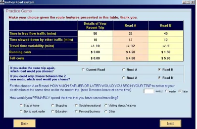
The data used in this study are drawn from a study conducted in Australia in2004, in the context of car driving non-commuters making choices from a range of level of service packages dened in terms of travel times and costs, including a toll where applicable. The choice scenarios presented respondents with 16 choice sets, each giving a choice between their current (reference) route and two alternative (unlabelled) routes with varying trip attributes (based around the reference trip). A statistically ecient design that is pivoted around the knowledge base of travellers is used to establish the attribute packages in each choice scenario. The trip attributes associated with each route are free ow time (FFT), slowed down time (SDT) caused by congestion, trip time variability (VAR), running cost (RC) and toll cost (TOLL). An example of a choice scenario (from a practice game) is shown in Figure1. For the present analysis, we made use of a sample of 3,792observations from 237respondents travelling for non-commute reasons. After completion of the 16 choice tasks, each respondent was presented with a screen capturing information on attribute processing, as shown in Figure 2. In particular, each respondent was asked to indicate whether they had ignored any of the ve attributes in making their choices, and whether the two time components and/or the two cost components had been treated separately or jointly. Finally, respondents were also asked to rank the ve attributes in order of importance.
3.2 Model specication
Three dierent models were estimated on the data, two MMNL models and the hybrid model shown in Equation 13. All three models were coded in Ox 6.2 (Doornik, 2001), using 500 MLHS draws per respondent and per random term in simulation based estimation (cf. Hess et al.,2006). For the hybrid model, simultaneous estimation of all model components was used.
In the rst MMNL model (MMNL1), constants were included for the rst two alternatives (ASC1and
ASC2). All ve marginal utility coecients were specied to vary randomly across respondents, where
Figure 1: An example of a stated choice screen
[image:9.612.108.506.364.639.2]Normal variates that are distributed independently and identically across respondents, draws for the ve marginal utility coecients are given by:
βFFT=−eµln(−βFFT)+s11ξ1
βSDT=−eµln(−βSDT)+s21ξ1+s22ξ2
βVAR=−eµln(−βVAR)+s31ξ1+s32ξ2+s33ξ3
βRC=−eµln(−βRC)+s41ξ1+s42ξ2+s43ξ3+s44ξ4
βTOLL=−eµln(−βTOLL)+s51ξ1+s52ξ2+s53ξ3+s54ξ4+s55ξ5
, (14)
whereskl(with l≤k≤5) relate to the Cholesky terms of the underlying Normal distribution, while e.g. µln(−βFFT) gives the mean for the underlying Normal distribution for the free ow time coecient.
In the second MMNL model (MMNL2), we allow for two dierent values for each coecient,
depend-ing on whether a respondent indicated that he/she attended to that attribute or not. For a respondent who indicated that he/she attended only to a subset of the attributes, the utility function will make use of coecients from the rst group (attending) for those attributes that were said to have been attended to, and coecients from the second group (non-attending) for the remainder. This model thus uses the respondent reported processing strategies as error-free explanatory variables, and also puts us at risk of biased results due to correlation between these indicators and other unexplained eects. The model is primarily included for illustrative purposes given its past use in the literature, and despite the issues discussed above. No attempts were made to additionally incorporate deterministic eects linked to the respondent reported attribute rankings. The second MMNL model makes use of 20 additional parameters, using two versions of the marginal utility coecients (along with the full Cholesky matrix), one for the attendance group and one of the non-attendance group.
In the hybrid model, we make use of the non-attendance data as well as the ranking data from Figure
2, with likelihood contributions given in Equation 7 and 12. Attempts to include socio-demographic interactions in the latent variable specication in Equation5were unsuccessful, but remain an important area for future work. In comparison with the rst MMNL model, the hybrid model makes use of 24 additional parameters, ve of them in the choice model (the λ terms), with the remaining 19 being used in the measurement model. This latter model is appropriately normalised and this is the most parsimonious suitable specication, such that there is no risk of overtting.
The veλparameters quantify the eect of the latent variables inside the choice model, as shown in Equation 8. With α following a standard Normal distribution, we can see that the β parameters in the hybrid model thus still follow a Lognormal distribution, just as in the base model. In particular, we have that:
βn,FFT =−eλFFTαn,FFTe µln(−β
FFT)+s11ξ1
βn,SDT =−eλSDTαn,SDTe µln(−β
SDT)+s21ξ1+s22ξ2
βn,VAR =−eλVARαn,VARe µln(−β
VAR)+s31ξ1+s32ξ2+s33ξ3
βn,RC =−eλRCαn,RCe µln(−β
RC)+s41ξ1+s42ξ2+s43ξ3+s44ξ4
βn,TOLL =−eλTOLLαn,TOLLe µln(−β
TOLL)+s51ξ1+s52ξ2+s53ξ3+s54ξ4+s55ξ5
. (15)
The remaining sets of parameters (κ,ζ,ς andτ) follow the approach set out in Equations7 and10 to
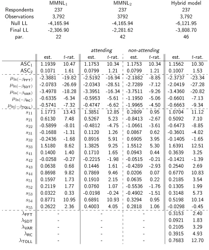
Table 1: Estimation results (part 1)
MMNL1 MMNL2 Hybrid model
Respondents 237 237 237
Observations 3,792 3792 3,792
Null LL -4,165.94 -4,165.94 -6,121.95
Final LL -2,306.90 -2,281.62 -3,808.70
par. 22 42 46
attending non-attending
est. t-rat. est. t-rat. est. t-rat. est. t-rat. ASC1 1.1939 10.47 1.1753 10.34 1.1753 10.34 1.1562 10.30
ASC2 0.1071 1.61 0.0799 1.21 0.0799 1.21 0.1007 1.53
µln(−βFFT) -2.3881 -19.82 -2.5192 -16.94 -2.1882 -8.85 -2.3737 -23.34
µln(−βSDT) -2.0783 -26.69 -2.0343 -28.51 -2.7289 -7.12 -2.0419 -27.28
µln(−βVAR) -3.4978 -18.28 -3.3951 -16.34 -3.7511 -9.26 -3.4360 -20.82
µln(−βRC) -0.6335 -6.34 -0.5953 -5.61 -1.1950 -5.06 -0.6601 -7.13
µln(−βTOLL) -0.5741 -7.32 -0.4747 -6.62 -1.9965 -4.50 -0.6663 -9.34
s11 1.1773 13.43 1.3851 12.85 0.2809 0.95 1.0704 11.12
s21 0.6130 7.48 0.5267 5.23 -0.8413 -2.67 0.5092 7.10
s22 -0.5899 -8.01 -0.4812 -4.75 -1.0661 -3.61 -0.6473 -8.85
s31 -0.1688 -1.31 0.1120 1.26 0.0867 0.62 -0.3601 -4.02
s32 -0.2436 -1.68 0.8916 5.91 0.6905 3.95 -0.1405 -1.65
s33 1.5180 8.62 1.3825 9.25 1.5512 5.30 1.6391 12.51
s41 0.1400 1.40 0.1710 1.65 0.0943 0.44 0.3639 3.25
s42 -0.0258 -0.27 -0.2215 -1.98 -0.0515 -0.21 -0.1421 -1.39
s43 0.0638 0.68 0.1446 1.61 -0.4289 -2.93 0.2540 2.69
s44 0.8698 9.82 0.7869 9.46 0.0206 0.07 0.6770 10.83
s51 0.1597 1.73 0.1910 2.15 0.0635 0.22 0.2185 3.54
s52 0.2119 1.77 0.0760 1.07 -0.5536 -1.76 0.1305 1.99
s53 0.0322 0.33 -0.0198 -0.24 -0.4902 -1.51 0.3148 5.73
s54 0.8771 10.95 0.6891 10.93 0.3294 0.95 0.5198 10.14
s55 0.2622 2.36 0.4003 4.05 0.2818 1.06 -0.0298 -0.45
λFFT - - - 0.3153 2.40
λSDT - - - 0.0921 1.83
λVAR - - - 0.2105 3.29
λRC - - - 0.3915 4.93
λTOLL - - - 0.7683 12.70
3.3 Results
The rst part of the estimation results are summarised in Table 1. They relate to model statistics and the estimates of the discrete choice component of the three models. We rst note that MMNL2 obtains
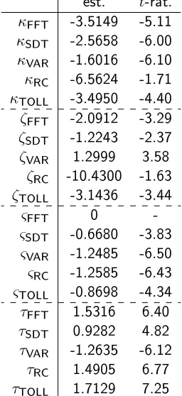
Table 2: Estimation results (part 2)
est. t-rat. κFFT -3.5149 -5.11 κSDT -2.5658 -6.00 κVAR -1.6016 -6.10 κRC -6.5624 -1.71 κTOLL -3.4950 -4.40 ζFFT -2.0912 -3.29 ζSDT -1.2243 -2.37 ζVAR 1.2999 3.58 ζRC -10.4300 -1.63 ζTOLL -3.1436 -3.44
ςFFT 0
-ςSDT -0.6680 -3.83 ςVAR -1.2485 -6.50 ςRC -1.2585 -6.43 ςTOLL -0.8698 -4.34 τFFT 1.5316 6.40 τSDT 0.9282 4.82 τVAR -1.2635 -6.12 τRC 1.4905 6.77 τTOLL 1.7129 7.25
20additional parameters. The t of the hybrid model cannot be compared to that of the MMNL models given the latter are estimated on the stated choice data alone, while the hybrid structure also models the responses to the non-attendance questions and the attribute ranking questions. This is reected in the greater null log-likelihood (LL) for the hybrid model.
Looking at the actual estimates, we see that the values for the two alternative specic constants indicate some inertia towards the reference attendance, along with some reading left-to-right eects. The ve mean parameters for the underlying Normal distributions are all statistically signicant across all three models. In MMNL2, the estimates for the underlying mean parameters are more negative in
the non-attendance set (except for free ow time), which translates into coecients with a median that is closer to zero (given the exponential), in line with the notion that these respondents have less strong sensitivities. For the Cholesky terms, the majority of estimates are also statistically signicant.
The nal set of estimates shown in Table 1 relate to the λ parameters, which have the role of a scaling parameter on the marginal utilities. Here, we see that for all ve attributes, increases in the associated latent variable lead to increases in sensitivity for the concerned attribute. This is line with the interpretation of the ve latent variables as underlying importance ratings for the attributes. As discussed in Section 2, the joint use of randomly distributed eλkαnk and β
k components would equate to an overspecication were it not for the use of αnk,∀k, in the remaining model components. In the present context, this can be most readily understood by noting again that the distribution ofeλkαnkβ
k is Lognormal, just as was the case for the distribution ofβk in the MMNL model (see alsoHess and Rose,
We next turn to the two additional model components that allow the use of theeλkαnk term, namely
the model for the response to the non-attendance questions, and the model for the response to the ranking question. The estimation results for the additional components for these components in the hybrid model are shown in Table 2.
We rst observe negative estimates for all κ parameters, where these reect the fact that the stated non-attendance rates were lower than 50% for each of the ve attributes. The ς terms for the ranking component play a similar role, where, with ςFFT normalised to zero, the remaining negative estimates reect the overall highest ranking for the free ow time attribute, ahead of slowed down time and tolls. Looking at the remaining parameters, a negative estimate for ζk would mean that asαnk increases, the probability of respondentnindicating that he/she ignored attributekis reduced. Similarly, a positive value forτk would mean that asαnk increases, the probability of respondentnranking attributekmore highly is increased.
Notwithstanding the reduced signicance for ζRC, we observe the expected sign for the ζ and τ parameters for free ow time, slowed down time, running costs, and tolls. Each time, an increase in the associated latent variable is associated with a reduced probability of stated non-attendance for that attribute, and an increased probability of higher ranking for the attribute (out of the set of5attributes). At the same time, the estimates for the λ parameters in the choice model component show that such increases in the latent variables also lead to heightened sensitivity to the associated attributes in the utility functions. This thus indicates consistent results across the three model components for these four attributes and justies the interpretation of the latent variable as an underlying attribute importance rating.
However, a dierent picture emerges for trip time variability. Here, the estimate forλVARin the choice model is once again positive, indicating that increases in the latent variable lead to increased marginal disutilities for the trip time variability attribute. However, the estimate for ζVAR is positive, while the estimate forτVARis negative. This thus indicates that increases in the latent variableαn,VAR, which lead to increases in the marginal disutility for trip time variability, also equate to a higher probability of stated non-attendance for this attribute, and increased probability of a lower ranking for the attribute.
These results for trip time variability thus highlight a lack of consistency between the behaviour in the stated choice components and the respondent provided information on attribute non-attendance and attribute ranking. Hess and Hensher (2010) had already observed a lack of correspondence between stated and inferred ignoring strategies for the variability attribute, which could help explain this. It also further highlights the usefulness of the modelling framework set out in this paper as it allows for such discrepancies to be identied, without relying on deterministic approaches treating respondent provided information as error free measures of attribute non-attendance and attribute rankings.
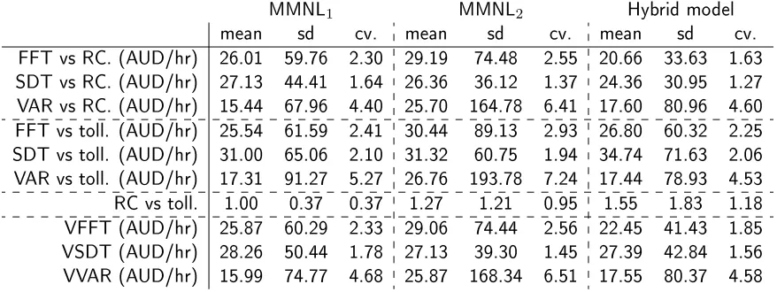
As a nal step, we calculate trade-os between coecients, with results summarised in Table 3. In particular, we calculate the monetary valuations for the three travel time components, using either running costs or tolls as the cost component. We also look at the distribution of the relative sensitivity to running costs and tolls. Finally, we show the willingness to pay distributions obtained by using a weighted average of the ratios against running costs and tolls, based on the relative distribution of the running cost and toll levels for the actual chosen alternative across all observations (labelled as VFFT, VSDT, and VVAR). In the MMNL model, the βk parameters all follow Lognormal distributions with the same applying to the eλkαnkβ
Table 3: Implied trade-os and monetary valuations
MMNL1 MMNL2 Hybrid model
mean sd cv. mean sd cv. mean sd cv. FFT vs RC. (AUD/hr) 26.01 59.76 2.30 29.19 74.48 2.55 20.66 33.63 1.63 SDT vs RC. (AUD/hr) 27.13 44.41 1.64 26.36 36.12 1.37 24.36 30.95 1.27 VAR vs RC. (AUD/hr) 15.44 67.96 4.40 25.70 164.78 6.41 17.60 80.96 4.60 FFT vs toll. (AUD/hr) 25.54 61.59 2.41 30.44 89.13 2.93 26.80 60.32 2.25 SDT vs toll. (AUD/hr) 31.00 65.06 2.10 31.32 60.75 1.94 34.74 71.63 2.06 VAR vs toll. (AUD/hr) 17.31 91.27 5.27 26.76 193.78 7.24 17.44 78.93 4.53 RC vs toll. 1.00 0.37 0.37 1.27 1.21 0.95 1.55 1.83 1.18 VFFT (AUD/hr) 25.87 60.29 2.33 29.06 74.44 2.56 22.45 41.43 1.85 VSDT (AUD/hr) 28.26 50.44 1.78 27.13 39.30 1.45 27.39 42.84 1.56 VVAR (AUD/hr) 15.99 74.77 4.68 25.87 168.34 6.51 17.55 80.37 4.58
the distributions of α andβ, as well as the distribution of stated non-attendance in MMNL2.
Overall, the dierences between MMNL1 and the hybrid model are relatively modest. However, we
observe larger (and arguably more realistic) dierences between the monetary valuations of free ow time and slowed down time in the hybrid model than was the case in MMNL1. It is also notable that for the
majority of trade-os, we see reduced heterogeneity in the hybrid model, with the main exception being the distribution of the relative sensitivity to running costs and tolls. This reduced and more realistic level of heterogeneity is arguably a reection of a greater ability by this model to accommodate the heterogeneity across respondents by linking the values to underlying attribute importance ratings, where this is not possible in MMNL1 which does not make use of the additional information. Further interesting
observations can be reached by comparing MMNL1and MMNL2. Here, we arguably observe more realistic
results in MMNL1, noting for example the wrong ordering between FFT and SDT in MMNL2, as well as
an excessive level of heterogeneity in the valuation of travel time variability. It could be argued that these ndings point to underlying aws in a model that deterministically conditions on respondent reported processing strategies.
4 Conclusions
There is now a large body of research looking at ways of accounting for possible heterogeneity across respondents in the way in which individual attributes are processed in a decision making context. Recent work has focussed on attempting to infer such processing strategies from the data rather than relying on respondent provided information, although the latter is still widespread too, especially outside the transport literature. The two main arguments against using respondent provided information on process-ing strategies are the possible endogeneity bias, and concerns about the empirical correctness of such respondent provided information. Indeed, repeated empirical evidence has suggested that respondents who indicate that they ignored a certain attribute still show a non-zero sensitivity to that attribute, albeit one that is lower than for the remaining respondents.
underlying unobserved importance rating which inuences the marginal utilities in the choice model as well as the answers to direct questions about processing strategies. This means that the answers to such questions are treated correctly as dependent variables rather than explanatory variables.
Our empirical application has shown that the proposed model performs well on a typical stated choice dataset. In particular, we have shown how there is a high level of consistency between the answers to processing questions concerning four of the ve attributes, and the marginal utilities for these attributes in the choice model. Crucially, with the presence of a random component in the latent variable, the model does not assume a one-to-one relationship and thus allows for dierences between actual and stated processing strategies. Furthermore, we use a coecient scaling approach rather than setting the coecient to zero at a certain threshold for the latent variable. Our analysis has also revealed some modest impacts on implied willingness to pay patterns, with a more realistic dierence between the valuations for free ow time and slowed down time, and lower overall heterogeneity. Finally, it is worth mentioning again that, unlike approaches using respondent reported processing strategies as explanatory variables, our method does not expose an analyst to the same risk of endogeneity bias. After estimation, the model can also be applied without the additional measurement model components, i.e. not making use of the data on processing strategies, which is clearly not possible in the deterministic model. A comparison with a model conditioning on stated processing strategies seems to indicate that our proposed structure produces more realistic results.
An interesting observation in our example relates to the fth attribute, namely trip time variability. Here, we see that increases in the latent variable lead to heightened marginal disutilities in the choice model, but higher probability of stated non-attendance and lower attribute ranking. This thus shows a misalignment between the stated processing strategies for that attribute and the actual behaviour in the data, an observation also supported by earlier discussions inHess and Hensher(2010). We attribute this evidence to the form of the trip time variability attribute. More recent studies have moved away from using a plus/minus travel time variability attribute, and instead use an attribute dened by a number of travel times and occurrence probabilities over a predened number of repeated trips for the exact same trip. Thus although there is merit in including the travel time variability attribute in the present analysis since it was included in the survey, we are inclined to put little emphasis on the substantive empirical nding. This does not impact on the main contribution of this paper.
While promising, the results from this paper relate to a single dataset, and future studies should conrm the applicability of the model to other datasets. Further work is also required to establish the impact of socio-demographics on the latent attribute importance ratings. Other functional forms for the measurement model could also be explored, where it would also be of interest to look at the role that the actual values of the attributes have on the responses to the processing questions. Finally, as alluded to in the introduction, numerous other dimensions of interest beyond attribute non-attendance exist in the eld of research into processing strategies, and latent variable models such as the one put forward in this paper are potentially of great use in such areas too.
Acknowledgements
References
Alemu, M. H., Mørbak, M. R., Olsen, S. B., Jensen, C. L., 2011. Attending to the reasons for attribute non-attendance in choice experiments. paper presented at the Second International Choice Modelling Conference, Oulton Hall, Leeds.
Balcombe, K., Burton, M., Rigby, D., 2011. Skew and attribute non-attendance within the bayesian mixed logit model. paper presented at the Second International Choice Modelling Conference, Oulton Hall, Leeds.
Ben-Akiva, M., Walker, J., Bernardino, A., Gopinath, D., Morikawa, T., Polydoropoulou, A., 2002. Integration of choice and latent variable models. In: Mahmassani, H. (Ed.), In Perpetual motion: Travel behaviour research opportunities and application challenges. Pergamon, Ch. 13, pp. 431470. Bolduc, D., Ben-Akiva, M., Walker, J., Michaud, A., 2005. Hybrid choice models with logit kernel:
Applicability to large scale models. In: Lee-Gosselin, M., Doherty, S. (Eds.), Integrated Land-Use and Transportation Models: Behavioural Foundations. Elsevier, Oxford, pp. 275302.
Cameron, T., DeShazo, J., 2011. Dierential attention to attributes in utility-theoretic choice models. Journal of Choice Modelling 3 (3), 73115.
Cantillo, V., Heydecker, B., Ortúzar, J. de D., 2006. A discrete choice model incorporating thresholds for perception in attribute values. Transportation Research Part B 40 (9), 807825.
Carlsson, F., Kataria, M., Lampi, E., 2010. Dealing with Ignored Attributes in Choice Experiments on Valuation of Sweden's Environmental Quality Objectives. Environmental & Resource Economics 47 (1), 6589.
Doornik, J. A., 2001. Ox: An Object-Oriented Matrix Language. Timberlake Consultants Press, London. Hensher, D. A., 2006. How do respondents handle stated choice experiments? - attribute processing
strategies under varying information load. Journal of Applied Econometrics 21, 861878.
Hensher, D. A., 2008. Joint estimation of process and outcome in choice experiments and implications for willingness to pay. Journal of Transport Economics and Policy 42 (2), 297322.
Hensher, D. A., 2010. Attribute processing, heuristics and preference construction in choice analysis. In: Hess, S., Daly, A. J. (Eds.), State-of Art and State-of Practice in Choice Modelling: Proceedings from the Inaugural International Choice Modelling Conference. Emerald, Bingley, UK, Ch. 3, pp. 3570. Hensher, D. A., Rose, J. M., Greene, W. H., 2005. The implications on willingness to pay of respondents
ignoring specic attributes. Transportation 32 (3), 203222.
Hess, S., Hensher, D. A., 2010. Using conditioning on observed choices to retrieve individual-specic attribute processing strategies. Transportation Research Part B 44 (6), 781790.
Hess, S., Rose, J. M., 2012. Can scale and coecient heterogeneity be separated in random coecients models? Transportation forthcoming.
Hess, S., Train, K., Polak, J. W., 2006. On the use of a Modied Latin Hypercube Sampling (MLHS) method in the estimation of a Mixed Logit model for vehicle choice. Transportation Research Part B 40 (2), 147163.
Hole, A. R., 2011a. A discrete choice model with endogenous attribute attendance. Economics Letters 110 (3), 203205.
Hole, A. R., 2011b. Attribute non-attendance in patients' choice of general practitioner appointment. paper presented at the Second International Choice Modelling Conference, Oulton Hall, Leeds. Hoyos, D., Mariel, P., Meyerho, J., 2011. Stated and inferred serial and choice task non-attendance in
choice experiments in the context of environmental valuation. paper presented at the Second Interna-tional Choice Modelling Conference, Oulton Hall, Leeds.
Puckett, S. M., Hensher, D. A., 2008. The role of attribute processing strategies in estimating the preferences of road freight stakeholders. Transportation Research Part E: Logistics and Transportation Review 44 (3), 379395.
Scarpa, R., Gilbride, T., Campbell, D., Hensher, D. A., 2009. Modelling attribute non-attendance in choice experiments for rural landscape valuation. European Review of Agricultural Economics 36 (2), 151174.