Towards a Three-Dimensional Phase-Field Model of Dendritic Solidification with Physically Realistic Interface Width

This is a repository copy of Towards a Three-Dimensional Phase-Field Model of Dendritic Solidification with Physically Realistic Interface Width.

White Rose Research Online URL for this paper: http://eprints.whiterose.ac.uk/74947/

Article:

Mullis, AM, Goodyer, CE and Jimack, PK (2012) Towards a Three-Dimensional

Phase-Field Model of Dendritic Solidification with Physically Realistic Interface Width. Transactions of the Indian Institute of Metals, 65 (6). 617 - 621 . ISSN 0972-2815 https://doi.org/10.1007/s12666-012-0181-2

[email protected] https://eprints.whiterose.ac.uk/

Reuse

See Attached

Takedown

If you consider content in White Rose Research Online to be in breach of UK law, please notify us by

Towards a 3-Dimensional Phase-Field Model of Dendritic Solidification with Physically Realistic Interface Width

A M Mullis†, C E Goodyer‡ and P K Jimack‡

Institute for Materials Research† and School of Computing‡, University of Leeds, Leeds LS2-9JT, UK.

Abstract

We review the application of advanced numerical techniques such as adaptive mesh refinement, implicit time-stepping, multigrid solvers and massively parallel implementations as a route to obtaining solutions to the 3-dimensional phase-field problem with a domain size and interface resolution previously possible only in 2-dimensions. Using such techniques it is shown that such models are tractable even as the interface width approaches the solute capillary length.

Keywords: Phase-field, dendritic growth, mesh adaptivity, multigrid methods.

Introduction

The modelling of solidification structures, in particular the growth of dendritic crystals, is a subject of intense and enduring interest within the scientific community, both because dendrites are a prime example of spontaneous pattern formation and they have a pervasive influence on the engineering properties of metals. However, in all but the most restrictive of cases, analytical solutions to the equations of motion for the solid-liquid interface, using techniques such as boundary integral methods (microscopic solvability theory [1]), cannot be found and recourse must be made to numerical techniques. One such technique which over the last few decades has received the most attention is that of phase-field simulation [2, 3], in which a non-conserved order parameter φ, which encodes the phase state of the material, is defined over the whole domain. By assuming the interface between the solid and liquid (or different solid phases in multi-phase modelling) to be diffuse, φ is rendered continuous, wherein standard techniques for partial differential equations (PDEs) may be used. This allows a regular Eulerian mesh to be used and avoids many of the topological complexities involved with front tracking methods.

However, phase-field modelling presents significant computational challenges in that the resulting set of PDE’s is highly non-linear and generally the width of the diffuse interface must be much narrower than the smallest physical feature to be simulated. This results in very large computational meshes, particularly when the problem is solved in 3-dimensions. The issue of mesh size arises because although the phase-field equations are formulated such that in the asymptotic limit of the diffuse interface width, W0, tending to zero, the corresponding sharp interface equations are recovered

exactly, this is not sufficient to ensure that the solutions do not have a dependence upon W0. Such limitations may be mitigated by formulating the model in the so-called

‘thin interface limit’ [4], whereby asymptotic expansions of the solution on the inner and outer regions of the solid-liquid interface are matched to obtain an equation set in

which dependencies which are linear in the diffuse interface width, W0, are eliminated.

However, dependencies which are of order , and higher, remain and consequently care still needs to be exercised in choosing W0 sufficiently small to ensure

convergence to a solution independent of W0. Moreover, in order to perform the

asymptotic matching highly restrictive assumptions need to be made about the thermodynamics governing the phase transformation, which can restrict the applicability of such models. Consequently, in many cases phase-field models are constructed such that W0 is much smaller than the other length scales characteristic of

the problem, wherein for W0sufficiently small convergence towards a solution

independent of W0 may be obtained. In the context of the models similar to that

described below, the effect of the interface width has been explored in 2-dimensions by [5, 6], from which it is clear that W0≈ 5d0 constitute the maximum interface width

wherein reliable solutions may be obtained, d0 being the chemical capillary length,

which is typically of the order 2–5×10−10 m. This compares with typical microstructural length scales which are of the order 10−6–10−5 m.

2 0 W

Due to this multi-scale nature phase-field simulations tend to be highly computationally intensive, requiring very significant spatial resolution in the vicinity of the (moving) phase interface. Consequently, much of the literature on phase-field simulation has tended historically to focus on two-dimensional problems, partly because such problems are generally tractable using simple numerical techniques such as explicit time stepping and uniform spatial meshing. However, even in two dimensions the limitations of such naive numerical approaches are well known and the advantages of using more sophisticated techniques, such as mesh adaptivity [7] and implicit time stepping [8], have been clearly demonstrated.

In this paper we describe the application to phase-field of a range of advanced numerical techniques, including dynamic mesh adaptivity, implicit temporal descretisation, non-linear multigrid solvers and parallel implementation that may move us towards making the problem of quantitative dendritic growth simulations in 3-dimensions with physically realistic interface widths tractable.

Mathematical Model

The phase-field model used here to illustrate the numerical techniques is that used by Echebarria et al. [ 9 ], in which, following non-dimensionalization against characteristic length and time scales, W0 and τ0, the evolution of the phase-field

equations is given by

⎥ ⎥ ⎥ ⎦ ⎤ ⎢ ⎢ ⎢ ⎣ ⎡ ⎟⎟ ⎟ ⎠ ⎞ ⎜⎜ ⎜ ⎝ ⎛ + ∂ ∂ + + ∇ ∂ ∂ ∂ ∂ + ⎥ ⎥ ⎥ ⎦ ⎤ ⎢ ⎢ ⎢ ⎣ ⎡ ⎟⎟ ⎟ ⎠ ⎞ ⎜⎜ ⎜ ⎝ ⎛ + ∂ ∂ + + ∇ ∂ ∂ − ∂ ∂ + ⎥ ⎦ ⎤ ⎢ ⎣ ⎡ ⎟⎟ ⎠ ⎞ ⎜⎜ ⎝ ⎛ + ∂ ∂ ∂ ∂ − + Ω − − + − + ∇ ⋅ ∇ = ∂ ∂ ∞ 2 2 2 2 2 2 2 2 2 2 2 2 2 2 2 2

2 _{( ) (1 ) (1 ) ( )}

y x y z y x y y x x z y x y y x A A A y A A A x A A z U Mc A t A φ φ φ φ ψ φ φ φ φ ϑ φ φ φ φ ψ φ φ φ φ ϑ φ φ ψ φ λ φ φ φ φ

with an anisotropy function A = A(ϑ,ψ) given in terms of the standard spherical angles, ϑ and ψ, by

(

)

[

]

{

}

) ,

(ϑψ = A₀ +ε 4ψ + 4ψ − 2ϑ 2ϑ

A

which corresponds to a preference for growth along the Cartesian coordinate axis. The small parameter ε governs the strength of the anisotropy, M is the scaled magnitude of the liquidus slope, c_∞ is the solute concentration far from the interface and Ω is a scaled superstauration given by

0 0 ) 1 ( _l l c k c c − − = Ω ∞

λ is a coupling parameter which determines the width of the diffuse interface, W0, via

the relation 2 0 0 1 a D d W a = =

λ , , 0.6267

8 2 5

2

1 = a =

a

where is the dimensionless solute diffusivity.

The evolution equation for the dimensionless concentration field, U, is given by

[

]

[

]

where k is the equilibrium partition coefficient. The non-dimensional concentration field, U, is related to the concentration, c, via

⎟⎟ ⎠ ⎞ ⎜⎜ ⎝ ⎛ − − + − = ∞ φ ) 1 ( 1 / 2 1 1 k k c c k

U .

Full details of the model used are given in [10, 11].

Numerical Methods

based upon the solution from the previous time level. In order to apply the FAS solver it is necessary to have a hierarchy of finite difference meshes so as to be able to resolve the solution at different length scales: we achieve this using nested hexahedral meshes which allow local mesh refinement and derefinement. This local adaptivity provides the necessary spatial resolution throughout the computational domain without requiring unnecessary degrees of freedom.

In order to control the three-dimensional mesh refinement and de-refinement we use the open source library, PARAMESH [14]. This library provides functions to generate meshes in an oct-tree structure of mesh blocks. Starting with a base block (of 8×8×8 cubic cells for example) it is possible to refine this into up to 8 child blocks (with each block always being of the same dimension as the base block) and then to refine any of these child blocks successively. Functions are also provided to undo regions of this local refinement (i.e. de-refinement) and to interpolate or restrict solution fields between meshes. A further capability of PARAMESH is that it is able to undertake this meshing in parallel in a manner that is hidden from the user – each block is simply treated as independent of its neighbours and PARAMESH takes care of which process owns each block, using its own dynamic load balancing scheme. A price that has to be paid for this simplicity is that every block is required to store guard cells in each dimension regardless of whether its neighbouring blocks are actually owned by a different process: PARAMESH’s guard cell update routines then take care of all of the transfer of data between neighbouring blocks, regardless of their location in memory.

The use of PARAMESH imposes a number of constraints upon our choice of finite difference stencil. Specifically, we avoid the use of any points around cell (i, j, k) that are not of the form (i±1, j±1, k±1) as this ensures that our parallel implementation needs only a single layer of guard cells between blocks of the mesh that are stored on different processors – which reduces the memory and communication overhead significantly. For the results reported here a compact 27-point stencil is used, which is found to significantly reduce mesh induced anisotropy relative to the standard 2nd order 7-point stencil in 3-dimensions.

The local refinement and de-refinement capability provided by PARAMESH is essential for this work since our phase-field models require very fine meshes around the solid-liquid interface in order to ensure that the interface is resolved with sufficient accuracy. The nondimensionalization used to derive the systems introduced in section 2 is such that the interface width is O(1) and so our mesh spacing cannot be greater than Δx = 1 around the interface. Hence the finest grid resolution needs to be at least this size (for a domain of dimension (0,400)×(0,400)×(0,400) at least nine levels of refinement are required, wherein 400/29 gives Δx = 0.78125 – though a tenth level is necessary if we wish to ensure that the interface is even moderately well resolved in its normal direction). Without the use of local mesh refinement and de-refinement there would need to be an excessive number of cells, creating a computational load that would be unmanageable without the very largest supercomputing resources, a uniform mesh with comparable resolution to our level 10 mesh here having > 1 billion elements.

As outlined above, the need for multigrid arises from our use of an unconditionally stable time-stepping scheme which result in a large system of nonlinear algebraic

equations at each time step. It has already been demonstrated in [8] that the use of implicit time-stepping for this particular phase-field model is essential for fine spatial resolution to be achieved, even in two space dimensions. This is because the stability constraints imposed on the time-step size by the small spatial mesh size at the phase boundary mean that explicit time-stepping is prohibitively slow. The extension of the PARAMESH capability to include nonlinear multigrid is explained in [ 15 ].The essential ingredients are the extension of the restriction and prolongation operators for the FAS scheme and for the use of the multi-step BDF formula (requiring data from previous time steps to be used at each multigrid level).

Results

Numerical validation of the model has been undertaken by comparing against the 3-dimensional adaptive explicit code due to Dantzig et al. [16]. For this test we used the following parameters; k = 0.15, Ω = 0.55, ε = 0.02 with D in the range 0.8 – 2.0, which corresponds to the interface width being in the range 1.4 – 3.6d0, broadly

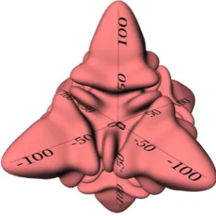
satisfying the stated condition that the width of the diffuse interface should be physically realistic, i.e. of the order a few atomic diameters. A typical dendrite morphology is shown in Fig. 1. Table 1 and Figure 2 give quantitative results of the comparison, in terms of the dimensionless tip radius, ρ/d0, and velocity, Vd0/D, for a

dendrite that has reached stead-state (i.e. the simulation has run for a sufficiently long time that no further variation in velocity or radius is observed with further growth). Good agreement is observed between the models in that for each value of D both the steady-state tip velocity and radius agree between the two models to within 5%. Due to computational limitations within the explicit code, which is also restricted to serial execution, we have run the comparison at a mesh spacing of Δx = 0.8, although given that D = 0.8, corresponds to W0 = 1.4 this is barely sufficient to resolve the diffuse

interface, so we have also used the implicit code to run a set of simulations for a more heavily refined mesh in which the minimum spacing is Δx = 0.4. Unfortunately, it was not possible to run a direct comparison for Δx = 0.4 using the explicit code as this potentially increases the computational time by a factor of 32 (there are up to 8 times as many elements in the mesh and due to the stability condition the time step needs to be reduced by a factor of 4 as the mesh spacing is halved). However, the results are generally encouraging in that the additional mesh refinement makes only a marginal difference to the results.

Perhaps more surprising is the extent to which both the velocity and tip radius vary as a function of the interface width. It is clear from Figure 2 that both the velocity and tip radius converge to a steady-state value in the implicit model as D is decreased towards D < 1 (corresponding to W0 < 1.8d0). In the explicit model the tip radius also

Figure 1. Typical 3-dimensional dendrite geometry produced by the phase-field model.

Method Δx Domain Dimensionless Velocity, Vd0/D

D = 0.8 D = 1.0 D = 1.5 D = 2.0

Explicit 0.8 204.8 × 102.4 × 102.4 0.057 0.055 0.051 0.047

Implicit 0.8 204.8 × 102.4 × 102.4 0.057 0.056 0.051 0.046

Implicit 0.4 400 × 400 × 400 0.059 0.058 0.053 0.048

Dimensionless Radius, ρ/d0 D = 0.8 D = 1.0 D = 1.5 D = 2.0

Explicit 0.8 204.8 × 102.4 × 102.4 16.61 16.95 18.77 21.73

Implicit 0.8 204.8 × 102.4 × 102.4 17.70 17.79 19.52 21.63

Implicit 0.4 400 × 400 × 400 17.30 17.64 19.76 23.05

Table 1 - Comparison of the steady-state tip radius and velocity using the 3-d implicit software described here against an explicit 3-d code due to [16].

Figure 2. Variation of the dendrite tip velocity (open symbols, left-hand axis) and radius (solid symbols, right-hand axis) as a function of D, and hence of the diffuse interface width (W0≈ 1.8D). Note that quantitative convergence is only obtained close

to D≤ 1.

References

Summary & Conclusions

We have demonstrated that by using a range of advanced numerical techniques such as mesh adaptivity, implicit time-stepping and a non-linear multigrid solver, coupled with solution in parallel, it is feasible to use phase-field techniques to solve for the growth of a solutally controlled dendrite using a diffuse interface width comparable to the length scale over which crystalline order would be expected to be lost in the solid-liquid interface in metals. The model demonstrates that for interface widths larger than ≈ 2d0 (0.4-1.0 nm) it may be difficult to guarantee quantitatively valid results,

which posses severe computational challenges for 3-dimensional phase-field models, particularly those using explicit temporal descretisation schemes.

1. Barbieri A, and Langer J S, Phys. Rev. A39 (1989) 5314.

2. Langer J S, in Directions in condensed matter physics, (eds) Grinstein G, Mazenko G,World Scientific Publishing, Singapore, (1986) p 164. 3. Penrose O, and Fife P C, Physica D43 (1990) 44.

4. Karma A, and Rappel W-J, Phys. Rev. E53 (1996) R3017. 5. Ramirez JC and Beckermann C, Acta Mater.53 (2005) 1721. 6. Mullis AM, J. Cryst. Growth312 (2010) 1891.

7. Provatas N, Goldenfeld N, and J. Dantzig, J. Comput. Phys.148 (1999) 265. 8. Rosam J, Jimack P K, Mullis A M, J. Comput. Phys.225 (2007) 1271.

9. Echebarria B, Folch R, Karma A and Plapp M, Phys. Rev. E70 (2004) 061604. 10. Rosam J, Jimack P K, Mullis A M, Acta Mater. 56 (2008) 4559.

11. Goodyer C E, Jimack P K, Mullis A M, Dong H, and Xie Y, Adv. Appl. Math. Mech. in press.

12. Hundsdorfer W, and Verwer J G, Numerical Solution of Time-Dependent Advection-Diffusion-Reaction Equations. Springer, Verlag (2003).

13. Brandt A, Math. Comput.31 (1977) 333.

14. Olson K, in Parallel Computational Fluid Dynamics 2005: Theory and Applications, (ed) Deane A, Brenner G, Emerson DR, McDonough J, Tromeur-Dervout D, Satofuka N, Ecer A, Periaux J, Elsevier, 2006.

15. Green J R, Jimack P K, Mullis A M, Rosam J, Partial Differential Eq, 27 (2011) 106.