White Rose Research Online URL for this paper:
http://eprints.whiterose.ac.uk/136192/
Version: Published Version
Monograph:
Saramago Goncalves, Pedro Rafael orcid.org/0000-0001-9063-8590, Chuang,
Ling-Hsiang and Soares, Marta Ferreira Oliveira orcid.org/0000-0003-1579-8513 (2014)
Network meta-analysis of (individual patient) time to event data alongside (aggregate)
count data. Discussion Paper. CHE Research Paper . Centre for Health Economics,
University of York , York, UK.
[email protected] https://eprints.whiterose.ac.uk/
Reuse
Items deposited in White Rose Research Online are protected by copyright, with all rights reserved unless indicated otherwise. They may be downloaded and/or printed for private study, or other acts as permitted by national copyright laws. The publisher or other rights holders may allow further reproduction and re-use of the full text version. This is indicated by the licence information on the White Rose Research Online record for the item.
Takedown
If you consider content in White Rose Research Online to be in breach of UK law, please notify us by
Network Meta-Analysis of (Individual
Patient) Time to Event Data alongside
(Aggregate) Count Data
Network meta-analysis of (individual patient) time to
event data alongside (aggregate) count data
1
Pedro Saramago
2
Ling-Hsiang Chuang
1
Marta Soares
1
Centre for Health Economics, University of York, UK
2
Pharmerit International, Rotterdam, The Netherlands
CHE Discussion Papers (DPs) began publication in 1983 as a means of making current research material more widely available to health economists and other potential users. So as to speed up the dissemination process, papers were originally published by CHE and distributed by post to a worldwide readership.
The CHE Research Paper series takes over that function and provides access to current research output via web-based publication, although hard copy will continue to be available (but subject to charge).
Disclaimer
Papers published in the CHE Research Paper (RP) series are intended as a contribution to current research. Work and ideas reported in RPs may not always represent the final position and as such may sometimes need to be treated as work in progress. The material and views expressed in RPs are solely those of the authors and should not be interpreted as representing the collective views of CHE research staff or their research funders.
Further copies
Copies of this paper are freely available to download from the CHE website www.york.ac.uk/che/publications/ Access to downloaded material is provided on the understanding that it is intended for personal use. Copies of downloaded papers may be distributed to third-parties subject to the proviso that the CHE publication source is properly acknowledged and that such distribution is not subject to any payment.
Printed copies are available on request at a charge of £5.00 per copy. Please contact the CHE
Publications Office, email [email protected], telephone 01904 321405 for further details.
Centre for Health Economics Alcuin College
University of York York, UK
www.york.ac.uk/che
Abstract
Objectives: Network meta-analysis (NMA) methods extend the standard pair-wise framework to allow simultaneous comparison of multiple interventions in a single statistical model. Despite published work on NMA mainly focussing on the synthesis of aggregate data (AD), methods have been developed that allow the use of individual patient-level data (IPD) specifically when outcomes are dichotomous or continuous. This paper focuses on the synthesis of IPD and AD time to event data, motivated by a real data example looking at the effectiveness of high compression treatments on the healing of venous leg ulcers.
Methods: This paper introduces a novel NMA modelling approach that allows IPD (time to event with censoring) and AD (event count for a given follow-up time) to be synthesised jointly by assuming an underlying, common, distribution of time to healing. Alternative model assumptions were tested within the motivating example. Model fit and adequacy measures were used to compare and select models.
Results: Due to the availability of IPD in our example we were able to use a Weibull distribution to describe time to healing; otherwise, we would have been limited to specifying a uniparametric distribution. Absolute effectiveness estimates were more sensitive than relative effectiveness estimates to a range of alternative specifications for the model.
1.
Background
In clinical practice, and at a wider societal level, treatment decisions in medicine need to consider all relevant alternative health care technologies. Such decisions are ideally informed by evidence on the relative effectiveness of treatments generated by randomised controlled trials (RCTs) (which may be further used to inform estimates of cost-effectiveness). Using evidence from individual RCTs may limit informed decision making since studies usually only provide comparative evidence on two treatments, potentially missing other relevant technologies which are also treatment options. This limitation can be overcome if all RCTs evaluating interventions relevant to the treatment decision are considered collectively, for example, with the use of network meta-analysis (NMA). NMA is a well-established statistical technique that extends standard the pairwise meta-analysis framework to allow simultaneous comparison of multiple interventions in a single statistical model. (1, 2) This approach then produces relative effect estimates (and associated descriptions of uncertainty) for all treatments connected by the network of evidence even where head-to-head trials for comparisons do not exist (indirect data).
NMA using individual patient data
Published work on NMA mainly focuses on the synthesis of aggregate data (AD) (sometimes called summary data, e.g. group means and standard errors available from study reports) (3, 4); however, methods have been developed that allow use of individual patient-level data (IPD) in NMA (5-7). The appeal of including IPD in a NMA is that it is likely to reduce statistical heterogeneity across the network (and in this way help resolve possible inconsistencies); and it may also allow for subgroup effects to be estimated that could guide more personalised treatment decisions (5). The use of IPD, alone or in combination with AD, has been shown to improve inference in NMAs where the outcome of interest is dichotomous (or binary) by aiding convergence, and by providing unbiased treatment covariate interactions [that would otherwise be affected by ecological bias (8)]. For continuous outcomes, IPD is likely to also lead to more precise estimates of treatment effects, even in the absence of treatment covariate interactions (9).
NMA using time to event related outcome data
Where individual studies present hazard ratios, these AD can be pooled directly using standard methods (analogous to pooling count data where relative effectiveness measures are the odds ratios or relative risks) (10). However, other AD outputs such as median/mean time to event (11) and cumulative counts of patients having the outcome event in a period of time (12) have also been meta-analysed in a network by specifying an underlying time to event distribution hazard ratios can be generated from these outputs (13). Whereas IPD having been used in pairwise analysis (12), there has been limited development of methods in the NMA framework.
Developing a NMA combining AD and IPD data to synthesise time to event related outcomes
2.
Motivating example: high compression treatments for venous leg ulcers
T
mmHg compression at the ankle) to promote venous leg ulcer healing. Available standardised systems are: two layer hosiery (HH), the four layer bandage (4LB), the short stretch bandage (SSB), the zinc paste bandage (ZINC), and the two layer bandage system (2LB). A detailed description is provided in Box A1 in Appendix with further details of these systems presented elsewhere (14).
Effectiveness evidence from RCTs was obtained from the most recent update of the relevant Cochrane review available to us (15), and from a recent multicentre RCT which compared 4LB with HH. All available RCT evidence was assessed for inclusion in the current NMA: a detailed process that has been reported elsewhere (14). The final NMA contained data from 16 RCTs on the relative effectiveness of high compression systems for the treatment of venous leg ulcers. Data for two of the 16 included RCTs (VenUS I and VenUS IV, hereby denominated studies 1 and 2) had full IPD data available (841 participants) which included time to healing or censoring for each participant, together with other individual-level characteristics such as treatment centre, ulcer duration and size and also patient mobility. For the remaining RCTs (1105 participants), aggregate data on the number of healed ulcers were extracted from the source review alongside information regarding treatment type, number of participants allocated to each treatment group, mean duration of follow-up (if this was not stated, trial duration was used), mean ulcer duration and size.
The 16 included RCTs described nine unique high compression treatments: the five standard
treatments (4LB, SSB, ZINC, HH and the 2LB) and four ad hoc systems (14). The ad hoc group
consisted of treatments deemed irrelevant to current clinical practice, and are not reported further (results can be provided upon request). These studies were, however, included in the NMA as their data may still be relevant, for example, in describing determinants of healing.
Table 1: Analytic dataset ID Study Treatment Follow up (weeks) Number patients Mean duration (months) Mean size (cm2)
Number healed
Evidence format available
16 Duby et al 1993 (16) 4LB 12 25 20.5 11.9 11
AD
SSB 12 25 26.7 13.1 10
17 Scriven et al 1998 (17) 4LB 52 32 13 13.3 17.6
AD
SSB 52 32 21 8.3 18.24
18 Partsch et al 2001 (18) 4LB 16 53 1.25 1.5 33
AD
SSB 16 59 1 1.9 43
19 Ukat et al 2003 (19) 4LB 12 44 -- 17.7 13
AD
SSB 12 45 -- 12.2 10
20 Franks et al 2004 (20) 4LB 24 74 2 5 59
AD
SSB 24 82 2 3.5 62
21 Junger et al 2004b (21) SSB 12 60 5.57 5.95 19
AD
HH 12 61 4.14 5.62 29
22 Kralj et al 1996 (22) 4LB 24 20 7.9 18.6 7
AD
Ad hoc: Ba 24 20 6.9 17.2 8
23 Polignano (23) et al 2004b 4LB 24 39 -- 10.1 29 AD
ZINC 24 29 -- 9.3 19
24 Wilkinson (24) et al 1997 4LB 12 17 -- 11.2 8
AD
Ad hoc:
BHeH 12 18 -- 8.6 8
25 Colgan et al 1995 (25) 4LB 12 10 9.3 27.5 6
AD
Ad hoc:
BzeaH 12 10 66.5 48.5 7
26 Blecken et al 2005 (26) 4LB 12 12 -- 50.08 4
AD
Ad hoc: HV 12 12 -- 48.98 4
27 Moffatt et al 2008 (27) 4LB 4 42 48.8 5.7 3
AD
2LB 4 39 46.6 11.8 6
28 Szewczyk (28) et al 2010 4LB 12 15 -- 6 9
AD
2LB 12 16 -- 5.3 10
29 Wong et al 2012 (29) 4LB 24 107 -- -- 72
AD
SSB 24 107 -- -- 77
30 Iglesias et al 2004 (30) 4LB 52 195 3 3.81 107
IPD
SSB 52 192 3 3.82 86
14 Ashby et al 2013 (14) 4LB 52 224 12.29 9.30 157
IPD
HH 52 230 10.82 9.41 163
Figure 1: Network of RCTs
In the network, a unique treatment category is indicated by a circle. Arrows between circles indicate that these
ID T
(4LB, SSB, HH, Ba, Zinc paste, BHeH, BzeaH, HV and 2LB as described in Box A1 in Appendix)
AD: [27-28]
AD: [24] AD: [22]
AD: [25] AD: [16-21]
IPD1: [30]
AD: [23] AD: [26] AD: [29]
HH
4LB
BzeaH
ZINC SSB
BHeH
2LB
HV Ba Ad-hoc treatments
3.
Methods
We first describe in detail the modelling framework for our main analysis, model A. We then detail
the process of evaluating alternative assumptions to this model, thus highlighting and challenging specific assumptions of the modelling framework proposed. All synthesis was conducted in a Bayesian framework.
3.1.
Statistical model for the data
We describe model A in two interrelated parts [analogous to Sutton et al (31) and Saramago et al
(5)]: part I describes the modelling of the IPD and part II the modelling of the AD.
Model A, part I- modelling the IPD studies, controlling for baseline covariates
(A1)
Time to ulcer healing ( ) of the participant in the study and in the treatment arm was
assumed to be Weibull distributed (32) with shape1 parameter, s, and scale parameter, . For
some participants, time to event was not observed, and these observations were censored at the
time the participant last had trial data recorded, . The baseline hazard function, linear on the
log-scale, was modelled as a function of the log-hazard of an event for the baseline treatment b, , of
treatment effects, , and of a set of baseline regression terms, , where are the
covariate effects of a set of m (=4) regressors available in the IPD data sets (14): the log of the
baseline ulcer area and duration (in months) (both centred around its mean value); and two dummy
T hazard of healing were assumed to be equal
in both IPD studies (i.e. the coefficient of each covariate was constant). Due to the existence of missing covariate information for some individuals, a distributional assumption was imposed on the
covariate values, indicating that are Normally distributed with mean and precision ,
IPD T
2
, which enables the use of multiple imputation techniques through MCMC3. Additionally, to
account for centre variability within each IPD study, was defined for each centre, c, in the
study, these were combined using a common frailty effect, , described by a normal distribution with mean zero and precision .
The treatment effects, , were log-hazard ratios for treatment k relative to the study-specific
baseline treatment b, partitioned here as . Prior distributions were specified for
1
The shape parameter of the Weibull distribution, s, can be interpreted directly as follows: i) if 0 < s < 1, hazard rate decreases over time; ii) if s = 1, hazard rate is constant over time (hazard exponentially distributed); and if s > 1, it indicates that the hazard increases with time (Collet 2003).
2
The missing-at-random assumption (sometimes called the ignorability assumption) considers that the probability that an observation is missing may depend on the observed values but not the missing values, as sufficient data has already been collected.
3
, for each of the m regression coefficients , for
and , for the shared between centre variability
and for . Vague prior distributions were given to
. Note that , where A was treatment 4LB, arbitrarily chosen as reference
treatment.
Model A, part II - modelling the AD studies
(A2)
Within the AD studies, the observed number of participants with a healed study ulcer, , from the
total number of individuals in the trial and in the treatment arm (intention to treat), , was
assumed to be Binomially distributed. The underlying probabilities of an event for each arm and in
each trial were represented by . In turn, was expressed as a function of the hazard, , of
follow-up time, , and the shape parameter s. The hazard function, linear on the log-scale, was
modelled by the baseline log-hazard of an event for treatment b in study j, , and by the
log-hazard ratio for treatment k and baseline treatment b, . Note that there are
parameters common to both model parts (equations A1 and A2), namely the log-hazard ratios and the shape parameter of the time to healing distribution. Prior distributions were specified for
.
3.2.
Alternative modelling assumptions
A set of assumptions made within model A were challenged; these are detailed below.
Exploring between-study variation
Model A assumed that each included RCT aimed to measure a common treatment effect
(fixed-effect); however, it is likely that there was between-study variation. Model B included a random
effect to characterise between-study heterogeneity, by considering
rather than just this is common to both parts I (eq. A1) and II (eq. A2).
Time to healing distributions
Model A used the Weibull distribution to describe time to healing. Our choice of survival distribution was limited as distributions such as the Log-Logistic or the Log-Normal do not allow the probability of healing over time to be expressed in a closed form, and hence impede the approach proposed here for the joint synthesis of IPD and AD. Other distributions, such as the Gompertz, were not readily defined within the software used in this work (WinBugs/OpenBugs), specifically under censoring. Nonetheless, the goodness of fit could still be assessed in each IPD data source individually. To do so, we applied parametric regression survival-time models (32) to both IPD data
sources (16, 24) independently (covariates and frailty effect considered, as in model A).
Distributional shape parameter
the impact of this assumption on the relative effectiveness estimates: model C1 used the shape
parameter from the first IPD study to describe the AD studies and model C2 used the shape
parameter from the second IPD study (14) to describe these same studies. Because models C1 and
C2 represent simple modifications of model A we do not present these algebraically.
Treatment-covariate associations
Model A uses baseline covariates to adjust for clinical heterogeneity in the IPD. To further explore the impact of covariates on the relative treatment effects (i.e. whether they were effect modifiers), and potentially help explain between-study heterogeneity, we also included interaction terms
between alternative treatments and baseline ulcer area and duration as described by Cooper et al
2009 (33) and Saramago et al 2012 (5). Model D assumed a regression (slope) coefficient for the
interaction terms, this effect is common across treatments and thus common to parts I (eq. D1) and
II (eq. D2). This assumption was data driven, as this was the only option we were able to implement
(33). Note
that interaction estimates obtained are influenced by the full evidence base for which study mean
covariate(s) values are available, including trials considering ad hoc treatments. Given model D is
substantially different to model A we describe it algebraically here.
Model D, part I- modelling the IPD studies
(D1)
Time to ulcer healing is modelled in the same way as in
model A
. A set of
covariate-treatment interaction regression terms,
, are here defined, where
are the
association effects, assumed common across studies and the same regardless of treatment
(excluding control) , corresponding to a set
of n (=2) covariates including the log of the
baseline ulceration area and baseline ulcer duration (in months). For the remainder of the
parameters of interest, prior distributions were assigned as in
model A
.
Model D, part II - modelling the AD studies
(D2)
The underlying probabilities of an event for each arm in each trial, , were regressed against n
(=2) a set of study-level covariates [the log of the baseline ulceration area and baseline ulcer
duration (in months)]. Uninformative prior distributions were assigned to the regression coefficients,
, to and . All other components of the model
3.3.
Model selection and implementation
The NMA analyses were undertaken in the WinBUGs software (34). In all models the MCMC sampler
was run for 10 000 iterations and these were discarded as - Models were run for a further
5000 iterations, on which inferences were based. Chain convergence was checked. The WinBUGS code is included for reference in the Appendix. Within the NMA, goodness of fit was assessed using the deviance information criterion (DIC) (35). Results were presented using hazard ratio estimates (and associated credibility intervals, CrIs) and also using the probability of each compression system
ve (36).
4.
Results
Table 2 shows parameter estimates obtained for model A (first column) and alternative models
testing its assumptions (models B to D, second to fifth columns). The results for model A highlight
that the modelling framework proposed is feasible. The results of testing the assumptions are described next, in turn.
Exploring between-study variation
Despite estimates of HRs from the random effect model (model B) being associated with wider CrIs
than those from model A (as expected), point estimates were found to be fairly similar except for the
comparison between HH vs. 4LB: HH is estimated to be more effective in model B (HR 1.63, 95% CrI
0.76-3.53) compared to model A (HR: 1.05, 95% CrI 0.85 to 1.29), although the CrI of the former
includes the later. The treatment with the greatest estimated probability of healing was HH in model B (59%), rather than 2LB (72%) as in model A. Differences may be explained by any existing
variation between studies of SSB vs. 4LB indirectly impacting on the evidence loop 4LB vs. SSB vs.
HH. Baseline covariate effect estimates remained similar. However, note that the gain in quality fitting of the random-effects model compared to the fixed-effects is null (DIC: 5396.21 and 5396.22,
respectively). Previous published work assessing evidence on the SSB vs. 4LB comparison (39)
similarly found no evidence of between-study heterogeneity.
Time to healing distributions
The Weibull was the time to healing distribution used in model A. Whilst we were limited in the use
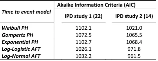
of other distributions, goodness of fit was explored by applying alternative time to event distributions to the IPD studies individually. Table 3 shows results of such analysis (AIC statistic). The best fitting distributions for both studies were the Log-Logistic and Log-Normal. Of the remaining, the Weibull and Gompertz distributions provided better fit than the Exponential; this was expected given the flexibility of these distributions in assuming increasing, decreasing or constant hazards over time. The Weibull was best in IPD study 2 and the Gompertz best in IPD study 1.
Distributional Weibull shape parameter of healing hazard
The Weibull shape parameters estimated within models C1 and C2 indicate that in IPD study 1 (30)
the hazard of healing was expected to decreases over time (sI = 0.93, 95% CrI 0.86-1.01), while in IPD
study 2 (14) it is expected to increase (s2 = 1.27, 95% CrI 1.17-1.38). Note that there is no overlap in
the CrIs. However, results show that relative effectiveness estimates are robust to the range of
assumptions tested: the estimated HRs did not differ between models C1 and C2, and did not
substantially differ from model A.
Treatment-covariate associations
Table 2: Parameter estimates from the alternative MTC synthesis models.
Model A Model B Model C1 Model C2 Model D
Hazard ratios HR median (95% CrI) P HR median (95% CrI) P HR median (95% CrI) P HR median (95% CrI) P HR median (95% CrI) P T re a tm e n t e ff e ct s
4LB --- --- 5.5 --- --- 1.4 --- --- 6.2 --- --- 5.7 --- --- 4.3
SSB 0.88 (0.76, 1.03) 0.4 0.96 (0.77, 1.22) 0.6 0.89 (0.77, 1.04) 0.6 0.89 (0.77, 1.04) 0.6 0.84 (0.70, 0.99) 0.2
HH 1.05 (0.85, 1.29) 16.1 1.63 (0.76, 3.53) 59.2 1.03 (0.83, 1.27) 14.9 1.03 (0.84, 1.27) 15.0 1.03 (0.84, 1.28) 11.1
ZINC 0.77 (0.41, 1.42) 6.2 0.78 (0.37, 1.62) 2.8 0.78 (0.41, 1.44) 6.5 0.78 (0.41, 1.43) 6.7 0.75 (0.03, 29.49) 17.5
2LB 1.40 (0.65, 3.05) 71.9 1.39 (0.62, 3.30) 36.0 1.38 (0.66, 3.05) 71.8 1.38 (0.63, 3.04) 72.0 1.59 (0.61, 5.34) 67.0 B a se li n e ch a ra ct e ri st ic
s Log area 0.71 (0.66, 0.76) --- 0.71 (0.66, 0.76) --- 0.70 (0.65, 0.75) --- 0.70 (0.65, 0.75) --- 0.71 (0.65, 0.76) ---
Log duration 0.92 (0.90, 0.94) --- 0.92 (0.90, 0.94) --- 0.92 (0.91, 0.94) --- 0.93 (0.91, 0.94) --- 0.92 (0.90, 0.94) ---
Difficulty in
walking 0.71 (0.60, 0.85) --- 0.73 (0.60, 0.86) --- 0.72 (0.60, 0.85) --- 0.72 (0.60, 0.85) --- 0.71 (0.60, 0.80) ---
Immobile 0.67 (0.23, 1.52) --- 0.66 (0.23, 1.51) --- 0.72 (0.24, 1.65) --- 0.72 (0.25, 1.67) --- 0.68 (0.24, 1.59) --- In te ra ct io n
s Log area --- --- --- --- --- --- --- --- --- --- --- --- 1.00 (0.97, 1.10) ---
Log duration --- --- --- --- --- --- --- --- --- --- --- --- 1.00 (0.99, 1.00) ---
Btw-centre SD 0.04 (0.01, 0.13) --- 0.05 (0.01, 0.13) --- 0.05 (0.01, 0.15) --- 0.05 (0.01, 0.15) --- ---
Btw-study SD --- --- --- 0.13 (0.01, 0.51) --- --- --- --- --- --- --- --- --- ---
1.07 (1.01, 1.13) --- 1.07 (1.01, 1.14) 1** 0.93 (0.86, 1.01) 1 0.93 (0.86, 1.01) --- 1.07 (1.01, 1.14) --- 2 1.27 (1.17, 1.38) 2** 1.27 (1.17, 1.38)
DIC 5396.2 5396.2 5371.2 5371.5 5377.4
Model A Fixed-effects NMA, Weibull model of IPD+AD; model B Random-effects NMA, Weibull model of IPD+AD; model C1 - Fixed-effects NMA, Weibull model of IPD+AD, shape parameter derived from IPD study 1 only; model C2 - Fixed-effects NMA, Weibull model of IPD+AD, shape parameter derived from IPD study 2 only; model D - Fixed-effects NMA, Weibull model of IPD+AD, considering 2 treatment-effect modifiers
** Shape parameter used in the synthesis model section for summary data.
4LB = four layer bandage; SSB = Short stretch bandage; HH = two layer hosiery; 2LB = two layer bandage;
Table 3: Goodness of fit (AIC statistics) of alternative time to ulcer healing models for IPD studies 1 and 2.
Time to event model
Akaike Information Criteria (AIC) IPD study 1 (22) IPD study 2 (14)
Weibull PH 1102.1 1021.0
Gompertz PH 1072.5 1065.5
Exponential PH 1102.7 1068.4
Log-Logistic AFT 1026.1 971.8
5.
Discussion
This paper introduces a novel NMA modelling approach that allows IPD (time to event with censoring) and AD (event count for a given follow-up time) to be synthesised jointly, by assuming an underlying, common, distribution of time to healing. Available IPD is used directly to inform this distribution (likelihood). Studies reporting the number of participants healed (AD) are used to inform a probability parameter, and a Binomial likelihood was defined for this subset of the evidence-set. The probability of healing is then related (algebraically) to the common distribution of time to healing, by taking the duration of follow-up in each AD study into account. This modelling
framework extends the approaches of Soares et al (13) and Woods et al (40) and is also a natural
extension of previously published methodologies of synthesising IPD and AD jointly (5, 31). This work was motivated by a real data example looking at the effectiveness of high compression treatments on the healing of venous leg ulcers.
We found that the key strength of the use of IPD in this context (additional to the known advantages described in the introduction) was the flexibility in modelling these data allowed. For example, had all evidence been available as AD, the modelling process would have been limited to the specification of uniparametric distributions for time to healing [i.e. the Exponential, with constant
healing hazard over time, as employed in Soares et al (13) and Woods et al (40)]. In our motivating
example, the Exponential distribution was shown to be less adequate than other distributions in describing the time to event data in the studies for which IPD was available. The availability of IPD allowed using a more complex distribution for time to event outcomes to be implemented, in this case the Weibull. This may be of particular importance when absolute effectiveness estimates, and not just relative effect estimates, are of interest and especially where results may need to be extrapolated beyond the follow-up time horizon.
We note that even with this flexibility offered by the use of IPD we were, in practice, limited to using the Weibull distribution. Given this limitation, the synthesis of time to event data will still often require the use of potentially suboptimal distributional assumptions, in which case estimates obtained may be biased. We suggest further research, perhaps focuses on using numerical analysis techniques within the NMA, to try and resolve this issue.
This work was also relevant to once more highlight the importance of considering IPD when wanting to either include baseline characteristics or control for treatment-effect modifiers. The first relates to potential heterogeneity in the baseline hazard, which cannot be explicitly explored with AD only (this is important when analyses aim to explore determinants of baseline hazard, for example). In doing so, and analogously to what is commonly undertaken in related methodologies such as IPD meta-analysis, in this study we assumed a common effect of baseline covariates on the hazard of healing across IPD studies. The second relates to treatment-covariate interactions, that are generally acknowledged to be best estimated using IPD, as ecological bias can be avoided (8). For the proportion of evidence only available as AD, the model here implemented considered study level mean covariate values. Nonetheless, not all studies provided information for these, and imputation
was undertaken (imputation is naturally MCMC
evidence on treatments other than those on our decision set (the five treatments of interest for
which results were reported). This is the case of model D that makes use of all evidence (including
ad hoc treatments) to estimate treatment-covariate interaction, which may indirectly affect the relative effectiveness estimates of interest.
6.
References
1.
Bucher H, Guyatt G, Griffith L, Walter S. The results of direct and indirect treatmentcomparisons in meta-analysis of randomized controlled trials. Journal of Clinical Epidemiology.
1997;50(6):683-91.
2. Sutton A, Ades A, Cooper N, Abrams K. Use of indirect and mixed treatment comparisons for
technology assessment. Pharmacoeconomics. 2008;26(9):753-67.
3. Saramago P, Manca A, Sutton AJ. Deriving input parameters for cost-effectiveness modelling:
taxonomy of data types and approaches to their statistical synthesis. Value in Health.
2012;15(5):639-49.
4. Dias S, Sutton AJ, Ades AE, Welton NJ. Evidence synthesis for decision making 2: A generalized
linear modeling framework for pairwise and network meta-analysis of randomized controlled
trials. Medical Decision Making : an International Journal of the Society for Medical Decision
Making. 2013 Jul;33(5):607-17. Epub 2012/10/30.
5. Saramago P, Sutton AJ, Cooper NJ, Manca A. Mixed treatment comparisons using aggregate-
and individual-participant level data. Stat Med. 2012;10;31(28):3516-36.
6. Jansen J, Cope S. Network meta-analysis of individual and aggregate level data. Value in
Health. 2012 June;15(4):A159.
7. Donegan S, Williamson P, D'Alessandro U, Garner P, Smith C. Combining individual patient
data and aggregate data in mixed treatment comparison meta-analysis: Individual patient data
may be beneficial if only for a subset of trials. Stat Med. 2013 15 Mar;32(6):914-30.
8. Berlin J, Santanna J, Schmid C, Szczech L, Feldman H. Individual patient- versus group-level
data meta-regressions for the investigation of treatment effect modifiers: ecological bias rears
its ugly head. Stat Med. 2002 15 Feb;21(3):371-87.
9. Riley R, Lambert P, Staessen J, Wang J, Gueyffier F, Thijs L, Boutitie F. Meta-analysis of
continuous outcomes combining individual patient data and aggregate data. Stat Med. 2008
20 May;27(11):1870-93.
10. Sutton AJ. Methods for Meta-Analysis in Medical Research. Chichester; New York:J.
Wiley;2000. xvii, 317 p. p.
11. Welton NJ, Willis SR, Ades AE. Synthesis of survival and disease progression outcomes for
health technology assessment of cancer therapies. Research Synthesis Methods.
2010;1(3-4):239-57.
12. Smith C, Williamson P, Marson A. An overview of methods and empirical comparison of
aggregate data and individual patient data results for investigating heterogeneity in
meta-analysis of time-to-event outcomes. J Eval Clin Pract. 2005 October;11(5):468-78.
13. Soares MO, Dumville JC, Ades AE, Welton NJ. Treatment comparisons for decision making:
facing the problems of sparse and few data. Journal of Royal Statistical Society - Series A
14. Ashby RL, Gabe R, Ali S, Saramago P, Chuang LH, Adderley U, Bland JM, Cullum NA, Dumville JC, Iglesias CP, Soares MO, Stubbs NC, Torgerson DJ. VenUS IV (Venous leg Ulcer Study IV): A randomised controlled trial of compression hosiery versus compression bandaging in the
treatment of venous leg ulcers. Health Technology Assessment (forthcoming). 2014.
15. O'Meara S, Cullum N, Nelson EA, Dumville JC. Compression for venous leg ulcers. Cochrane
Database Syst Rev. 2012;11:CD000265.
16. Duby T, Hoffman D, Cameron J, Doblhoffbrown D, Cherry G, Ryan T. A randomized trial in the
treatment of venous leg ulcers comparing short stretch bandages, 4 layer bandage system,
and a long stretch paste bandage system. Wounds. 1993 Nov-Dec;5(6):276-9.
17. Scriven J, Taylor L, Wood Rgn A, Bell P, Naylor A, London N. A prospective randomised trial of
four-layer versus short stretch compression bandages for the treatment of venous leg ulcers. Ann R Coll Surg Engl. 1998;80(3):215-20.
18. Partsch H, Damstra R, Tazelaar D, Schuller-Petrovic S, Velders A, De Rooij M, Tjon Lim Sang R,
Quinlan D. Multicentre, randomised controlled trial of four-layer bandaging versus
short-stretch bandaging in the treatment of venous leg ulcers. Vasa J Vasc Dis. 2001;30(2):108-13.
19. Ukat A, Konig M, Vanscheidt W, Munter K. Short-stretch versus multilayer compression for
venous leg ulcers: a comparison of healing rates. J Wound Care. 2003 Apr;12(4):139-43.
20. Franks P, Moody M, Moffatt C, Martin R, Blewett R, Seymour E, Hildreth A, Hourican C, Collins
J, Heron A. Randomized trial of cohesive short-stretch versus four-layer bandaging in the
management of venous ulceration. Wound Repair Regen. 2004 March/April;12(2):157-62.
21. Junger M, Wollina U, Kohnen R, Rabe E. Efficacy and tolerability of an ulcer compression
stocking for therapy of chronic venous ulcer compared with a below-knee compression
bandage: Results from a prospective, randomized, multicentre trial. Curr Med Res Opin. 2004
October;20(10):1613-23.
22. Kralj B, Kosicek M, editors. Randomised comparative trial of single-layer and multi-layer
bandages in the treatment of venous leg ulcer. 5th European Conference on Advances in Wound Management; 1995; Harrogate, UK.
23. Polignano R, Bonadeo P, Gasbarro S, Allegra C. A randomised controlled study of four-layer
compression versus Unna's Boot for venous ulcers. J Wound Care. 2004 Jan;13(1):21-4.
24. Wilkinson E, Buttfield S, Cooper S, Young E. Trial of two bandaging systems for chronic venous
leg ulcers. J Wound Care. 1997 Jul;6(7):339-40.
25. C MP T M M B C O S L M D S G Cost Comparisons in the Management of Venous Ulceration. 5th European Conference on Advances in Wound Management; 1995; Harrogate, UK.
26. Blecken S, Villavicencio J, Kao T. Comparison of elastic versus nonelastic compression in
bilateral venous ulcers: A randomized trial. J Vasc Surg. 2005 December;42(6):1150-5.
27. Moffatt C, Edwards L, Collier M, Treadwell T, Miller M, Shafer L, Sibbald G, Brassard A,
8-week crossover clinical evaluation of the 3M Coban 2 Layer Compression System versus
Profore to evaluate the product performance in patients with venous leg ulcers. Int Wound J.
2008 May;5(2):267-79.
28. Szewczyk M, Jawie A, Cierzniakowska K, Cwajda-Bialasik J, Moscicka P. Comparison of the
effectiveness of compression stockings and layer compression systems in venous ulceration
treatment. Arch Med Sci. 2010 October;6(5):793-9.
29. Wong I, Andriessen A, Charles H, Thompson D, Lee D, So W, Abel Ml. Randomized controlled
trial comparing treatment outcome of two compression bandaging systems and standard care
without compression in patients with venous leg ulcers. J Eur Acad Dermatol Venereol. 2012
January;26(1):102-10.
30. Iglesias C, Nelson E, Cullum N, Torgerson D. VenUS I: a randomised controlled trial of two
types of bandage for treating venous leg ulcers. Health Technol Assess. 2004 Jul;8(29):iii,
1-105.
31. Sutton A, Kendrick D, Coupland C. Meta-analysis of individual- and aggregate-level data. Stat
Med. 2008 28 Feb;27(5):651-69.
32. Collett D. Modelling Survival Data in Medical Research. 2nd ed. Boca Raton, Fla.: Chapman &
Hall/CRC;2003. 391 p. p.
33. Cooper N, Sutton A, Morris D, Ades A, Welton N. Addressing between-study heterogeneity
and inconsistency in mixed treatment comparisons: Application to stroke prevention
treatments in individuals with non-rheumatic atrial fibrillation. Stat Med. 2009 30
Jun;28(14):1861-81.
34. Lunn DJ, Thomas A, Best N, Spiegelhalter D. WinBUGS - A Bayesian modelling framework:
Concepts, structure, and extensibility. Stat Comput. 2000 Oct;10(4):325-37.
35. Spiegelhalter DJ, Best NG, Carlin BR, van der Linde A. Bayesian measures of model complexity
and fit. J Roy Stat Soc B. 2002;64:583-616.
36. Ades A, Sculpher M, Sutton A, Abrams K, Cooper N, Welton N, Lu G. Bayesian methods for
evidence synthesis in cost-effectiveness analysis. Pharmacoeconomics. 2006;24(1):1-19.
37. StataCorp. Stata Statistical Software: Release 12. College Station, TX: StataCorp LP2011.
38. Akaike H, editor. Information Theory and the Maximum Likelihood Principle. 2nd International
Symposium in Information Theory; 1973.
39. O'Meara S, Tierney J, Cullum N, Bland J, Franks P, Mole T, Scriven M. Four layer bandage
compared with short stretch bandage for venous leg ulcers: Systematic review and
meta-analysis of randomised controlled trials with data from individual patients. BMJ. 2009 02
May;338(7702):1054-7.
40. Woods B, Hawkins N, Scott D. Network meta-analysis on the log-hazard scale, combining
count and hazard ratio statistics accounting for multi-arm trials: a tutorial. BMC medical
41. Espinoza M. Heterogeneity in cost-effectiveness analysis: methods to explore the value of subgroups and individualised care in a collectively funded health system: PhD Thesis. University of York; 2012.
42. MRC. Medical Research Council Data Sharing 2013 [cited 2013 October 2013]. Available from:
http://www.mrc.ac.uk/Ourresearch/Ethicsresearchguidance/datasharing/index.htm.
43. NIHR-HTA. National Institute for Health Research - Health Technology Assessment Data
Appendix
Box A1: Description of main compression systems evaluated
WiNBUGS code
This code relates to model A described above and is here described in a generic form for it to be easy
for the user to modify and adapt to specific applications. Five datasets are required to fit the complete model: two containing constants for AD and IPD, two for both studies at IPD level and one for the AD evidence. All data should be loaded before the model is compiled. Because of size and agreements of use, the original data sets are not included in their entirety, but a couple of lines of data are supplied for each study/data combination for illustration purposes.
model {
### Part 1: Model for IPD 1 and IPD 2### for(i in 1:n.subjects1) {
#Weibull likelihood for IPD 1
t.obs1[i] ~ dweib(shape,zu1[i])I(t.cen1[i],) #Model for IPD 1
log(zu1[i]) <- mu1 + betac1[centre1[i]] + d[treat1[i]] - d[baseline1[i]] + beta_cov * cov1[i]
cov1[i] ~dnorm(a1,b1) }
#Vague priors for IPD 1 mu1~dnorm(0,1.0E-6) a1~dnorm(0,1.0E-6) b1~dgamma(0.01, 0.01) for (i in 1:C1) {
betac1[i] ~ dnorm(0.0,taua) }
for(k in 1:n.subjects2) {
#Weibull likelihood for IPD 2
t.obs2[k] ~ dweib(shape,zu2[k])I(t.cen2[k],) #Model for IPD 2
log(zu2[k]) <- mu2 + betac2[centre2[k]] + d[treat2[k]] - d[baseline2[k]] + beta_cov * cov2[i]
1. Two layer hosiery, HH (smooth first layer, or understocking, providing light compression over which
a second overstocking i.e. UK class II or III depending on the understocking slips on);
2. Four layer bandage, 4LB (an elastic system consistingof an orthopaedic wool layer plus three
subsequent bandages);
3. Short stretch bandage, SSB (an inelastic bandage system where one to three rolls of bandage are
applied over orthopaedic wool);
4. Zinc paste bandage, ZINC (an inelastic system consisting of a paste bandage often with a support
bandage on top);
5. Two layer bandage system, 2LB (bottom layer with cohesive compression bandage -
cov2[i] ~dnorm(a2,b2) }
#Vague priors for IPD 2 mu2 ~ dnorm(0,1.0E-6) a2~dnorm(0,1.0E-6) b2~dgamma(0.01, 0.01) for (i in 1:C2) {
betac2[i] ~ dnorm(0.0,taua) }
#Vague priors for baseline patient characteristics effects beta_cov ~ dnorm(0,1.0E-6)
# Part 2: Model for aggregate data # for(i in 1:n.agg.arm) {
#Binomial likelihood for AD r[i]~dbin(pa[i],n[i])
#Model for AD
pa[i] <- 1 - exp( - zu.a[i] * pow(a.time[i], shape)) log(zu.a[i]) <- mu.a[a.s[i]] + d[a.treat[i]] - d[a.base[i]] }
#Vague priors for AD for(j in 1:n.agg.trials) {
mu.a[j]~dnorm(0,1.0E-6) }
### Model for combining all estimates of treatment effect # #Vague prior for shape parameter
shape ~ dgamma(0.01, 0.01)
#Vague priors for shared centre effect betac.new ~ dnorm(0.0,taua)
taua ~ dgamma(0.01, 0.01)
#Vague prior for basic parameters d[1]<-0
for (k in 2:treat) {
d[k] ~ dnorm(0,1.0E-6) }
}
### Dataset 1: Constants to define for IPD evidence### # Number of participants in IPD 1 #
list(n.subjects1 = 386,
# Number of participants in IPD 2 # n.subjects2 = 454,
# Number of treatments being evaluated treat = 9,
C1 = 9,
# Number of centres in IPD 1 C2 = 35)
### Dataset 2: Constants to define for AD evidence### # Number of AD studies #
list(n.agg.trials = 14,
# Number of AD study arms # n.agg.arms = 28)
### Dataset 3: IPD 1 ###
treat1[] baseline1[] t.obs1[] t.cens1[] cov1[] centre1[]
1 1 3.50 0 1.95 3
1 1 2.33 0 1.94 9
2 1 NA 11.90 2.49 4
... ... ... ... ... ...
... ... ... ... ... ...
END
# treat1 = treatment arm (coded 1,2), baseline1 = reference treatment code,
# t.obs1 = time to event in months (under censoring), t.cens1 = time of censoring in months, # cov1 = continuous covariate of interest (R+), centre1 = trial centre code (coded 1-9)
### Dataset 4: IPD 2 ###
treat2[] baseline2[] t.obs2[] t.cens2[] cov1[] centre2[]
1 1 NA 21.28 5.15 1
1 1 1.15 0 0.94 16
3 1 8.41 0 2.31 2
... ... ... ... ... ...
... ... ... ... ... ...
END
# treat2 = treatment arm (coded 1,2), baseline2 = reference treatment code,
# t.obs2 = time to event in months (under censoring), t.cens2 = time of censoring in months, # cov1 = continuous covariate of interest (R+), centre2 = trial centre code (coded 1-35)
### Dataset 5: AD evidence ###
a.s[] a.treat [] r[] n[] a.base[] a.time[]
1 1 11 25 1 12
1 2 10 25 1 12
... ... ... ... ... ...
... ... ... ... ... ...
END
# a.s = study number, a.treat = treatment arm code (coded from 1 to number of treatments), # r = number of events in trial arm, n = number of patients in trial arm,
# a.base = reference treatment code, a.time = follow-up time of trial (in months)