Inferring the most probable maps of underground utilities using Bayesian mapping model

Inferring the most probable maps of underground utilities using Bayesian

mapping model

Muhammad Bilal

⁎

, Wasiq Khan

, Jennifer Muggleton

, Emiliano Rustighi

, Hugo Jenks

, Steve R. Pennock

,

Phil R. Atkins

, Anthony Cohn

a

University of California, Center for Environmental Implications of Nanotechnology (UCCEIN), Los Angeles, USA b

School of Computing, University of Leeds, Leeds, United Kingdom c

Institute of Sound and Vibration Research, University of Southampton, Southampton, United Kingdom d

School of Electronic and Electric Engineering, University of Bath, Bath, UK

e_{School of Electronic, Electrical and Computing Engineering, University of Birmingham, Birmingham, United Kingdom} f

Manchester Metropolitan University, Manchester, United Kingdom

a b s t r a c t

a r t i c l e i n f o

Article history:

Received 13 February 2017

Received in revised form 23 December 2017 Accepted 11 January 2018

Available online 31 January 2018

Mapping the Underworld (MTU), a major initiative in the UK, is focused on addressing social, environmental and economic consequences raised from the inability to locate buried underground utilities (such as pipes and cables) by developing a multi-sensor mobile device. The aim of MTU device is to locate different types of buried assets in real time with the use of automated data processing techniques and statutory records. The statutory records, even though typically being inaccurate and incomplete, provide useful prior information on what is buried under the ground and where. However, the integration of information from multiple sensors (raw data) with these qualitative maps and their visualization is challenging and requires the implementation of robust machine learning/data fusion approaches. An approach for automated creation of revised maps was developed as a Bayes-ian Mapping model in this paper by integrating the knowledge extracted from sensors raw data and available statutory records. The combination of statutory records with the hypotheses from sensors was for initial estima-tion of what might be found underground and roughly where. The maps were (re)constructed using automated image segmentation techniques for hypotheses extraction and Bayesian classification techniques for segment-manhole connections. The model consisting of image segmentation algorithm and various Bayesian classification techniques (segment recognition and expectation maximization (EM) algorithm) provided robust performance on various simulated as well as real sites in terms of predicting linear/non-linear segments and constructing re-fined 2D/3D maps.

© 2018 The Authors. Published by Elsevier B.V. This is an open access article under the CC BY license (http:// creativecommons.org/licenses/by/4.0/). Keywords:

MTU sensors Most probable maps Bayesian data fusion Image processing Bayesian regression

1. Introduction

The costs associated with street works in the UK is of critical consid-eration due to the vast majority of utilities buried underneath the roads and their repair/(re)installation (£7b annual) (Mcmahon et al., 2005). The types of utilities buried under the ground are diverse and their amount is notoriously large which makes excavation a challenging task in order to upgrade these underground networks. In addition, the statutory records of underground networks are typically incomplete

and inaccurate particularly for old street works (Burtwell and E. A.,

2004). An important undertaking is to develop schemes to detect

what is buried underground that could be associated to their records and could become cost savior. A multi-sensor mobile laboratory MTU

(Underworld, 2011) was developed which consists of multiple sensors capable of deploying several approaches to detect different types of bur-ied infrastructure. The MTU device, was designed to assess the feasibil-ity of a range of potential technologies that can be combined into a single device to accurately locate buried pipes and cables. The potential technologies included ground penetrating radar (GPR), low-frequency

quasi-static electromagneticfields (LFEM), passive magneticfields

(PMF) and low frequency vibro-acoustics (VA) and significant advances

have already been made (Royal et al., 2011;Royal Acd et al., 2010). The location estimation approaches combined by MTU provide

sig-nificant advantages over other commercially available techniques

(Ashdown, n.d.) for detecting wide variety of utilities and control trials were taken for test commercial sites. As a result, excavations necessary for maintenance and repair can be largely reduced using such device. An important undertaking is to use heterogeneous information from these sensors and build refined maps of buried utilities in real time. However, due to the heterogeneity in features of utilities and ground properties, it

⁎ Corresponding author.

E-mail address:[email protected](M. Bilal).

https://doi.org/10.1016/j.jappgeo.2018.01.006

0926-9851/© 2018 The Authors. Published by Elsevier B.V. This is an open access article under the CC BY license (http://creativecommons.org/licenses/by/4.0/). Contents lists available atScienceDirect

Journal of Applied Geophysics

is challenging to develop a general technique that could assess hetero-geneous information and handle the uncertainties associated to this task. The integration of information obtained from multiple sensors on MTU is of critical importance in order to make sense of the data before providing a precise information on a site. The knowledge obtained from different sensors presents itself non-symbolically i.e. the delivered data is essentially an image representing what the sensor“sees” under-ground. In contrast, utility records are almost universally represented symbolically i.e. they are stored in a spatial database as records with a vectorized representation of their spatial position, along with attribute information (such as material, diameter). It is therefore challenging to provide a useful and accurate representation of the data acquired from a variety of sensors. Therefore, a data fusion approach consisting of au-tomated techniques for data extraction and integration was imperative. The map (re)construction model developed in this work was an

im-provement over (Chen and Cohn, 2011) which was initially designed

only for 2D construction of the map assuming that it consists of only lin-ear segments. In addition, the data preprocessing for hypotheses

extrac-tion in (Chen and Cohn, 2011) was not combined as a complete model

and it was assumed that the hypotheses were extracted from GPR

im-ages using an iterative clustering/classification techniques prior to

data fusion tasks. Simple clustering/classification algorithms for hy-potheses extraction such as k-means or Dbscan were restricted in

sever-al ways for asset classification problem when developing real time

maps. For example, traditional k-means clustering algorithm creates the clusters based on Euclidean distance of each data point to the cen-troids (initially selected randomly). Also, the number of clusters to be created is known in k-means algorithm. Depending on statutory records to identify the number of segments was not reliable as, even providing valuable information, they are inaccurate and may contain incomplete information. Dbscan (Sander et al., 1998) also separates the clusters based on Euclidean distance without providing the desired number of clusters to be generated as prior. However, Dbscan requires radius in order to differentiate the clusters that is used as a criterion for decision making on number of clusters. The Euclidean distance between param-eters is important in both approaches which is helpful in situations where clustering is only distance based.

Bayesian data fusion models have been utilized for numerous appli-cations and there is a large body of literature proposing Bayesian model-ing for data fusion and uncertainty management, thus, providmodel-ing motivation for the work proposed in this study. To date, Bayesian modeling has been successfully implemented in similar applications,

such as seismic/Magnetotelluric inversion (Dettmer et al., 2014;Guo

et al., 2011), water distribution management, modeling for rock-physics analysis, gas and buried near-surface utility mapping (Risti_ć et al., 2017; Ji et al., 2016; Wang and Lu, 2016; Ren et al., 2017;

Aleardi et al., 2017;Fernández-Martínez et al., 2013). Among several impactful studies using Bayesian modeling, the approach of combining multiple data sources and Bayesian data fusion for bedrock tracking

has been of significant interest such as (Fiannacca et al., 2017;

Christensen et al., 2015;Oldenborger et al., 2016). These studies pro-posed automated tracking of bedrock depth and orientation by

combin-ing data from different inversion models, borehole data (Christensen

et al., 2015), and the utilization of time-domain electromagnetic data (Oldenborger et al., 2016) to systematically handle uncertainties in data of heterogeneous nature and reconstruct estimated maps of bed-rocks. An application of Bayesian data fusion approach for the prediction of water pipe failures was developed by (Oldenborger et al., 2016) with the capability to be integrated with the geographical information sys-tem of water resources and automatically predicting pipes of potential failures. Another application of neural networks and pattern recognition was developed utilizing only ground penetrating radar (GPR) data (im-ages) to train the model on hyperbolic features (of buried objects) and predict the locations and depths of buried solid objects followed by au-tomatic construction of the maps of underground solid objects (pipes and cables) (Ristićet al., 2017;Al-Nuaimy et al., 2000). It is noted that,

in addition to the inclusion of GPR image analysis as proposed by ( Al-Nuaimy et al., 2000), the work proposed in this paper provides wider applicability due to the inclusion of multiple sensors of the MTU device and the application of Bayesian models being capable of incorporating incremental learning (unlike neural networks) upon the acquirement of new knowledge.

In other similar works, Neira (Neira and Tardos, 2001) developed a data association model for addressing the problem of robust data asso-ciation for simultaneous vehicle localization and map building which

was an improvement over gated nearest neighbor (NN) (Bar-Shalom,

1987) for tracking problems that successfully rejects spurious matching and provides optimal solutions in terms of pairs of matching in cluttered environments. The correlation between measurement prediction errors in 2D space in cluttered environment provides robust data association with an efficient traversal of the solution space. However, the direction-al errors (linearity) caused mismatching of the segments with manholes using the hypotheses extracted from the sensors. Abhir and Roland (Bhalerao and Wilson, 2001) also used a Multi-resolution Fourier

Trans-form (MFT) for capturing suf_ficient shape and orientation of objects

within a given image. The use of statistical analysis and camera projec-tions to estimate the location/orientaprojec-tions of line segments in 3D image was also implemented for similar linear segment construction problems (Dong-Min and Dong-Chul, 2009; Chen and Wang, 2010). However, these approaches are only limited to an image of objects and segments which is used to reconstruct a 3D image. MTU mapping, on the other hand, is multi-source data fusion approach to integrate information from multiple sources and produce most probable maps utilizing ad-vanced machine learning/data mining techniques. For linear segment

fitting, significant amount of literature report the use of different regres-sion models including EM algorithm that can efficientlyfit at higher ac-curacy levels (Ward et al., 2009;Ester et al., 1996;Sanquer et al., 2011;

Delicado and Smrekar, 2007;Werman and Keren, 1999;Friedman and Popescu, 2004). The classification of data samples based on its source as distinguished by MTU sensors is, however, lacking in these ap-proaches as these algorithms were developed for regression scenarios. In addition, the connection establishment (manhole-segment) was not considered as an underlying issue as only the general regression was covered.

The Bayesian mapping model is capable of using automated

tech-niques for hypotheses extraction, classification, segment recognition

and connection establishment with the associated manholes. We as-sociate a probability distribution with every such hypothesis

reflecting possible errors in the measurements (uncertainty due to

the fusion of data from multiple sources) and hypothesis extraction

process. These geographical positions (x,y) and depths (z) were

used as input to the next stage of the mapping system. A variety of

Artificial Intelligence (AI) techniques and algorithms were

imple-mented such as Bayesian Data Fusion (BDF), image segmentation,

or-thogonal distance hyperbolicfitting, and weighted variation. The

algorithms for automated data processing and map (re)construction were developed for real time operative capability of MTU device. A complete use case can be tested using real time mapping model where hypotheses extraction techniques were combined with itera-tive connection establishment and visualization techniques. Several simulated as well as real sites were tested, and it was demonstrated that the model is robust in various conditions where statutory re-cords were unavailable, and the sensor readings were sparse. The segments were recognized and noise was removed successfully in various situations for mapping the utilities demonstrating the ability of model to work in real time complex situations.

2. Materials and methods

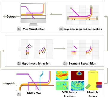
The model for Bayesian mapping followed the workflow depicted in

connection. The datasets consisted of both qualitative (raw images from MTU sensor device, statutory records (utility maps)) as well as quanti-tative information (manhole surveys providing information on

directions and depths). More details are given inSection 2.1.2(MTU

sensor raw data). The data from these sources were integrated together in the form of positions (x,y), depths (z) and orientations (Ɵ) as an

Fig. 1.Model Workflow (Data preprocessing for hypotheses extraction following segment recognition, Bayesian segment connection and refined map visualization.

input for segment recognition algorithm. The geometrical measure-ments (i.e., readings of slope distances in horizontal and vertical planes) with respect to spatial survey structure were acquired using the Total Station Theodolite (TST). The relative positions of the MTU mobile lab-oratory were, therefore, called the survey lines at given (x,y) coordi-nates from the TST. Manhole surveys were helpful in determining the types of buried utilities at a site and estimating their orientations and depths. Bayesian recursive algorithm as known as EM was developed

for segment-manhole connection. EM is an iterative algorithm forfi

nd-ing the maximum-likelihood estimation of a set of parameters for a

spe-cific distribution in a statistical model when it contains unobserved

latent variables (Do and Batzoglou, 2008). Based on partially connected information from different sources and segments recognized from

segment recognition, EM algorithm was used to identify most probable connections of segments with assets and connect them in an iterative manner. The depth information from manholes and sensor readings

were then used in conjunction with EM output to produce re_fined 2D/

3D maps of an investigated site.

2.1. Data preprocessing

Data for model development were collected from following sources;

2.1.1. Statutory records

The utility/statutory records consisted of maps of buried assets as ground truth which provided information on approximate orientations

Fig. 3. (a)MTU scan lines on the surface to record reflections w.r.t. surface excitation and reference measurement location.(b)Correlated functions to create raw images using frequency domain transformation, and(c)hypotheses extracted from raw images using adaptive image segmentation techniques, and integrated with utility records for segment recognition algorithm.

and positions of these assets. Since these records are inaccurate, their position information was not included in segment recognition algo-rithm. However, the information pertaining to the type of buried asset and their approximate directions was helpful in segment-asset connection algorithm. Therefore, the positions and orientations (x,y,

Ɵ)T_{from these records were used for segment-manhole connection}

establishment.

2.1.2. MTU sensor raw data

The raw data included heatmaps (Fig. 2) of investigated sites that were produced from various MTU and commercial sensors. The sensors used in MTU mobile apparatus include Ground Penetrating Radar (GPR), Passive Magnetic Field (PMF), Vibro Acoustic, and Low Frequen-cy Electro-Magnetic (LFEM). Briefly, the sensors and their functionality

are explained in this section. Detailed information on each sensor can be

found elsewhere (Dutta et al., 2013;Muggleton et al., 2011;Thomas

et al., 2009).

2.1.2.1. Ground penetrating radar (GPR).GPR locates buried utilities (me-tallic and non-me(me-tallic) by transmitting electromagnetic waves into the

ground and collecting the response (waves reflected from the objects

underground) (Ristićet al., 2017;Al-Nuaimy et al., 2000). A GPR scan

produces an image as a collection of multiple A-scans of reflected

waves received at different wave-travel times and integrating them into a B-scan. In B-scan, the rows represent depth (by utilizing the

reflected waves) and columns represent horizontal positions of scan

lines.

Fig. 5.Separation of hypotheses into cluster of linear clusters and curved clusters. For clusters with circular features, a three-point circlefitting was used, as inFig. A-1(Appendix).

2.1.2.2. Passive magneticfield (PMF).PMF is useful for detecting the ca-bles by utilizing the magnetic_field generated by current in a cable as

well as neighboring objects which generate magneticfield (may also

be from currentflow leak from a buried cable). The cluster centroids

(Fig. 2c) are multiplied by the surveyed map dimensions (m × n

image) which are then divided by surveyed lengths and depths, respec-tively, to calculate the (x,y,z) coordinates on the map.

2.1.2.3. Vibro acoustic (VA) sensors.VA device at the MTU uses seven geo-phones for recording the reflected velocities of the waves that are gen-erated by exciting the surface. The response received at the surface is utilized to create a cross-sectional image with respect to the reference measurement used near the exciting location. The cross-sectional image is created via the time-domain transformation of the correlation functions between geophone and reference measurement recordings (Figs. 2d,3). The images are then analyzed to extract hypotheses using

adaptive image segmentation techniques (Section 2.1.4, Hypotheses

extraction).

2.1.2.4. Low frequency electromagneticfield (LFEM).LFEM approach is based on injecting the current into the ground and measuring the volt-age on the surface via coupled plates moved along the surface. The LFEM approach at MTU is operated in a targeted grid location and the resulting image represents the underground structure.

Using the above approaches, qualitative raw images consisting of(x,

y,z)T_{information (x-axis as the length of scan line and y-axis as the}

depth of the investigated surface (typically 2–4 m deep)) were collected and processed to extract hypotheses which were utilized for 2D/3D map reconstruction. The orientation of MTU sensor device provides approx-imate direction of buried asset as the survey is usually taken in the di-rection perpendicular to the orientation of asset.

2.1.3. Manhole survey

Manhole surveys for real sites were conducted to collect supporting information on estimated orientations and depths of buried assets. In addition, the types of buried assets were also recorded to distinguish be-tween them when constructing site maps. The quantitative information from manhole surveys therefore included (x,y,z,Ɵ)T_{as well as the type}

of buried asset as qualitative information.

2.1.4. Hypotheses extraction

Hypotheses (processed coordinates of the location detected by MTU sensors) extraction was implemented on raw sensor image data to au-tomatically estimate the positions from surveyed locations. The images were segmented into clusters of foreground (hypotheses) and back-ground pixels using unsupervised image segmentation techniques. The adaptive image segmentation was used to highlight and quantify

Table 1

Settings for simulated and real sites (S# = simulated site #, R# = real site #).

Data # Manholes # Pipes & cables # Sensor readings

S1 10 13 28

S2 12 16 30

S3 26 46 87

R1 19 8 18

R2 8 12 25

•

•

•

•

•

•

regions of high thresholds in the image (NobuyukiOtsu, 1979). Images were initially enhanced based on histogram equalization in order to in-crease image contrast (Krishna, 2013;Gonzalez, 2008). Subsequently,

the adaptive segmentation algorithm (NobuyukiOtsu, 1979), which

regards an image as a data clustering scenario, was applied to divide the image into clusters of two classes (foreground and background)

which iterativelyfinds the threshold that minimizes the weighted

within-class variance and thus, maximizing the between-class variance. The centroids of clusters were identified as approximate positions of

as-sets (e.g.,Fig. 2(b and d)and their backgrounds subtracted (Fig. 2

(right))). Sensor output image is often noisy and may not provide an ac-curate location. Additionally, multiple hypotheses locations may be re-ported in close proximity when different types of assets (or a non-asset object) are present as given inFig. 1(hypotheses extraction). It is noted that the sensory scan lines may consist of multiple hypotheses of different types or a single hypothesis given the ground truth (i.e., utility map inFig. 1). Accordingly, the image segmentation algo-rithm provides clusters (regions) of possibly one or more locations given (i) the type of buried material from utility map, and (ii) raw im-ages provided by different MTU sensor. From multiple imim-ages of a single surveyed location, the most probable locations of assets were estimated using Bayesian weighted average technique, i.e.

h xð Þi ≈N xð;μ;ΛÞ ð1Þ

In the above equation,xidenotes the relative location of hypothesisi

(w.r.t. MTU scan line) collected from the image,μis the mean of selected

hypotheses, andΛis covariance matrix of the hypotheses. Maximum A

Posteriori (MAP) position of an asset was obtained usinghðxÞ ¼ arg

maxΠn

i¼1ðhðxiÞÞwherenis the number of hypotheses.

Prior to segment recognition from groups of hypotheses, the

identi-fication of noise was conducted in terms of points with no manhole

con-nection within a given previously tested threshold (_δ= 2 m). Each

hypothesis point was validated using: (1) point to line (nearest buried utility in statutory record) distance and (2) manhole orientations. The distancedjh(Fig. 3c top right) from each pipe segmentjto the pointh

(Fig. 2d (white circle,Fig. 3b) was calculated using

djh¼

xje−xjs

yjs−yh

− xjs−xh

yje−yjs

ffiffiffiffiffiffiffiffiffiffiffiffiffiffiffiffiffiffiffiffiffiffiffiffiffiffiffiffiffiffiffiffiffiffiffiffiffiffiffiffiffiffiffiffiffiffiffiffiffiffi

xje−xjs

2

þ yje−yjs

2

r ð2Þ

where (xjs,yjs) and (xje,yje) are the start and end points of the pipe seg-mentjrespectively, and (xh,yh) is the location of hypothesis point. The

pointhwas considered an orphan point if its distance from a pipe

segmentjwas greater thanδ. i.e.h¼ orphan if dhk1Nδand dhk2Nδ

hr otherwise

wheredh,skanddh,ekare the distances between ofkmanhole (with

posi-tion (xk, yk), where the segment of same type exists (i.e., a pipe

connection matching pipe segmentjin this case)) from the segment

start and segment end, respectively. The probability that the pointh

be-longs to a segmentjwas then calculated asSj¼ arg max

j ðPhjÞwhere

Phj=F(h→j|djh)≈N(h,djh.)

2.2. Segment recognition

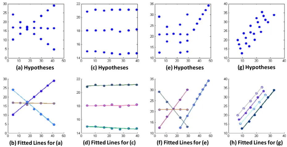
The hypotheses obtained from above step were given as input to seg-ment recognition algorithm which estimated the segseg-ments by joining hy-potheses together based on their positions and orientations. The input to segment identification algorithm included the hypotheses and the orien-tations in which the surveys were taken (usually from left-to-right). The linear segments were iteratively classified from the groups of hypotheses

which were located within the range of an angle of up toε= ± 0.08

(i.e., wider sensitivity of up to 4.5 degrees). The algorithm starts with

first two chosen hypotheses as assigned tofirst class (starts with class = 1), and the orientation from thefirst hypothesis to all other hypotheses are calculated. The next point is chosen and assigned to the same class if

their difference in orientations is≤ εotherwise the chosen point is

assigned a new class. The algorithm is repeated for each hypothesis and provides the output as points assigned to a class which are then joined

using least squares, circle and/or polynomialfitting techniques. The

workflow of the algorithm is given inAlgorithm 1.

Algorithm 1.Segment recognition algorithm (Pseudo code).

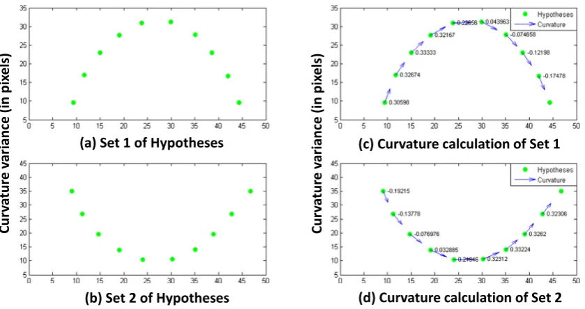
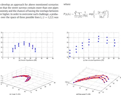
To separate the clusters of linear segments from curved segments, the goodness offit (R2_{) was checked and compared to thresholdε}

1≥0.99

(0.99 confidence). Each cluster withR2≥0.99was separated as a linear pipe segment and the remaining clusters were considered as curved or circular segments. For each hypothesis point in curvature analysis, the tip of the vectorr(t)=bx(t),y(t)Ntraces out a path in the plane wheretrepresented MTU survey line andyrepresented the change in po-sitions represented by hypotheses. The relative popo-sitions of the hypothe-ses points were therefore represented as followsr′(t)=bx′(t),y′(t)N wherex0ðtÞ ¼∂x

∂tandy0ðtÞ ¼∂ y

∂t. The unit tangent vector was calculated asT¼ r0_ðtÞ

kr0_ðtÞk, wherekr0ðtÞk ¼

ffiffiffiffiffiffiffiffiffiffiffiffiffiffiffiffiffiffiffiffiffiffiffiffiffiffiffiffiffiffi

x0_ðtÞ2_þy0ðtÞ2 q

. In order to determine the variation in the position (y) with respect to (x), the difference interval

was obtained usingη¼ k arg max

i∈N ð

TiÞ− arg min i∈N ð

TiÞk. Testing data

clus-ters of various curvatures led to the selection of approximate curvature threshold to 0.15. The segments were assigned as curved using

Curved¼_falsetrue ifðT∈ −½ R;þRorT∈_Otherwise½þR;−RÞand Curvature¼1 ð3Þ

whereCurvature¼ 1_{0 Otherwise}ifη≥0:15

andRis the quantitative measure of

the change iny(Fig. 4).

The curvature detection algorithm was tested on various groups of hypotheses which demonstrated robust performance in terms of

separating curved segments from linear ones (four of the groups given inFig. 5)

2.3. Segment-manhole connection using expectation maximization algorithm

The connection of segments recognized from previous section

with manholes was categorized as a classification problem where

each segment was to be classified as a segment connected to two

manholes. The EM algorithm was proposed for segment-manhole connection establishment which has been used in wide range of

ma-chine learning and data mining scenarios such as classification

(Klautau, 2003;Sander et al., 1998), Image Processing (Huanhuan Chen, 2010) and unsupervised clustering (Bailey and Elkan, 1994;

Buntine, 2002;Salojarvi et al., 2005). The inputs from sensor read-ings, estimated asset orientations from manholes, statutory records and segments recognized from previous step were used to identify suitable connections between segments and manholes. Combining the inputs created a data fusion scenario where hidden information from different sources was integrated and the probability of segment

classification was updated until the algorithm converged (or the

number of iterations reaches). Therefore, based on the probability distribution drawn from EM algorithm, the local maximum of segment-manhole connection provided an optimal solution that was then compared with prior information from statutory records. Using EM, each segment can be assigned to a pair of manhole

Fig. 10.Real Site 1. Blue lines represent simulated utility record based on manhole and sensor readings. Red lines represent segment-manhole connections established by the model. (For interpretation of the references to color in thisfigure legend, the reader is referred to the web version of this article.)

connections given the above parameters. EM consists of two steps that are (1) Expectation and (2) Maximization. Expectation calcu-lates the probability distribution of a target outcome given a set of parameters while the maximization step updates the distribution given the parameters which are updated from expectation at each it-eration. The EM algorithm is explained as follows:

1) For a given hypothesis pointh, get nearest segmentSjfrom statutory

record. Get manhole locations and the depths. Initialise the prior for each manhole connection withPias uniform distribution. Initialise covariance matrix

Λ¼ diagΔd;θj−θk;kθk−θhkk;θj−θhk;kZh−Zkk

whereΔd¼ ffiffiffiffiffiffiffiffiffiffiffiffiffiffiffiffiffiffiffiffiffiffiffiffiffiffiffiffiffiffiffiffiffiffiffiffiffiffiffiffiffiffiffiffiffiffiffiðxSj−xkÞ2þ ðySj−ykÞ 2 q

,θj= orientation ofSj,θk=

ori-entation of segment of same type as ofSjfrom manholek'scover,

θhk= orientation from manhole k to h, zh= depth of h from

sensor,zk= depth of the segment of same type as ofSjfrom manhole

k'scover,Θ= (K,X,Y,Z,xh,yh,zh,Sj)TforKmanholes with [X,Y,Z] as position and depth.

2) E-step: Likelihood for each manholekconnection

L Ch kjΛ;Θi ¼ 1 2πj jΛ

ð Þ3=2 exp −

1 2 C hð ;kÞ

T

Λ−1

C hð ;kÞ

whereC(h,k) = [Δd,‖θj−θk‖,‖θk−θhk‖,‖θj−θhk‖,‖zh−zk‖]. The

Maxi-mum Likelihood Estimate (MLE) is then given byγk¼

LhCkjΛ;Θi

XK

k¼1

LhCkjΛ;Θi

3) M-Step: Maximization of likelihood

Λ¼ diag

ffiffiffiffiffiffiffiffiffiffiffiffiffiffiffiffiffiffiffiffiffiffiffiffiffiffiffiffiffiffiffiffiffiffiffiffiffiffiffiffiffiffiffiffiffiffiffiffiffiffiffiffiffiffiffiffi

∑

k

YK

k¼1

Δd:L Ch kjΛ;Θi

ð Þ

!2

Xk

k¼1

L Ch kjΛ;Θi

v u u u u u u u u t ; ffiffiffiffiffiffiffiffiffiffiffiffiffiffiffiffiffiffiffiffiffiffiffiffiffiffiffiffiffiffiffiffiffiffiffiffiffiffiffiffiffiffiffiffiffiffiffiffiffiffiffiffiffiffiffiffiffiffiffiffiffiffiffiffiffiffiffiffi ∑ k YK

k¼1

θj−θk

_:L Ch kjΛ;Θi

!2

Xk

k¼1

L Ch kjΛ;Θi

v u u u u u u u u t ; ffiffiffiffiffiffiffiffiffiffiffiffiffiffiffiffiffiffiffiffiffiffiffiffiffiffiffiffiffiffiffiffiffiffiffiffiffiffiffiffiffiffiffiffiffiffiffiffiffiffiffiffiffiffiffiffiffiffiffiffiffiffiffiffiffiffiffiffiffi ∑ k YK

k¼1

θk−θhk k k:L Ch kjΛ;Θi

ð Þ

!2

Xk

k¼1

L Ch kjΛ;Θi

v u u u u u u u u t ; ffiffiffiffiffiffiffiffiffiffiffiffiffiffiffiffiffiffiffiffiffiffiffiffiffiffiffiffiffiffiffiffiffiffiffiffiffiffiffiffiffiffiffiffiffiffiffiffiffiffiffiffiffiffiffiffiffiffiffiffiffiffiffiffiffiffiffiffiffiffiffiffi ∑ k YK

k¼1

θj−θhk

_:L Ch kjΛ;Θi

!2

Xk

k¼1

L Ch kjΛ;Θi ; v u u u u u u u u t

zh−zk

k k 0 B B B B B B B B B B B B B B B B B B @ 1 C C C C C C C C C C C C C C C C C C A

4) Repeat 2–3 until converged (log likelihood converges to 10−4₎

5) Maximum A Posteriori (MAP) for connection ofkwithSjisCh→k¼

arg max k∈K ðγkÞ

The MLEγkin step 2 provides best match between a manholekand a

segmentSj. The algorithm is repeated for connection from both ends ofSj

to a pair of best matching manholes. At the test site, it is possible for sen-sors to contain noise (containing spatial location and direction error) as part of the hypotheses. A pointhwas considered noise when it's

likeli-hood of manhole connections (k→andk←) fell below a thresholdα¼

∑h∈OPðLjh;k→;k←Þ 3 2O

whereP(L|h,k→,k←)≈N(L,h,σo). Here,σo(=0.4) is the

variance (meters) calculated from (x,y,z) ofO. The noise from above set of hypotheses points was identified using

h¼ noise if P L hð j ;k→;k←Þbα

h otherwise

ð4Þ

The clusters of segments for manhole connections from (4) consisted of the hypotheses points and the connected manhole positions which are:Cj= [k→ {h∈O:h→Sj} k←]

3. Results and discussion

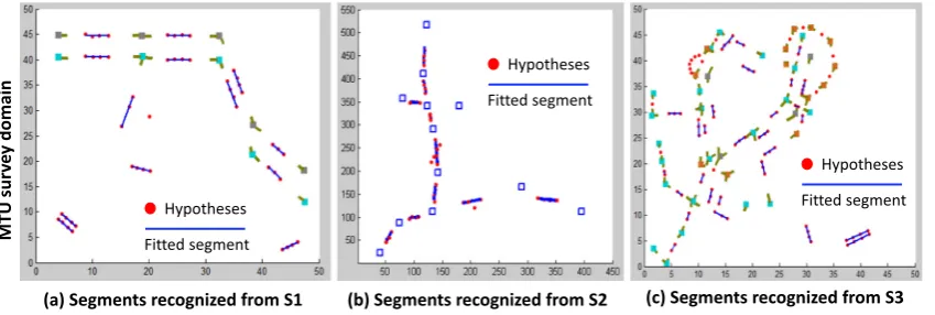
Dataset for model validation includedfive sites of simulated data (3 sets) as well as real data (2 sets). The model was developed and validated using MATLAB 2011(b) where the most probable maps were generated given 3 different sources of information: (i) sensor readings, (ii) manhole surveys, and (iii) the statutory records. In order to validate the model, hy-potheses extraction, accurate segment identification (with noise remov-al) and segment-manhole connection were tested. Several variations in the parameters and data quality were considered in order to verify the ro-bustness of the model. The hypotheses were extracted from raw sensor images using image segmentation techniques. A segment recognition al-gorithm was developed to identify linear and curved pipe/cable segments based on the direction of survey taken by MTU machine, and orientations estimated from hypotheses when they were combined together. Total of 4 initial use cases of hypotheses (Fig. 6) tested in order to evaluate the performance of segment recognition algorithm where the number of seg-ments in each use case were known.

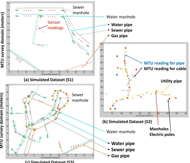
The simulated datasets (S1, S2, and S3) consisted of locations of

manholes as well as pipes from ArcGIS (Esri, 2015) and simulated

hypotheses (simulated readings from MTU sensors). The real sites (R1 and R2) consisted of measurements from MTU sensor readings and statutory records. For noise removal in simulated sets, white noise was added with the following: (1) Spatial noise of the locations of manholes and pipes was up to 2 × 2 m, (2) Noise in hypotheses lo-cations was up to 0.4 m and (3) Noise in pipe directions was up to 8 degrees.

3.1. Bayesian mapping model for simulated data

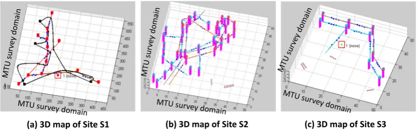
The model was initially tested on 3 simulated datasets (S1, S2 and S3) with varying numbers of manholes, sensor data points, and seg-ments from statutory records (Table 1). For simulated datasets, the hy-potheses were manually generated and the initial maps were obtained from ArcGIS (Esri, 2015). Initial simulated datasets with initial maps are depicted inFig. 7.

(a) Segment recognition: Segment recognition algorithm showed robust performance for all datasets and the noise was removed from groups of hypotheses in S1 and S2. The absence of statutory records did not

affect the capability of the model to draw accurate segments due to the segment recognition algorithm. In addition, the segments were drawn in 3D due to the inclusion of depth information from man-holes and sensor readings. However, the uncertainty increased in the absence of statutory records as they provided useful information on the number of buried assets and their directions. The segments drawn by automated segment recognition algorithm for simulated datasets are given inFig. 8.

(b) Segment-manhole connection: The segment recognition algorithm provided advantages over (Chen and Cohn, 2011) in terms of basis for accurate connection with manholes and construction of 3D maps. The segments were used by EM algorithm for segment-manhole connection establishment. Using the parameters from dif-ferent sources (Materials and Methods), it was observed that the al-gorithm successfully created connections for segments that led to the reconstruction of 3D map. Among the segments generated from step (a) a few segments had single end connecting to a man-hole. Such situations were also tested for the validation of EM algo-rithm. The maps of simulated datasets were generated which are depicted inFig. 9.

3.2. Bayesian mapping model for real data

Real sites (R1and R2) with sensor readings and manhole surveys

were tested for model validation.Table 1provides information on the

inputs to model for simulated sites as well as real sites. There were 18

sensor readings taken at R1which included readings for linear pipes

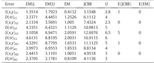
Table 2

Directional(D(Ѳ)), Spatial(S(x,y))and connection errors compared to JCBB.EM\L= without segment recognition algorithm,EM\U= without utility records.

Error EM\L EM\U EM JCBB U E(JCBB) E(EM)

S(x,y)S1 1.3514 1.7923 0.4132 3.1548 2.8 1 0

D(Ѳ)S1 3.3371 4.4451 1.2526 6.1112 4

S(x,y)S2 2.1334 3.5691 1.005 7.4324 2.5 0 0

D(Ѳ)S2 4.3351 6.4321 1.1129 10.9813 5

S(x,y)S3 3.1058 6.9471 2.0591 12.6976 6.5 5 0

D(Ѳ)S3 4.6131 8.8195 2.0031 16.9115 6

S(x,y)R1 4.3291 8.7795 1.6531 11.1125 5 1 0

D(Ѳ)R1 3.9973 6.9553 1.8533 8.8134 4

S(x,y)R2 2.4415 3.1101 1.0051 4.9518 3 0 0

and an electricity cable. Raw images from sensors were manipulated to extract hypotheses which were used for automatic segment

recognition. There were no connection errors for R1using EM based

segment-manhole connection algorithm for linear segments (See

Fig. 10).

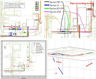
Real site R2consisted of straight linear pipes with an electric cable

for which the sensor readings were taken (Fig. 11a). There was no

noise detected in the sensor readings and segments were successfully connected with manholes. PMF sensor usually detects objects with elec-trical current such as electric cables. At R2, The PMF sensor detected a

water pipe (rectangle inFig. 11b) in the survey. This was due to the

run of an electric cable in a close proximity of that water pipe which emits the electrical current.

3.3. Connection and spatial errors in mapping models

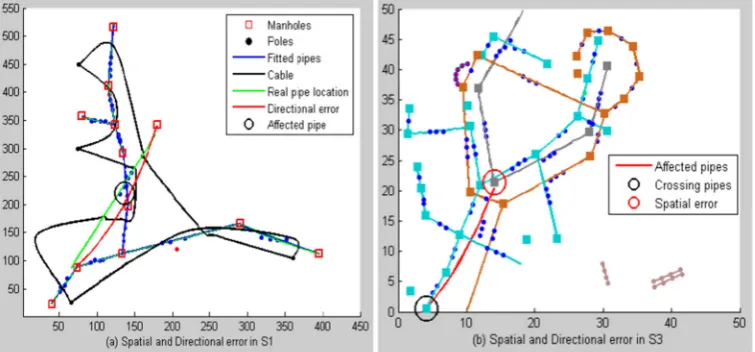
For manhole connection establishment process, the proposed algo-rithm was also compared with Joint Compatibility Branch & Bound (JCBB) which calculates the Mahalanobis distance between the observa-tions and the predicobserva-tions and accepts a connection if the Mahalanobis distance is smaller than a validation gate (Yangming Li et al., 2013). The segment-manhole connection problem was similar to the spatial

data association problem in robotics (Bailey and Durrant-Whyte,

2006). Using the data fusion technique, noise removal and the iterative

refinement of posterior probability using EM algorithm, the analysis

showed better results compared to JCBB for both simulated sets as well as real sites. JCBB suffered in connecting segments in simulated sce-narios with manholes when more than one segments were located in close proximity in the map. In tested datasets, JCBB also suffered from connection errors at the manhole locations where directional error

exceededfive degrees. There were totalfive manhole connection errors

recorded when JCBB was run on S3 as shown inFig. 12whereFig. 12a

shows the connection errors for water pipes andFig. 12b shows the con-nection errors for gas pipes.

The analysis with segment recognition algorithm significantly

re-duced the spatial errors (in meters) and directional errors (in de-grees) when modeling for mapping the underground utilities. The mean directional error using EM algorithm was smaller compared to JCBB. The connection errors (i.e., false positives (number of man-holes connections predicted for the wrong segment)) are given in

Table 2which are denoted as E(JCBB) for JCBB and E(EM) for EM algorithm.

A noticeable impact on the voxel prediction for each pipe was ob-served when this error rate was increased from 8 to 14 degrees. The

in-creased directional error in S1 and S3 had significant effect with

inaccurate segment-manhole connections in the maps. In addition, the spatial error resulted in variations in voxel classification as shown in

Fig. 13a and b. The black circles show directional errors and the red cir-cles show spatial error.

4. Conclusions

The traditional approaches for map generation given in the literature require information from statutory records and provide solutions for mostly 2D map generation. Additionally, the information from multiple sensors require extensive processing and statutory records should also be integrated that provide prior knowledge about buried utilities. Re-cent analyses/studies on the abilities to locate underground utilities stressed the needs of a system capable of generating real time maps with the help of heterogeneous information. However, current tech-niques are limited to either generating 2D maps of linear segments or unable to detect different types of utilities. This paper addresses these problems by proposing a Bayesian mapping model by implementing various machine learning techniques for real time 3D map (re)construc-tion. The segment recognition algorithm is robust in identifying groups of hypotheses forming linear/curved segments that are helpful in estab-lishing connections with manholes. In order to improve utility classifi

-cation and refined map generation, noise removal facilities were

embedded in the system that improved performance in distinguishing between hypotheses and noise. The Bayesian Mapping model is aimed to overcome critical issues related to efficient and real-time location of buried assets that could provide valuable underground information and be cost effective. Further online analysis will also validate model

performance at higher levels and its ability to generate refined maps

at real time.

Contributions

The research and development activities were conducted mainly at the University of Leeds, under the supervision of Professor Antho-ny G. Cohn. First author conducted the analysis, prepared results and the manuscript under the supervision of Prof. Anthony Cohn, second author conducted major revisions and improvements in the paper, while other authors at partner institutions contributed to the

development of MTU sensors and providing raw data from Wigan and Blagdon test sites.

Conflicts of interest

The authors do not have any con_flict of interest.

Acknowledgements

This research is supported by EPSRC grants (EP/F06585X/1 and EP/ K021699/1): Mapping the Underworld: Multisensory Device Creation,

Assessment, Protocols (http://www.mappingtheunderworld.ac.uk).

We are thankful to the project management, especially, Mark Hamilton, for all site visits, collaboration and management of the efforts from all project partners.

Appendix A. Appendix

For curved segments, the three-point circle_fitting was applied as il-lustrated inFig. A-1.

A. Most probable segment estimation

In order to refine the output of linear segmentfitting without

sig-nificant impact on model performance, the least squaresfitting was

performed on the above sets of hypotheses and manhole connec-tions. Even though the data from multiple sources was integrated for Bayesian mapping, the sensor readings may contain small non-negligible noise which may also affect the performance of least

squares linearfitting algorithm.Fig. A-2shows a simple scenario

where the point containing noise in its location causes an increased angular difference with the orientation from connecting manhole.

Also, the segment approximation fails tofind the most probable

linear segment without crossing any other segment in close proximity.

It is critical to develop an approach for above mentioned scenarios since it is common that the street surveys contain more than one pipes buried in close proximity and the chances of having the overlaps between those segments are higher. In order to overcome such challenge, a proba-bility distribution over the space of three possible linesLi(i = 1,2,3) was

created and described by discrete random variables.Liis theith_{line of}

voxels given the specific attributes which are the locations of the points of clusters de_fined in previous section. We need to_find

arg max l

Ygl

l¼1

P yðljL1;L2;L3Þ

ð Þ ðA1Þ

and

arg max l

Ygl

l¼1

P zðljL1;L2;L3Þ

ð Þ ðA2Þ

wherel∈glis the voxel chosen from a setglof voxelsfitted for the

quantized line. The probability distribution for three observed possible

3D positions of each lineLiwere created and combined givenx,yand

zinformation. For each voxel of a lineLi, two equal spaced perpendicular line segmentsℊpwere drawn along the y-axis for Eq.(A1)and z-axis for

Eq.(A2). This set of linear segments is denoted byG. For the calculation of the most probable voxel at each quantised position of each lineLi, we use two terminologies. For Eq.(A1), the pixelpil_{ofLiis the (xl,yl) and for}

Eq.(A2), the pixelpilofLiis the (yl,zl). Therefore Eq.(A1)is used for

de-termining the most probableyth_{position of the voxel and Eq.(A2)is}

used to determine thezth_{position of the voxel in the map. For allk}

voxels de_fined bygl, the joint probability distributions are given by

P yðljL1;L2;L3Þ ¼ YL

i¼1

P yð ljLiÞfor L¼3

P zðljL1;L2;L3Þ ¼ YL

i¼1

P zðljLiÞfor L¼3

where

P yðljLiÞ ¼ Xgl

l¼1 X

y∈G

1 ∇y

k k exp −

y−pl i

2

gp 2

( )

ðA3Þ

pil_{is thel}th_{pixel (xl,yl) ofLi}

P zðljLiÞ ¼ Xgl

l¼1 X

z∈G

1 ∇z

k k exp −

z−pl i

2

gp 2

( )

ðA4Þ

pil_{is thel}th_{pixel (yl,zl) ofLi}

CalculatingP(yl|Li) andP(zl|Li) provide the probabilitiesP(yl|L1,L2,L3) andP(zl|L1,L2,L3) respectively which are used to calculate the most prob-able voxel position for the map using

P L yjL1;L2;L3¼ arg max l

Ygl

l¼1

P yð ljL1;L2;L3Þ

ð Þ ðA5Þ

and

P Lð zjL1;L2;L3Þ ¼ arg max l

Ygl

l¼1

P zðljL1;L2;L3Þ

ð Þ ðA6Þ

An example of this is shown in Fig. A-3 where three lines

(L1,L2,L3) are drawn from three techniques and the quantized

lines on y-axis and z-axis are drawn to calculate Eqs.(A5) and

(A6).

At each step in the map, the voxel with the highest probability given three lines as input was taken as the most probable voxel. The set of all voxels at the end created a line in 3D space which was considered as the most probable linear segment approximation. This algorithm was ap-plied for the approximation of each linear segment in the performance evaluation of the algorithm.

B. Cardinal splinefitting

In addition to the linear and curved pipe segments which may include sewer pipes, gas pipes and water pipes, the street maps also included electric cables buried underground which need to be approximated. The difference of the cables from the other pipe segments is their non-linear behavior. The cable can be buried in an arbitrary order without satisfying linearity condition for

which linefitting or curve approximation may represent

inappro-priate solutions. The Passive Magnetic Field (PMF) sensors report the sequence of the survey locations when performing street

sur-vey. Forfitting cables and non-linear segment, Cardinal Spline

al-gorithm was implemented which was capable forfitting the lines

to points in both 2D and 3D. The detailed explanation of Cardinal

Spline algorithm is provided elsewhere (Ali Khan and Sarfraz,

2011).

C. Probabilistic voxel classification

Errors in the linearity of segment lines vary depending on the noise added in sensor and manhole readings. In addition, the presence of multiple closely-buried assets is challenging when rec-ognizing the number of segments. In order to address these chal-lenges, linear approximation algorithm was useful as it integrated information from multiple sources and provided most probable esti-mation of voxel classification. Bayesian probabilistic voxel classifi

ca-tion showed improved results in terms offitted lines when compared

to least squaresfitting.

Fig. A-3.Perpendicular quantised linear points created from the point and the linear segment.

References

Aleardi, M., Ciabarri, F., Mazzotti, A., 2017. Probabilistic estimation of reservoir properties by means of wide-angle AVA inversion and a petrophysical reformulation of the Zoeppritz equations. J. Appl. Geophys. 147 (Supplement C):28–41 Available at:.

http://www.sciencedirect.com/science/article/pii/S0926985117301192.

Ali Khan, M., Sarfraz, M., 2011.Motion tweening for skeletal animation by cardinal spline. In: Abd Manaf, A., Sahibuddin, S., Ahmad, R., Mohd Daud, S., El-Qawasmeh, E. (Eds.), Informatics Engineering and Information Science. Springer, Berlin Heidelberg.

Al-Nuaimy, W., et al., 2000. Automatic detection of buried utilities and solid objects with GPR using neural networks and pattern recognition. J. Appl. Geophys. 43 (2):157–165 Available at.http://www.sciencedirect.com/science/article/pii/S0926985199000555. Ashdown 2000. Mains Location Equipment–A State of the Art Review and Future

Re-search Needs. In: UKWIR (Ed.). (ISBN: 1 84057 233 7).

Bailey, T., Durrant-Whyte, H., 2006.Simultaneous localization and mapping (SLAM): part II. IEEE Robotics & Automation Magazine 13 (3), 108–117.

Bailey, T.L., Elkan, C., 1994.Fitting a mixture model by expectation maximization to dis-cover motifs in biopolymers. Proceedings International Conference on Intelligent Sys-tems for Molecular Biology. 2, pp. 28–36.

Bar-Shalom, Y., 1987.Tracking and Data Association. Academic Press Professional, Inc., San Diego, CA, USA.

Bhalerao, Abhir, Wilson, R., 2001.A Fourier Approach to 3D Local Feature Estimation from Volume Data (2001). British Machine Vision Conference. pp. 461–470.

Buntine, W., 2002.Variational Extensions to EM and Multinomial PCA. In: Elomaa, T., Mannila, H., Toivonen, H. (Eds.), Machine Learning: ECML 2002. Springer Berlin Heidelberg.

Burtwell, M., E. A., 2004.Locating underground plant and equipment - proposals for a re-search programme. UKWIR (ISBN: 1-84057).

Chen, Huanhuan, A. G. C, 2010.Probabilistic robust hyperbola mixture model for interpreting ground penetrating radar data. The 2010 International Joint Conference on Neural Networks (IJCNN). IEEE, Barcelona.

Chen, H., Cohn, A.G., 2011. Buried utility pipeline mapping based on multiple spatial data sources: A Bayesian data fusion approach. IJCAI Retrieved from.https://doi.org/ 10.5591/978-1-57735-516-8/IJCAI11-402.

Chen, T.W., Wang, Q., 2010. 3D line segment detection algorithm for large-scale scenes. 2010 International Conference on Audio, Language and Image Processing: pp. 1056–1061https://doi.org/10.1109/ICALIP.2010.5685113.

Christensen, C.W., et al., 2015. Combining airborne electromagnetic and geotechnical data for automated depth to bedrock tracking. J. Appl. Geophys. 119 (Supplement C):178–191 Available at:.http://www.sciencedirect.com/science/article/pii/S0926985115001585. Delicado, P., Smrekar, M., 2007. Mixture of nonlinear models: a Bayesianfit for principal

curves. 2007 International Joint Conference on Neural Networks:pp. 195–200

https://doi.org/10.1109/IJCNN.2007.4370954.

Dettmer, J., et al., 2014. Trans-dimensionalfinite-fault inversion. Geophys. J. Int. 199 (2): 735–751 Available at.https://doi.org/10.1093/gji/ggu280.

Do, C.B., Batzoglou, S., 2008. What is the expectation maximization algorithm? Nat. Biotechnol. 26:897.https://doi.org/10.1038/nbt1406.

Dong-Min, W., Dong-Chul, P., 2009.3D line segment detection based on disparity data of area-based stereo. Intelligent systems, 2009. GCIS '09. WRI Global Congress on, 19–21 May 2009, pp. 219–223.

Dutta, R., Cohn, A.G., Muggleton, J.M., 2013. 3D mapping of buried underworld infrastruc-ture using dynamic Bayesian network based multi-sensory image data fusion. J. Appl. Geophys. 92:8–19 Available at:.http://www.sciencedirect.com/science/article/pii/ S0926985113000311.

Esri, 2015. Put Your Maps to Work with ArcGIS, the Mapping Platform for Your Organiza-tion [Online]. Esri Available:.https://www.arcgis.com.

Ester, M., Kriegel, H.-P., Sander, J., Xu, X., 1996.A density-based algorithm for discovering clusters a density-based algorithm for discovering clusters in large spatial databases

with noise. Proceedings of the Second International Conference on Knowledge Dis-covery and Data Mining. AAAI Press, pp. 226–231.

Fernández-Martínez, J.L., et al., 2013.From Bayes to Tarantola: new insights to under-stand uncertainty in inverse problems. J. Appl. Geophys. 98 (Supplement C), 62–72.

Fiannacca, P., et al., 2017.IG-Mapper: A new ArcGIS® toolbox for the geostatistics-based automated geochemical mapping of igneous rocks. Chem. Geol. 470 (Supplement C), 75–92.

Friedman, J., Popescu, B., 2004.Gradient Directed Regularization for Linear Regression and Classification (Retrieved from citeulike-article-id:3142778).

Gonzalez, R.C., 2008.Digital Image Processing. Third Ed.

Guo, R., et al., 2011.Non-linearity in Bayesian 1-D magnetotelluric inversion. Geophys. J. Int. 185 (2), 663–675.

Ji, Y., et al., 2016.Frequency-domain sparse Bayesian learning inversion of AVA data for elastic parameters reflectivities. J. Appl. Geophys. 133 (Supplement C), 1–8.

Klautau, Aldebaro, N. J. A. A. O, 2003.Discriminative Gaussian mixture models: a compar-ison with Kernel classifiers. In: Mishra, T.F.A.N. (Ed.), Proceedings of the 20th Interna-tional Conference on Machine Learning (ICML-03).

Krishna, A.S., Rao, G.S., 2013.Contrast enhancement techniques using histogram equaliza-tion methods on color images with poor lightning. Int. J. Comput. Sci. Eng. Appl. 15–24.

Mcmahon, W., Burtwell, M.H., Evans, M., 2005.Minimising street works disruption: the real costs of street works to the utility industry and society. UKWIR.

Muggleton, J.M., Brennan, M.J., Gao, Y., 2011.Determining the location of buried plastic water pipes from measurements of ground surface vibration. J. Appl. Geophys. 75 (1), 54–61.

Neira, J., Tardos, J.D., 2001.Data association in stochastic mapping using the joint compat-ibility test. IEEE Trans. Robot. Autom. 890–897.

Oldenborger, G.A., et al., 2016.Bedrock mapping of buried valley networks using seismic reflection and airborne electromagnetic data. Journal of Applied Geophysics 128 (Supplement C), 191–201.

Otsu, Nobuyuki, 1979.A threshold selection method from gray-level histograms. IEEE Trans. Syst. Man Cybern, SMC-9 62–66.

Ren, H., et al., 2017.Bayesian inversion of seismic and electromagnetic data for marine gas reservoir characterization using multi-chain Markov chain Monte Carlo sampling. J. Appl. Geophys. 147 (Supplement C), 68–80.

Ristić, A., et al., 2017.Point coordinates extraction from localized hyperbolic reflections in GPR data. J. Appl. Geophys. 144 (Supplement C), 1–17.

Royal Acd, R. C., Atkins Pr, Brennan Mj, Chapman Dn, Chen H, Cohn Ag, Curioni G, Foo Ky, Goddard K, Hao T, Lewin Pl, Metje N, Muggleton Jm, Naji A, Pennock Sr, Redfern Ma, Saul Aj, Swingler Sg and Wang P 2010. Mapping the Underworld: Lo-cation, Mapping and Positioning Without Excavation. In: Control, C. (Ed.). (Mid-dle East, Singapore).

Royal, A.C.D., Atkins, P.R., Brennan, M.J., Chapman, D.N., Chen, H., Cohn, A.G., Foo, K.Y., Goddard, K.F., Hayes, R., Hao, T., Lewin, P.L., Metje, N., Muggleton, J.M., Naji, A., Orlando, G., Pennock, S.R., Redfern, M.A., Saul, A.J., Swingler, S.G., Wang, P., Rogers, C.D.F., 2011.Site assessment of multiple-sensor approaches for buried utility detec-tion. Int. J. Geophys. 2011, 19.

Salojarvi, J., Puolamaki, K., Kaski, S., 2005.Expectation maximization algorithms for condi-tional likelihoods. Proceedings of the 22nd Internacondi-tional Conference on Machine Learning. ACM, Bonn, Germany.

Sander, J., Ester, M., Kriegel, H.-P., Xu, X., 1998.Density-based clustering in spatial data-bases: the algorithm GDBSCAN and its applications. Data Min. Knowl. Discov. 2, 169–194.

Sanquer, M., Chatelain, F., El-Guedri, M., Martin, N., 2011.A reversible jump MCMC algo-rithm for Bayesian curvefitting by using smooth transition regression models. Acous-tics, Speech and Signal Processing (ICASSP). 2011 IEEE International Conference on, 22–27 May 2011, pp. 3960–3963.

Thomas, A.M., et al., 2009.Stakeholder needs for ground penetrating radar utility location. J. Appl. Geophys. 67 (4), 345–351.

Underworld, M.T., 2011. Mapping the Underworld [Online]. Available:. http:// www.mappingtheunderworld.ac.uk, Accessed date: 13 September 2015.

Wang, Y., Lu, W., 2016.Discontinuity enhancement based on time-variant seismic image deblurring. J. Appl. Geophys. 135 (Supplement C), 155–162.

Ward, G., Hastie, T., Barry, S., Elith, J., Leathwick, J.R., 2009. Presence-only data and the em al-gorithm. Biometrics 65 (2):554–563.https://doi.org/10.1111/j.1541-0420.2008.01116.x.

Werman, M., Keren, D., 1999.A novel Bayesian method forfitting parametric and non-parametric models to noisy data. Computer Vision and Pattern Recognition, 1999. IEEE Computer Society Conference on 1999 Vol. 2, pp. 1–558.