Covariance Estimation from Limited Data: State-of-the-Art, Algorithm Implementation, and Application to Wireless Communications

Theses

12-2018

Covariance Estimation from Limited Data:

State-of-the-Art, Algorithm Implementation, and

Application to Wireless Communications

Ian Tomeo

[email protected]

Follow this and additional works at:https://scholarworks.rit.edu/theses

This Thesis is brought to you for free and open access by RIT Scholar Works. It has been accepted for inclusion in Theses by an authorized administrator of RIT Scholar Works. For more information, please [email protected].

Recommended Citation

Communications

By

Ian Tomeo

A Thesis Submitted

in

Partial Fulfillment

of the

Requirements for the Degree of

MASTER OF SCIENCE

in

Electrical Engineering

Approved by:

PROF

(Dr. Panos P. Markopoulos, Research Advisor)

PROF

(Dr. Sohail A. Dianat, Department Head)

PROF

(Dr. Andres Kwasinski., Committee Member)

PROF

(Dr. Sohail A. Dianat, Committee Member)

DEPARTMENT OF ELECTRICAL AND MICROELECTRONIC ENGINEERING

KATE GLEASON COLLEGE OF ENGINEERING

ROCHESTER INSTITUTE OF TECHNOLOGY

ROCHESTER, NEW YORK

A

BSTRACT

Acknowledgements

I would sincerely like to thank Panos Markopoulos for his aid in the creation of this thesis and for giving me the chance to work with him in this field. I would also like to thank those in the SCAN research group at RIT that have helped me to pursue this opportu-nity. “I don’t know half of you half as well as I should like; and I like less than half of you half as well as you deserve.” — Tolkien

Contents

Acknowledgements ii

List of Figures vi

List of Tables ix

List of Abbreviations x

List of Symbols xii

1 Introduction 1

1.1 Covariance Matricies . . . 1

1.2 System Model . . . 2

1.3 Standard Filtering Options . . . 3

1.4 Reduced Rank Filters . . . 4

2 Auxillary Vector Filtering 6 2.1 AV Algorithm . . . 6

2.2 Selection of Termination Index . . . 6

2.3 Numerical Studies . . . 9

2.4 Results . . . 9

2.4.1 Post-Filtering SINR and BER vs N . . . 9

2.4.2 Post-Filtering SINR and BER vs SNR . . . 11

2.4.3 Post-Filtering SINR and BER vs K . . . 12

2.4.4 Post-Filtering SINR and BER vs INR . . . 14

2.4.5 Post-Filtering SINR and BER vs D . . . 15

2.4.6 PDF vs Estimation Error . . . 17

3 Eigenvalue Fixing Filtering 18 3.1 Benefits of EIF Filter . . . 18

3.2 Proposed Eigenvalue Fixing Method . . . 18

3.3 Selection ofα . . . 19

3.3.1 Kth Eigenvalue . . . 19

3.3.2 J-Divergence . . . 20

3.4 Numerical Studies . . . 20

3.5 Results . . . 20

3.5.2 Post-Filtering SINR and BER vs SNR . . . 22

3.5.3 Post-Filtering SINR and BER vs Number of Sig-nals . . . 24

3.5.4 Post-Filtering SINR and BER vs INR . . . 25

3.5.5 Post-Filtering SINR and BER vs D . . . 27

3.5.6 Eigenvalues vs Index . . . 28

4 Diagonal Loading Estimation 30 4.1 Reason for Diagonal Loading . . . 30

4.2 Ledoit-Wolf Shrinkage Estimate . . . 30

4.3 Rao-Blackwell Ledoit-Wolf Shrinkage Estimate . . . 32

4.4 Oracle Shrinkage Estimate . . . 32

4.5 OAS Shrinkage Estimate . . . 33

5 Probability Based Estimation 34 5.1 Probabilistic Approach . . . 34

5.2 Diagonally Loaded Empirical Bayes . . . 35

5.3 Haff’s Empirical Bayes . . . 35

5.4 Regularized Partial Covariance Estimation . . . 36

6 Minimax Estimates 38 6.1 A Minimum Loss Estimate . . . 38

6.2 Stein Minimax Estimate . . . 38

6.3 Improved Minimax Estimate . . . 39

6.4 LWd Estimate . . . 39

6.5 Stein-Haff Estimate . . . 40

6.6 QuEST Estimate . . . 42

7 Structured Estimates 44 7.1 Shaped Estimates . . . 44

7.2 Banding Estimate . . . 44

7.3 Thresholding Estimate . . . 45

7.4 POET Estimate . . . 46

8 Hybrid Estimates 48 8.1 Estimates of Multiple Types . . . 48

8.2 NERCOME Estimate . . . 48

8.3 Integrated Estimate . . . 49

8.4 LOOC . . . 51

8.5 RDA . . . 54

9 Numerical Studies 55 9.1 Comparison of Covariance Performance . . . 55

9.3 Diagonal Loading Filtering . . . 58

9.4 Probability Based Filtering . . . 59

9.5 Minimax Filtering . . . 61

9.6 Structured Filtering . . . 63

9.7 Hybrid Filtering . . . 65

9.8 Average BER . . . 67

9.9 Classification . . . 71

10 Conclusions 72 10.1 What Type of Filter to Use . . . 72

10.2 Filter Performance . . . 72

List of Figures

2.1 The AV filter generates a sequence of vectors that pro-duces the final filter wieghts, first proposed in Pados and Karystinos, 2001. . . 7 2.2 A termination index for the AV filter is determined by

the proposed JMOV technique. . . 8 2.3 Post-Filtering SINR [dB] vs N with SNR= −8 [dB],

K = 5, INR= 8[dB] per interfering source,D= 40. . . . 10 2.4 BER vsNwith channel estimated from half of the

snap-shots and BER calculated with remaining snapsnap-shots, SNR= −8 [dB], K = 5, INR= 8 [dB] per interfering source,D= 40. . . 10 2.5 Post-Filtering SINR [dB] vs SNR [dB] with N = 50,

K = 5, INR= 8[dB] per interfering source,D= 40. . . . 11 2.6 BER vs SNR [dB] with channel estimated from half

of the snapshots and BER calculated with remaining snapshots, N = 50, K = 5, INR= 8 [dB] per interfer-ing source,D= 40. . . 12 2.7 Post-Filtering SINR [dB] vsK withN = 50, SNR=−8

[dB], INR= 8[dB] per interfering source,D= 40. . . 13 2.8 BER vsKwith channel estimated from half of the

snap-shots and BER calculated with remaining snapsnap-shots,

N = 50, SNR= −8[dB], INR= 8[dB] per interfering source,D= 40. . . 13 2.9 Post-Filtering SINR [dB] vs INR [dB] with N = 50,

SNR=−8[dB],K = 5,D= 40. . . 14 2.10 BER vs INR [dB] with channel estimated from half

of the snapshots and BER calculated with remaining snapshots,N = 50, SNR=−8[dB],K = 5,D= 40. . . . 15 2.11 Post-Filtering SINR [dB] vsDwith N = 50, SNR=−8

[dB],K = 5, INR= 8[dB] per interfering source. . . 16 2.12 BER vsDwith channel estimated from half of the

snap-shots and BER calculated with remaining snapsnap-shots,

2.13 Post-Filtering SINR [dB] vs termination index (0-5000) with N = 50, SNR=−8[dB],K = 5, INR= 8[dB] per interfering source,D= 40. . . 17

3.1 Post-Filtering SINR [dB] vs N with SNR= −10 [dB],

K = 5, INR= 5[dB] per interfering source,D= 40. . . . 21 3.2 BER vsNwith channel estimated from half of the

snap-shots and BER calculated with remaining snapsnap-shots, SNR= −10[dB], K = 5, INR= 5 [dB] per interfering source,D= 40. . . 22 3.3 Post-Filtering SINR [dB] vs SNR [dB] with N = 50,

K = 5, INR= 5[dB] per interfering source,D= 40. . . . 23 3.4 BER vs SNR [dB] with channel estimated from half

of the snapshots and BER calculated with remaining snapshots, N = 50, K = 5, INR= 5 [dB] per interfer-ing source,D= 40. . . 23 3.5 Post-Filtering SINR [dB] vs K with N = 50, SNR=

−10[dB], INR= 5[dB] per interfering source,D= 40. . 24 3.6 BER vsKwith channel estimated from half of the

snap-shots and BER calculated with remaining snapsnap-shots,

N = 50, SNR=−10[dB], INR= 5 [dB] per interfering source,D= 40. . . 25 3.7 Post-Filtering SINR [dB] vs INR [dB] with N = 50,

SNR=−10[dB],K = 5,D= 40. . . 26 3.8 BER vs INR [dB] with channel estimated from half

of the snapshots and BER calculated with remaining snapshots,N = 50, SNR=−10[dB],K = 5,D= 40. . . 26 3.9 Post-Filtering SINR [dB] vsDwithN = 50, SNR=−10

[dB],K = 5, INR= 5[dB] per interfering source. . . 27 3.10 BER vsDwith channel estimated from half of the

snap-shots and BER calculated with remaining snapsnap-shots,

N = 50, SNR= −10 [dB], K = 5, INR= 5 [dB] per interfering source. . . 28 3.11 Eigenvalues vs Index with N = 50, K = 5, INR= 5

[dB] per interfering source,D= 40. . . 29 3.12 Eigenvalues vs Index (Zoomed) withN = 50, K = 5,

INR= 5[dB] per interfering source,D= 40. . . 29

5.1 The Reguralized Partial Complex Gaussian (REGPCG) algorithm attempts to improve upon a starting esti-mate while ignoring outliers . . . 37

9.1 Common Estimation: Post-Filtering SINR [dB] vs SNR [dB] vs INR [dB],N = 50,K = 5,D= 40. . . 57 9.2 SCM Estimation: Post-Filtering SINR [dB] vs SNR [dB]

vs INR [dB],N = 50,K = 5,D= 40. . . 57 9.3 Ledoit-Wolf Estimate: Post-Filtering SINR [dB] vs SNR

[dB] vs INR [dB],N = 50,K = 5,D= 40. . . 58 9.4 Rao-Blackwell Ledoit-Wolf Estimate: Post-Filtering SINR

[dB] vs SNR [dB] vs INR [dB],N = 50,K = 5,D= 40. . 58 9.5 OAS Estimate: Post-Filtering SINR [dB] vs SNR [dB]

vs INR [dB],N = 50,K = 5,D= 40. . . 59 9.6 EB-DL Estimate: Post-Filtering SINR [dB] vs SNR [dB]

vs INR [dB],N = 50,K = 5,D= 40. . . 59 9.7 Haff’s Empirical Baysian Estimate: Post-Filtering SINR

[dB] vs SNR [dB] vs INR [dB],N = 50,K = 5,D= 40. . 60 9.8 Regularized Partial Covariance Estimation: Post-Filtering

SINR [dB] vs SNR [dB] vs INR [dB], N = 50, K = 5,

D = 40. . . 60 9.9 Stein Minimax Estimate: Post-Filtering SINR [dB] vs

SNR [dB] vs INR [dB],N = 50,K = 5,D= 40. . . 61 9.10 Improved Minimax Esimate: Post-Filtering SINR [dB]

vs SNR [dB] vs INR [dB],N = 50,K = 5,D= 40. . . 61 9.11 LWd Esimate: Post-Filtering SINR [dB] vs SNR [dB]

vs INR [dB],N = 50,K = 5,D= 40. . . 62 9.12 Stein-Haff Esimate: Post-Filtering SINR [dB] vs SNR

[dB] vs INR [dB],N = 50,K = 5,D= 40. . . 62 9.13 QuEST Estimate: Post-Filtering SINR [dB] vs SNR [dB]

vs INR [dB],N = 50,K = 5,D= 40. . . 63 9.14 Banding Estimate: Post-Filtering SINR [dB] vs SNR

[dB] vs INR [dB],N = 50,K = 5,D= 40. . . 63 9.15 Thresholding Estimate: Post-Filtering SINR [dB] vs SNR

[dB] vs INR [dB],N = 50,K = 5,D= 40. . . 64 9.16 POET Estimate: Post-Filtering SINR [dB] vs SNR [dB]

vs INR [dB],N = 50,K = 5,D= 40. . . 64 9.17 NERCOME Estimate: Post-Filtering SINR [dB] vs SNR

[dB] vs INR [dB],N = 50,K = 5,D= 40. . . 65 9.18 Integrate Banding Estimate: Post-Filtering SINR [dB]

vs SNR [dB] vs INR [dB],N = 50,K = 5,D= 40. . . 65 9.19 Integrate POET Estimate: Post-Filtering SINR [dB] vs

SNR [dB] vs INR [dB],N = 50,K = 5,D= 40. . . 66 9.20 Integrate Double Estimate: Post-Filtering SINR [dB]

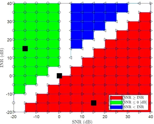
vs SNR [dB] vs INR [dB],N = 50,K = 5,D= 40. . . 66 9.21 Pertinent sections of System Model which are

List of Tables

9.1 The average BER of various covariance matricies when SNR ≥INR from the grid shown in the above figure 9.21. HereN = 50,K = 5, andD= 40 . . . 68 9.2 The average BER of various covariance matricies when

SNR≤0 [dB] from the grid shown in the above figure 9.21. HereN = 50,K = 5, andD= 40 . . . 69 9.3 The average BER of various covariance matricies when

SNR <INR from the grid shown in the above figure 9.21. HereN = 50,K = 5, andD= 40 . . . 70 9.4 The classification accuracy of common classification

List of Abbreviations

AV AuxiliaryVector

AWGN AdditiveWhiteGaussianNoise

BER BitErrorRate

CCM CommonCovarianceMatrix

CV-MOV CrossValidated-MinimumOutputVariance

DL DiagonalLoading

EB EmpiricalBayes

EBH Haff’sEmpiricalBayes

EIF EIgenvalueFixing

GE GeneralizedEigenvalues

INR Interference toNoiseRatio

IM ImprovedMinimax

JMOV JDivergence and the inverse CV-MOV KL Kullback-Leibler Divergence

LOOC LeaveOneOutCovariance Estimate

LOOL LeaveOneOutLikelihood

LS LeastSquares

LW LedoitWolf

MF MatchedFilter

ML MaximumLikelihood

MMSE Minimum-Mean-Square-Error

MSE MeanSquaredError

MVDR Minimum-Variance-DistortionlessResponse

NERCOME NonparametricEigenvalue-Regularized Precision or

COvarianceMatrixEstimator

OAS Oracle’sShrinkage

PC PrincipalComplement

PCA PrincipleComponentAnalysis

PDF ProbabilityDensityFunctions

POET PrincipalOrthogonal complEmentThresholding

PSK PhaseShiftKeying

QuEST QuantizedEigenvaluesSamplingTransform

RBLW RaoBlackwellLedoitWolf

RDA RegularizedDiscriminantAnalysis

REGPCG REGuralizedPartialCovariamceGuassian Estimation

ample ovariance atrix

SIMO SingleInputMultipleOutput

SINR Signal toInterference-plus-NoiseRatio

SL Stein’sLoss

SM Stein’sMinimax

SMI Sample-Matrix-Inversion

SNR Signal toNoiseRatio

List of Symbols

D Number of receive (base-station) antennas

N Number of snapshots

K Number of signals (user + interferers)

Ps Signal power PI Interferance power

H Channel matrix with perfect channel knowledge h Channel of signal of interest

y Received-signal vector

Y DbyN matrix of received snapshots

bi ith bit of signal of interest

ii ith interference vector created from interfering signals n Noise vector

σ2 _{Variance of the AWGN present at the receiver}

E Transmitted Energy

Σ Covariance matrix of random vectorY Q Matrix of ordered eigenvectors

qi theith eigenvector

Λ Matrix of ordered eigenvalues

λi theith eigenvalue

w Weighting vector for antenna array I Identity matrix

0 Vector of zeros

d AV algorithm termination index

α EIF fixing value

ρ DL shrinkage coefficient F DL shrinkage target

µ mean of covariance matrix Ψ Wishart parameter matrix

ν Wishart degrees of freedom

γ Measure of how much one trusts the prior estimate

β_REGPCG The order of partial estimation Φ Matrix of altered eigenvalues

φi Theith altered eigenvalue

Word Matrix and vector of weights for LWd estimate

F Spectral sample distribution

i,j Array element within 1 Index Function

R Risk

k Banding and Thresholding parameter

M Number of sample splits

ψ Current sample split

si,j(.) Generalized shrinkage function τi,j Entry-adaptive threshold n Class

m Split location of the samples

M Number times split samples are averaged

Chapter 1

Introduction

1.1

Covariance Matricies

The proliferation of internet enabled devices has caused our commu-nication infrastructure to becoime congested. Many of the 5G com-munication systems are experiencing more interference generated by themselves and outside sources. Current communication standards require the use of large antenna arrays in order to estimate a signal of interest Honig and Golstein, 2002; Nadakuditi and Edelman, 2008. Large arrays are important for quickly communicating substantial amounts of information over massive distances.

The standard method to estimate the weighting which should be applied to each array element is known as Sample Matrix Inver-sion (SMI) Carlson, 1988. SMI is known to attain low performance when experiencing the case of limited training data. In forming a co-variance matrix estimate we want the number of training samplesN

to be significantly greater than the sampled array size D. When the number of samples available for filter estimation is low with respect to the filter length (i.e., the size of the array), estimation with an in-terference suppressive filter becomes a challenging problem. When there is not a large enough data set to come close to estimating the true covariance matrix, this is known as "small-sample-support," and it constitutes the practical application scenario when the array size is very large and the environment reasonably varying across time –the case becomes even more pronounced when the environment changes fast, e.g., in urban setups. In this case the duration of the coherence interval does not allow for the collection of enough samples for the array’s high dimensionality.

Lamare and Sampaio-Neto, 2007, and maximum likelihood covari-ance estimation filters Abrahamsson, Selen, and Stoica, 2007; Culan and Adnet, 2016; Coluccia, 2015. Arguably, one of the most suc-cessful methods for interference suppression under "small-sample-support" is auxiliary-vector (AV) filtering Pados and Karystinos, 2001.

Novel contributions of this thesis will include choosing an im-proved termination index for Auxiliary Vector (AV) filtering which can be found in Chapter 2. Introduction of Eigenvalue Fixing (EIF) filtering produces better results than reduced rank filtering in Chap-ter 3. These improved filChap-ters show significant reduction of error rate than the current standards. The performance of the aforementioned filters and other filters is analyzed when utilizing modern covariance matrix estimates by varying parameters of the system model to de-termine what the best filter and covariance estimate to use would for any given situation found in Chapter 9.

1.2

System Model

At this point it will be of benefit to review the construction of a co-variance matrix. We will assume a random vector y of length D is drawn from a random distribution. y =

y1· · ·yD

T

. From this we may determine the mean vector of the distribution, this vector gives insight of the class of the distribution which may vary in either in variance or in the mean vector. the mean vector represents the av-erage value for each of the individual D dimensions in the sample space. µ = E[y]. Where µis the mean vector of random vector y. The covariance matrix is a matrix whose element in the i,j position is the covariance between theith andjth elements of a random vec-tor. Σ=E[(y−E[y])(y−E[y])T]. WhereΣis the Covariance matrix of random vectory.

Many adaptive filtering problems want to solve a problem of the form w = Σ−1h in order to obtain a weighting vectorw. Con-sider the scenario of a base-station with very a large number of anten-nas that needs to apply max-Signal to Interferance plus Noise Ratio (SINR) and Minimum Mean Squared Error (MMSE) filtering for in-terference suppression. We consider a single-input multiple-output (SIMO) uplink system where the source transmit symbols from some complex alphabet A in the presence of colored complex Gaussian disturbance. The transmitted signal is collected by the reciever with an array of length D. The i-th down-converted and pulse-matched received-signal vector is of the form

where bi is thei-th communicated symbol, transmitted with energy E = _E{|bi|2}, ii is a random complex, zero-mean Gaussian

interfer-ence vector with autocorrelation ΣI, and ni is the additive white

Gaussian noise (AWGN) vector, distributed by CN (0D, σ2ID),

in-dependently of bi and ii. The receiver applies filter w and detects ˆ

bi = Q(wHyi), whereQ(·)is a thresholding function pertinent to the

symbol alphabet A (e.g., for A = {±1}, Q(·) = sgn<{·}). Ideally, wHyi is exactly equal to bi at the receiver. Practically, the receiver

will minimize the mean squared error (MSE)J(w) =_E{|bi−wHyi|2},

using the standard MMSE filterw_MMSE =Σ−1_{h, where}

Σ=E{yyH}=E{hhH}+ΣI+σ2ID (1.2)

as shown in Trees, Bell, and Tian, 2013. It is known thatw_MMSE also maximizes the post-filtering SINR.

We calculate the Post-Filtering SINR as

SIN R= DPs<{|wh H_|2_}

w(ΣI+σ2I)wH

. (1.3)

Whereσ2_{is the variance of the AWGN present at the receiver, andP}

s

is the power of the signal of interest. In this paper for simplicity we will use the same recieved interference power PI for each interferer

so our interferance covariance matrix will be

ΣI =DPIHHH. (1.4)

WhereHis the matrix composed of interference channels.

1.3

Standard Filtering Options

If interference from other signals is do not have large power content a lot of the time the best filter to use is the matched filter. This filter just sets the weights of the filter to the estimate of the channel

wMATCHED = ˆh. (1.5)

ˆ

hin (1.5) can be previously known, or estimated as

ˆ

h= 1

N_pYpbp (1.6)

where b_p ∈ ANp is a vector of pilot symbols carried inYp, such that Yp = [yp1,yp2, . . .ypN]and yp corresponds with bp. In subsequent

matched filter can be improved upon using a good covariance matrix estimate.

In practice,Σis unknown and commonly estimated by the sam-ple covariance matrix (SCM) obtained by samsam-ple-averaging Pourah-madi, 2013

ˆ

ΣSCM=

1 NYY

H

. (1.7)

where snapshot matrix Y = [y1,y2, . . .yN]. Assumes N chorent

re-cieved signal vectors that follow the model of (1.1). WhenY_pis also used for the estimates ofΣˆSCM in (1.7), then the Least-Squares filter

w_LS = (Y_pYH

p) −1_Y

pbp is formed Lee, Morf, and Friedlander, 1981.

Using estimate (1.7), the receiver can estimatew_MMSEby the standard sample-matrix inversion (SMI) filter Trees, 2002

w_SMI= ˆΣ−_SCM1 hˆ. (1.8) This will set the filter weights to values that will null undesired in-terference. Σˆ_SCM and w_SMI together are known to perform poorly whenN is short, with respect to the array dimensionalityD–even if

N is greater thanD andΣˆSCM is invertible. When dimensionality is

greater than the number of samples SCM becomes singular and the SMI fails. The SCM also has an over dispersed variance when operat-ing with "small-sample-support." We can no longer use conventional estimation techniques due to the limited number of samples while there are a large number of features available. A method to increase output performance of the filter is to use a better conditioned covari-ance matrix estimate.

When the available number of coherent snapshots that will be used for filter estimation is “not large enough” with respect to the ar-ray dimensionality due to the large numbers of receiver element and interference signals we must rely on other estimation methods. Some common methods used to estimate the MMSE filter are the Singular-Value-Decomposition (SVD) Reduced Rank (RR) filter Honig and Golstein, 2002, Krylov filter Lamare and Sampaio-Neto, 2007, and the Auxiliary Vector (AV) filter Pados and Karystinos, 2001; Qian and Batalama, 2003.

1.4

Reduced Rank Filters

SINR. For RR filters the number of signals present in a system K

must be known to estimate the filter weights. Modern techniques have been developed using analysis of the Wishart distribution to estimate the number of signals that a receiver sees Nadakuditi and Edelman, 2008. These techniques are not ideal when the number of available samples is small compared to the number of signal sources and the issue is exacerbated when sample vectors have very large di-mensions. When using reduced rank filtering the filter will not use eigenvectors and eigenvalues that contain low power.

In the case of Strobach, 1996 rank reduction will act upon the principle eigenvalues of the system’s covariance matrix. To use this filter SVD must be performed on the SCM,

ˆ

ΣSCM=

YYH

N =QΛQ H

. (1.9)

Where Λ is the matrix whose diagonal entries contain the ordered set of eigenvalues which means that the eigenvalues are placed in descending order (λ1 > λ2 > ... > λD ) Dey and Srinivasan, 1985;

Takemura, 1984 andQis the matrix created from the corresponding eigenvectors. Inversion of the SCM under systemic interference is improved upon in SVD reduced rank filtering where we will con-sider the inversion of Λ on the subspace containing of the first K

eigenvalues to be close enough. If Q¯ and Λ¯ represent the matrices containing the firstK ordered eigenvectors and eigenvalues respec-tivley then we have

w_SVD = ¯QΛ¯−1Q¯Hhˆ ≈Σˆ−_SCM1 hˆ. (1.10) If the number of pertinent signal sources is unknown this reduced rank filter requires the use of estimation techniques forKas in Nadaku-diti and Edelman, 2008.

Unlike SVD rank reduction Krylov filters Honig and Golstein, 2002 use instead

w_KRLV =Q_KRLV(QH_KRLVΣˆ_SCMQ_KRLV)−1QH_KRLVhˆ (1.11) with,

Chapter 2

Auxillary Vector Filtering

2.1

AV Algorithm

Auxiliary-vector filtering, introduced in Pados and Karystinos, 2001; Batalama, Medley, and Pados, 2000 is an iterative algorithm that initializes filter wieghts to the matched filter and, operating on the standard SCM, converges to the SMI filter Karystinos et al., 2008; Markopoulos, Kundu, and Pados, 2013. Most importantly, prior to convergence, AV that is carried out without matrix memory deliv-ers a sequence of filtdeliv-ers that attain superior SINR performance than SMI. This is particuarly pronounced in "small-sample-support." Thus the need to identify a preferred termination index for the AV to dis-play good SINR performance is a point of significance in the AV lit-erature. Two approaches, cross-validation and J-divergence, have been proposed in Qian and Batalama, 2003. Because AV iterations converge to SMI without any explicit matrix inversion it makes AV particularly appealing for applications where the array size is very large. Matrix inversion being cubic with respect to the autocorre-lations matrix size Strassen, 1969, together with its superior "small-sample-support" performance, arguably render AV a preferred filter for interference suppression in large arrays. Based upon the previ-ous relizations, AV filtering seems to be emerging as a preferred ap-proach Sklivanitis et al., 2018. We seek to further improve the perfor-mance of AV by proposing a new criterion for AV iteration termina-tion that is at least as accurate as current methods which can show improvement when experiencing moderate levels of interference.

2.2

Selection of Termination Index

We now steer our focus onto the selection of a termination index

d, so that wd exhibits high SINR and low-MSE. In Qian and

Algorithm 1: AV Algorithm

Input: Σˆ,h,wH_{h= 1,d}

MAX

Output: w0,w1,w2, . . . ,wdMAX

1: w0 = khhk

2: ford= 1tod_MAX

3: gd = ˆΣwd−1− ˆ

hhˆH

khˆk2Σwˆ d−1

4: ifgd=0

5: exit

6: ζd=

gH dΣwˆ d−1

gH dΣgˆ d

7: wd=wd−1−ζdgd

8: return w0,w1,w2, . . . ,wdMAX

FIGURE2.1: The AV filter generates a sequence of vec-tors that produces the final filter wieghts, first

pro-posed in Pados and Karystinos, 2001.

validated minimum output variance (CV-MOV) estimation and J-Divergence estimation. CV-MOV estimation attempts to minimize the filtered output noise and interference and is defined as

ˆ

dCV-MOV= min

d

( _N X

i=1

wH_d/iyiyHi wd/i

)

. (2.1)

We observe that the CV-MOV method does not perform optimally when the estimate of the channel is not ideal and performance is not optimum in a high SNR setting. The weights analyzed when using CV-MOV should not be normalized or otherwise scaled after being generated from Algorithm 1 as this can bias the minimum output variance. The J-Divergence estimate leverages the SNR of received samples and is defined as

ˆ

dJ-Div = max

d

(

4[_N1 PN

i=1mi] 2 1

N PN

i=1m2i −[N1

PN

i=1mi]2

)

(2.2)

mi =|<{wHd yi}|. (2.3)

Algorithm 2: JMOV Algorithm

Input: Y,hˆ,dMAX

Output: d_JMOV

Initialization:

1: Σˆ1 =Covariance Estimate (Y)

2: [w_J0,wJ1,. . .,wJdMAX] =AV Algorithm( ˆΣ1,hˆ, dMAX)

3: fori= 1toN

4: Σˆ2 =Covariance Estimate (Y/i)

5: [w_MOV0/i,wMOV1/i,. . .,wMOVdMAX/i] =AV( ˆΣ2,hˆ, dMAX)

6: LMAX=−inf 7: ford= 1tod_MAX

8: c1 = 0,c2 = 0,c3 = 0

9: fori= 1toN

10: mi =|<{w_JHdYi}|

11: c1 ←c1+mi/N

12: c2 ←c2+m2i/N

13: c3 ←c3+w_MOVH _d/iYiYiHwMOVd/i

14: L=

4c2₁ c₂−c2

1 c3

15: ifLMAX> L

16: LMAX←L

17: d_JMOV ←d

18: return dJMOV

FIGURE 2.2: A termination index for the AV filter is determined by the proposed JMOV technique.

be shown that the JMOV estimate will provide close to if not the best estimation in any given system. The criterion are combined such that the J-Divergence and the inverse CV-MOV (JMOV) are maximized. The JMOV estimation method is

ˆ

dJMOV = max

d     

4[_N1 PN i=1mi]2

1

N

PN i=1m2i−[

1

N PN

i=1mi]2 PN

i=1w

H d/iyiy

H i wd/i

     . (2.4)

2.3

Numerical Studies

All interference channels are uniformly distributed between 80 de-grees and 100 dede-grees out of phase with the channel of the signal of interest. In the model used for numerical studies interference power experienced at the receiver is equal for all interference sources. Simu-lations in this chapter are repeated 5000 times for each plot and a new realization of signal channels is generated each repetition. When generating the figures the channel of the signal of interest is esti-mated with half of the snapshots used as pilot snapshots and the BER is calculated from the remaining snapshots. The maximum number of AVs generated isdMAX= 500.

2.4

Results

2.4.1

Post-Filtering SINR and BER vs N

FIGURE2.3: Post-Filtering SINR [dB] vsNwith SNR=

−8[dB], K = 5, INR= 8 [dB] per interfering source,

D= 40.

FIGURE 2.4: BER vs N with channel estimated from half of the snapshots and BER calculated with remain-ing snapshots, SNR=−8[dB],K = 5, INR= 8[dB] per

2.4.2

Post-Filtering SINR and BER vs SNR

In the next numerical study shown in figures 2.5 and 2.6, we fixN = 50,K = 5, INR= 8[dB],D= 40and evaluate the post-filtering SINR for varying SNR. We plot the Post-Filtering SINR vs SNR and BER vs SNR respectively. The J-Divergence is sabotaged when the SNR< 0

[dB] however this has minimal effect upon the JMOV estimate which partially depends on CV-MOV.

FIGURE 2.5: Post-Filtering SINR [dB] vs SNR [dB] with N = 50, K = 5, INR= 8 [dB] per interfering

FIGURE2.6: BER vs SNR [dB] with channel estimated from half of the snapshots and BER calculated with re-maining snapshots, N = 50,K = 5, INR= 8[dB] per

interfering source,D= 40.

2.4.3

Post-Filtering SINR and BER vs K

Next in Fig. 2.7 and Fig. 2.8, we fix SNR=−8[dB],N = 50, INR= 8

FIGURE 2.7: Post-Filtering SINR [dB] vsK withN = 50, SNR=−8[dB], INR= 8[dB] per interfering source,

D= 40.

FIGURE 2.8: BER vs K with channel estimated from half of the snapshots and BER calculated with remain-ing snapshots, N = 50, SNR= −8[dB], INR= 8[dB]

2.4.4

Post-Filtering SINR and BER vs INR

Then in Fig. 2.9 and Fig. 2.10, we fix SNR=−8[dB],N = 50.,K = 5,

D = 40and vary the INR. We plot SINR vs INR in Fig. 2.9 and BER vs INR in Fig. 2.10. The figures show using JMOV offers the best performance. It is of note that at the extreme of almost no interfer-ence power J-Diverginterfer-ence performs very well and CV-MOV becomes a better estimator than J-Divergence as the INR increases. This plot shows that relative performance of JMOV is minimally affected by INR.

FIGURE2.9: Post-Filtering SINR [dB] vs INR [dB] with

FIGURE2.10: BER vs INR [dB] with channel estimated from half of the snapshots and BER calculated with re-maining snapshots, N = 50, SNR= −8 [dB],K = 5,

D= 40.

2.4.5

Post-Filtering SINR and BER vs D

FIGURE2.11: Post-Filtering SINR [dB] vsDwithN = 50, SNR=−8[dB],K = 5, INR= 8[dB] per interfering

source.

FIGURE 2.12: BER vsDwith channel estimated from half of the snapshots and BER calculated with remain-ing snapshots,N = 50, SNR=−8[dB],K = 5, INR= 8

2.4.6

PDF vs Estimation Error

In Fig. 2.13 the Probability Density Functions (PDFs) are plotted of the index estimation errorein estimated termination indices dˆfrom the ideal Oracle termination indexdO withe= ˆd−dO. CV-MOV has

the largest spread for error centered around -5 followed by the much tighter hybrid JMOV technique centered at -1 and has the smallest total estimation error, the J-Divergence estimation has a very tight spread centered 0.

This experiment is run with the maximum number of AVs gen-erateddMAX= 5000and where we fix SNR=−8[dB],N = 50,K = 5,

INR= 8[dB],D= 40.

FIGURE2.13: Post-Filtering SINR [dB] vs termination

Chapter 3

Eigenvalue Fixing Filtering

3.1

Benefits of EIF Filter

A common technique to deal with interference is to use SVD reduced rank filtering. When SNR of the signal of interest is low SVD reduced rank filtering does not attempt to consider the noise power contained in the system which is a large component of the SINR. When the es-timation of the total number of signals present in the system is not correct the reduced rank filter does not operate optimally and one of the signals in the system could be buried in what is considered to be noise. If we fix the eigenvalues to be constant for eigenvectors that are not thought to correspond to pertinent signals, we can at least use the SCM’s eigenvector information that we have already went through the effort of obtaining through SVD. The Eigenvalue Fix-ing (EIF) filterFix-ing method presented here uses the eigenvectors that were not being taken advantage of in SVD reduced rank filtering, This allows for better compensation for AWGN in the system. EIF produces better results than SVD reduced rank filtering alone when SNR is below 0 [dB].The J-Divergence method currently used to es-timate the number of AVs to use in an AV filter is used to improve estimation techniques of the EIF filter. A survey of the use of the EIF filter with different parameter estimation methods is performed varying the system model across various parameters.

3.2

Proposed Eigenvalue Fixing Method

the covariance matrix by using the form as follows:

˜

Λ=

_¯ Λ 0

0 αI

(3.1)

whereαis a constant we have the covariance matrix estimate

ΣEIF=QΛQ˜ H. (3.2)

Begining with normalized covariance matricies we can calculate the MSE of our estimate from the ideal estimate as

M SE =kΣ_MMSE−Σ_EIFk2

(3.3)

=kQ_MMSEΛ_MMSEQH_MMSE−QΛQ˜ Hk2

(3.4)

AssumingQ_MMSE ≈QandΛ¯_MMSE ≈Λ¯ we have

M SE =kQ¯( ¯Λ_MMSE−Λ¯) ¯QH + ¯Q0(βI−αI) ¯Q0Hk2

(3.5)

= (β−α)2kQ¯0Q¯0Hk2_.

(3.6)

Here Q¯0 represents the ordered eigenvectors after the first K. Or-dered eigenvalues after the first K of the MMSE covariance matrix represent the noise Nadakuditi and Edelman, 2008; Strobach, 1996 and are constant, β is the scaled variance of the AWGN present at the receiver. If α is 0 the EIF filter becomes the SVD based reduced rank filter. It is of note for a normalized matrix that as

lim

SNR→∞β = 0 (3.7)

and as

lim

SNR→−∞β=λK. (3.8)

This means as the SNR decreases the value chosen for α will have an important cancellation effect withβin reducing the MSE from the ideal covariance matrix.

3.3

Selection of

α

In order to produce filter weights that will yield a high SINR a good value forαmust be selected.

3.3.1

Kth Eigenvalue

3.3.2

J-Divergence

The J-Divergence criterion derived in Qian and Batalama, 2003, will choose anα that will minimize the error a filter by finding the filter weights that will maximize the difference between symbol interpre-tation of different bits. The criterion is based upon maximizing the Kullback–Leibler divergence of snapshots. The method estimates the value ofαas follows.

ˆ

αJ = max

α

(

4[_N1 PN

i=1mi]2

1

N PN

i=1m2i −[

1

N PN

i=1mi]2

)

(3.9)

with

mi =|<{wHαyi}|. (3.10)

The above blind J-Divergence criterion will pick the value ofαto use relatively close to that of the ideal EIF filter. This technique is much slower than just choosing the Kth eigenvalue as the filter weights need to be calculated multiple times. When the SNR of the signal of interest is at or below 0 [dB], when the amount of interference becomes large, and when the number of snapshots is relatively low the J-Divergence estimate ofαwill degrade.

3.4

Numerical Studies

Simulations have been performed using the aforementioned system model. All interference channels in Hare uniformly distributed be-tween 80 degrees and 100 degrees out of phase with the channel of the signal of interest. Simulations are repeated 5000 times for each plot and a new realization of signal channels is generated each time. For each figure the Krylov filter using the K = 5 for subspace size Lamare and Sampaio-Neto, 2007, and SVD reduced rank filter are shown. The EIF-Kth Eigenvalue filter is usingα = λK. The channel

of the signal of interest is estimated from half of the total snapshots used to generate the covariance matrix.

3.5

Results

3.5.1

Post-Filtering SINR and BER vs N

increases the better the J-Divergence selection criterion performs. Fig 3.2 shows that the BER of the normal EIF filter is nearly ideal across allN.

FIGURE3.1: Post-Filtering SINR [dB] vsNwith SNR=

−10[dB],K = 5, INR= 5[dB] per interfering source,

FIGURE 3.2: BER vs N with channel estimated from half of the snapshots and BER calculated with remain-ing snapshots, SNR= −10[dB], K = 5, INR= 5[dB]

per interfering source,D= 40.

3.5.2

Post-Filtering SINR and BER vs SNR

FIGURE 3.3: Post-Filtering SINR [dB] vs SNR [dB] with N = 50, K = 5, INR= 5 [dB] per interfering

source,D= 40.

FIGURE3.4: BER vs SNR [dB] with channel estimated from half of the snapshots and BER calculated with re-maining snapshots, N = 50,K = 5, INR= 5[dB] per

3.5.3

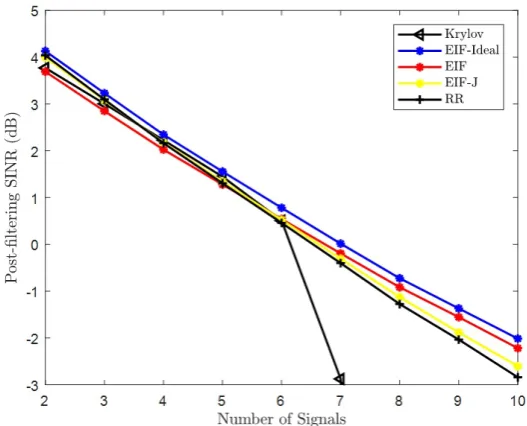
Post-Filtering SINR and BER vs Number of

Sig-nals

Figures 3.5 and 3.6 show that as the number of signals in the sys-tem increases the EIF filter performance increases in comparison to the SVD reduced rank filter. For small numbers of interferers the J-Divergence criterion performs close to the ideal EIF filter.

FIGURE 3.5: Post-Filtering SINR [dB] vsK withN = 50, SNR= −10 [dB], INR= 5 [dB] per interfering

FIGURE 3.6: BER vs K with channel estimated from half of the snapshots and BER calculated with remain-ing snapshots,N = 50, SNR=−10[dB], INR= 5[dB]

per interfering source,D= 40.

3.5.4

Post-Filtering SINR and BER vs INR

FIGURE3.7: Post-Filtering SINR [dB] vs INR [dB] with

N = 50, SNR=−10[dB],K= 5,D= 40.

FIGURE3.8: BER vs INR [dB] with channel estimated from half of the snapshots and BER calculated with re-maining snapshots, N = 50, SNR= −10[dB],K = 5,

3.5.5

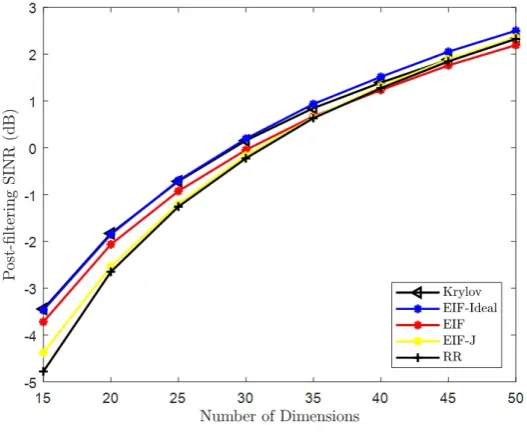
Post-Filtering SINR and BER vs D

Figures 3.9 and 3.10 show that as the number elements in the system decreases the better the EIF filter performs when compared to the Reduced Rank filter. For small numbers of elements the Kth eigen-value method coverges to the ideal EIF filter. For large numbers of elements the J-Divergence criterion converges to the ideal EIF filter.

FIGURE 3.9: Post-Filtering SINR [dB] vsDwith N = 50, SNR= −10 [dB],K = 5, INR= 5[dB] per

FIGURE 3.10: BER vsDwith channel estimated from half of the snapshots and BER calculated with remain-ing snapshots, N = 50, SNR= −10 [dB], K = 5,

INR= 5[dB] per interfering source.

3.5.6

Eigenvalues vs Index

FIGURE3.11: Eigenvalues vs Index withN = 50,K = 5, INR= 5[dB] per interfering source,D= 40.

FIGURE 3.12: Eigenvalues vs Index (Zoomed) with

N = 50, K = 5, INR= 5[dB] per interfering source,

Chapter 4

Diagonal Loading Estimation

4.1

Reason for Diagonal Loading

In previous sections we have explored how to perform filtering by finding ways to set our weights given a sample set, now we turn our attention to methods of improving our covariance matrices that are fed into our different filter types. We must develop estimation techniques to mitigate estimation error under "low sample support". Typically systems will require fast estimation algorithms which the benefit the final estimate more from the computational speed in place of taking more samples. This is why the diagonal loading estimate is commonly used with small N. When we do not have enough sam-ples to create a nonsingular sample covariance matrix we can make our estimate approach a positive definite matrix so we will be able to invert it. A given matrixF, will always be invertable if it consists of only positive diagonal elements with zeros elsewhere. For any real invertible matrix F, the product FT_{Fis a positive definite}

ma-trix. From this result we see that adding Fto any other matrix will cause the final matrix to come closer to being positive definite. Our DL covariance matrix Carlson, 1988; Du, Li, and Stoica, 2010; Ledoit and Wolf, 2004; Chen et al., 2010 will appear as

ˆ

ΣDL = ˆΣSCM+ρF. (4.1)

Where ρ is a shrinkage coefficient and positive definite matrix F is our shrinkage target. Fis commonly the identity matrix and we can find our DL wieghts as

wDL= ( ˆΣSCM+ρI)−1hˆ. (4.2)

4.2

Ledoit-Wolf Shrinkage Estimate

we begin with the intention of minimize the MSE

E[kΣˆ −Σk2_F] (4.3) using the estimator

ˆ

Σ= (1−ρ) ˆˆΣSCM+ ˆρFˆ. (4.4)

Hereρˆis the estimated shrinkage coefficient and the SCM is used as a low bias estimate of the true covariance matrix. Here the shrinkage targetFˆ = T r(ΣSCM)

D Iis a low variance estimate which will correct the

SCM. We derive the optimal Shrinkage coefficient from the MSE. For this we need the following definitions

µ=hΣ,Ii, (4.5)

α2_LW =kΣ−µIk2, (4.6)

β_LW2 =E[kΣ_SCM−Σk2_],

(4.7)

δ_LW2 =E[kΣSCM−µIk2]], (4.8)

α2_LW+β_LW2 =δ2_LW, (4.9) and

min ρ1,ρ2

E[kΣˆ −Σk2

F]s.t.Σˆ =ρ1ΣˆSCM+ρ2I. (4.10)

It can be shown that the MSE can be broken down into our Diagonal Loading form as

E[kΣˆ −Σk2

F] =

α2

LWβLW2

δ2

LW

ˆ

Σ= α

2

LW

δ2

LW

ˆ

Σ_SCM+ β

2

LW

δ2

LW

µI. (4.11)

An estimate is derived for optimal shrinkage by estimating each op-timal parameter as

µ=hΣ,Ii ≈µˆ=hΣˆ_SCM,Ii, (4.12)

β_LW2 =E[kΣˆSCM−Σk2]≈bLWˆ =

1 N2

i=1

kyiyTi −ΣˆSCMk2, (4.14)

b2_LW =min( ˆb_LW2, d2_LW), (4.15) and

α2_LW =kΣ−µIk2 _≈a2

LW =d

2

LW−b

2

LW. (4.16)

The Ledoit-Wolf (LW) Estimator is an estimate of the optimal esti-mate defined as

ˆ

ΣLW =

a2

LW

d2

LW

ˆ

ΣSCM+

b2

LW

d2

LW

ˆ

µI= (1−ρˆLW) ˆΣSCM+ ˆρLWFˆ. (4.17)

The LW shrinkage coefficient is

ˆ ρLW =

PN

i=1kyiyTi −ΣˆSCMk2F

N2_{[T r(( ˆΣ}

SCM)2)− T r

2_{( ˆΣ}

SCM)

D ]

(4.18)

4.3

Rao-Blackwell Ledoit-Wolf Shrinkage

Es-timate

The Rao-Blackwell Ledoit-Wolf (RBLW) Estimator found in Chen et al., 2010 builds upon the LW estimate. Beginning with the LW shrink-age coefficient we evaluate the previous expectations using the Rao-Blackwell Theorem. The Rao-Rao-Blackwell theorem states estimateg(X)

given sufficient statistic T(X) is never worse than estimateg(X)on its own. So If all samples are Gaussian then we can assume LW is Gaussian and the estimate will be improved. The RBLW shrinkage coefficient becomes

ˆ

ρ_RBLW = N−2

N T r(( ˆΣSCM)

2_{) +T r}2_{( ˆΣ}

SCM)

(N + 2)[T r(( ˆΣ_SCM)2₎₋ T r2( ˆΣSCM)

D ]

. (4.19)

4.4

Oracle Shrinkage Estimate

The ideal Diagonal Loading technique is shown in Chen et al., 2010. This is the best result diagonal loading can achieve as an estimator. The idea is again to minimize the MSE,

using estimatorΣˆi. The Oracle Estimator specifies the optimal

shrink-age coefficient for the Gaussian distribution and will be used as a benchmark to see how well algorithms could perform. The optimal shrinkage coefficient for any given distribution is,

ρO =

E[T r((Σ−ΣˆSCM)( ˆF−ΣˆSCM))]

E[kΣˆSCM−Fˆk2_F]

. (4.21)

As one evaluates these expectations under Gaussian assumptions the shrinkage estimator becomes

ρ_O = (1−

2

D)T r(Σ

2_{) +T r}2_(Σ)

(N + 1− 2

D)T r(Σ2) + (1− N

D)T r2(Σ)

. (4.22)

4.5

OAS Shrinkage Estimate

The OAS estimator Chen et al., 2010 uses an iterative approach to estimate the Oracle’s shrinkage coefficient for a normal distribution. The iteration is

ˆ ρj+1 =

(1− 2

D)T r( ˆΣjΣˆSCM) +T r

2_{( ˆΣ}

j)

(N + 1− 2

D)T r( ˆΣjΣˆSCM) + (1− N

D)T r2( ˆΣj)

(4.23)

where the covariance estimate iterates as

ˆ

Σj+1 = (1−ρˆj+1) ˆΣSCM+ ˆρj+1Fˆ. (4.24)

In order to obtain a closed form expression under Gaussian assump-tions we solve for the OAS shrinkage coefficient at convergence to be

ˆ

ρ_OAS = (1−

2

D)T r(( ˆΣSCM)

2_{) +T r}2_{( ˆΣ}

SCM)

(N + 1− 2

D)[T r(( ˆΣSCM)2)− T r2_{( ˆΣ}

SCM)

D ]

(4.25)

In each of these algorithms assumeρˆ∗ = max(min( ˆρ,1),0)and useρˆ∗

Chapter 5

Probability Based Estimation

5.1

Probabilistic Approach

If the random variables of a system follow a known probability dis-tribution one may attempt to correct a covariance matrix by solving a maximum likelihood equation. The most common type of distribu-tion solved is the Wishart distribudistribu-tion which is formed by multivari-ate Guassian random variables. The Wishart Distribution is a gen-eralizedχ2-distribution i.e. W1(σ2, ν) = σ2χ2ν. In Coluccia, 2015 the

covariance matrix is estimated using Empirical Bayes (EB) by find-ing the shrinkage coefficient of estimate as in chapter 4 to optimize diagonal loading. For this technique we consider a zero-mean multi-variate normal vector fory. GivenΣ, the probability of choosing Y is

f(Y|Σ) =

QN

i=1exp[−y

H

i Σ−1yi] πDN_detN_(Σ) =

exp[T r(−Σ−1ΣˆSCM)]

πDN_detN_(Σ) . (5.1)

Assuming the conjugate prior is a Wishart distribution with the pa-rameter matrixΨandνdegrees of freedom makesΣhave an inverse Wishart distribution withN +ν degrees of freedom. The estimate is calculated as

ˆ

ΣEB = (1−ρ) ˆΣSCM+ρFˆ (5.2)

where

ˆ

F= Ψ

ν−D (5.3)

and

ρ= ν−D

N +ν−D. (5.4)

The maximum of the likelihood function of f(Y|Ψ, ν) is calculated to obtain the ML estimate of the parameter matrix

ˆ

The EB estimate utilizing the ML parameter matrix is

ˆ

Σ_EB = (1−ρ) ˆΣ_SCM+ρ ˆ

Ψ

ν−D =

N +ν N+ν−D

ˆ

Σ_SCM. (5.6)

A performance metric for covariance estimation includes the Kullback-Leibler (KL) divergence. KL defined as

KL[ ˆΣ,Σ] = 1 2[T r( ˆΣ

−1_Σ)−D+ln(det( ˆΣ)

det(Σ))] (5.7)

is a measure of dissimilarity between probability distributions. This metric gives an idea of how much the model has yet to learn.

5.2

Diagonally Loaded Empirical Bayes

In Coluccia, 2015 we add a diagonal loading constraint to the mean F = µID. The idea is to allow weighting the shrinkage target

inde-pendent of sample matrix Σˆ_SCM. The EB estimate with the DL con-straint is

ˆ

ΣEB-DL = (1−ρ) ˆΣSCM+ρµˆID (5.8)

whereµˆis the ML estimate ofµ. We now computeµˆvia the converg-ing iteration

ˆ µj+1 =

ν N +ν

ν

PD

i=1(λi+µj)−1

(5.9)

whereλ1,· · · , λD are the eigenvalues ofΣˆSCM.

5.3

Haff’s Empirical Bayes

In Haff, 1980 an important Empirical Baysian Estimator was devel-oped. It is shown as a shrinkage estimate in Ledoit and Wolf, 2004 as

ˆ

ΣEBH=

N N + 1

ˆ

ΣSCM+

DN −2N −2

DN2 µˆEBHI (5.10)

with

ˆ

µ_EBH = [|Σˆ_SCM|]D1. (5.11)

5.4

Regularized Partial Covariance Estimation

In Culan and Adnet, 2016 the maximum likelihood estimate of el-liptical distributions are performed. Reguralized Partial Estimation (REGPCG) uses a partial estimation technique that identifies and ig-nores outlier samples. The regularized estimates are purposely bi-ased towards a prior distribution representing initial knowledge of the model. Let the sample distribution be

ˆ

Σ_REGPCG = ( γ N ∨

N

i=1Σi)∨((1−γ) ˆΣprior). (5.12)

Here γ ∈ [0; 1] is a measure of how much one trusts the prior

esti-mate, Σi is the covariance for a given sample andΣˆprior is the prior

estimate. Guassian distribution estimates have a relative entropy corresponding to the KL metric. The likelihood function for such this estimate is

l(Σ|Σˆ) = − γ 2N

N

X

i=1

y_iTΣyi− 1−γ

2 T r(Σ

−1_Σˆ

prior)−

1

2ln(|Σ|). (5.13)

The ML estimate can be shown to be is

Σ_ML = (1−γ) ˆΣ_prior+γΣˆ_SCM (5.14)

Partial Estimation can be used as we wish to restrict the samples un-der consiun-deration to those not contaminated by outliers. We use a subset of our samplesYsuch that our distribution of the set is

S(Y)≥(1−γ) +γβREGPCG. (5.15)

Here β ∈ [0; 1] is the order of partial estimation. In our results we will use Σˆprior = ˆΣSCM, γ = 0.5, andβREGPCG = 0.75. Algorithm 3

Algorithm 3: REGPCG

Input: Σˆ_prior,Y,γ,,z_MAX,β_REGPCG

Output: ΣˆREGPCG 1: Σlast = ˆΣprior

2: Σ_next = (1−γ) ˆΣ_prior+_NγYYH

3: Σlast =Σnext 4: forz = 1toz_MAX

5: fori= 1toN

6: τi =yHi Σ−1yi

7: τo,i =order values ascending(τi −1₂ln(τi))

8: S = ₁₋1γ

2D

((1−γ)Σprior+dβNγ e

PdβREGPCGNe

i=1 (1−

1

2τo,i)yo,iy

H o,i)

9: Σnext=Σ

1 2

lastexp(Σ −1

2

lastSΣ −1

2

last)Σ

1 2

last

10: ifT r((Σ−

1 2

lastΣnextΣ −1

2

last −I)

2_)≤

11: break

12: ΣˆREGPCG =Σnext 13: return Σˆ_REGPCG

FIGURE 5.1: The Reguralized Partial Complex

Chapter 6

Minimax Estimates

6.1

A Minimum Loss Estimate

The minimax estimator will estimate the Covariance Matrix Perron, 1992 will minimize loss during the worst case loss scenario. Typically one will want to minimize the KL divergence when forming this es-timate. The minimax covariance matrix estimation will shrink the eigenvalue spread of the SCM while keeping the eigenvectors consis-tent. The estimate begins with SVD of the SCM as found in equation 1.9. Squeezing values inΛtogether will correct overdispersion from the multivariate normal matrix that occurs in individual samples. To accomplish this the eigenvalues will be intelligently weighted based upon their energy content.

6.2

Stein Minimax Estimate

A well known minimax estimate explored in Ledoit and Wolf, 2004 is the Stein Minimax Estimator. As in other minimax estimates the pro-cess depends on matrix diagonalization and altering the eigenvalues of a given prior matrix and attempts to minimize Stein’s Loss (SL) for a Wishart distribution. Stein’s Loss is a scale invariant measure of KL withΣˆ andΣswapped. The minimax estimate has the form

ˆ

Σ_SM=QΦQH. (6.1)

Where,

φi =

N λi

N +D+ 1−2i (6.2)

6.3

Improved Minimax Estimate

In Dey and Srinivasan, 1985, an attempt to mathematically improve covariance matrix estimation under SL has been made. A mathmati-cally improved minimax estimate again has the form

ˆ

Σ_IM =QΦQH (6.3)

where,

φi =

N λi

N +D+ 1−2i −

(λiln(λi))τ(uIM)

b_IM+u_IM . (6.4)

We determine the following parameters

uIM =

D

X

i=1

ln2(λi), (6.5)

bIM >

144(D−2)2

25(N +D−1)2, (6.6)

and

0< τ(u_IM)< 12(D−2)

5(N +D−1)2. (6.7)

τ(uIM)is monotone nondecreasing inuIMandE[τ(uIM)]<inf. In Dey

and Srinivasan, 1985 it is proven that the SL of the improved estimate is less than the loss of Stein’s Minimax estimate (i. e. SL[ ˆΣ_IM,Σ]− SL[ ˆΣSM,Σ]<0).

The improved minimax estimate runs into trouble when eigen-values of theΣˆ_SCMare zero or negative due to the use ofln(λi)these

are values are ignored in our estimates.

6.4

LWd Estimate

The LWd minimax estimate that has been developed in Perron, 1992 is of the form

ˆ

Σ_LWd=QΛWdQH. (6.8)

Here W and d are the approximate weights needed to shrink the eigenvalues for a minimax solution. The weight matrix W is ap-proximated in the following manner

Wi,j = ai,j−1

bj−1

− ai,j bj

The expressions above can be found recursively for as

ai,0 =b0 = 1, (6.10)

bj = D

X

i=1

λiai,j−1

j , (6.11)

ai,j =bj −λiai,j−1. (6.12)

The optimal choice of weight vectordis

¯ di =

1

N +D+ 1−2i (6.13)

where d¯i is the ith element of d and corresponds to the KL

diver-gence.

6.5

Stein-Haff Estimate

The Stein-Haff estimate Stein, 1977 builds upon the previous Stein minimax estimate Ledoit and Wolf, 2004 and the Haff Empirical Bayes estimateHaff, 1980 from chapter 5. The Stein-Haff estimate has the form

ˆ

Σ_SH =QΦQH. (6.14)

The eigenvalues are individually altered by

φi =

λi

N +D−2i+ 1 + 2P

j>i λj

λi−λj −2 P

j<i λi

λj−λi

. (6.15)

Here, If λj = λi the value is ignored. An issue inherent with

Algorithm 4: Stein-Haff Estimation with Isotonization

Input: Y

Output: Σˆ_SH

1: ΣˆSCM = N1YYH;[ ˆΛ

S,Q]←SVD( ˆΣSCM);z = 0 2: fori= 1,2, . . . , D

3: c1, c2 = 0

4: forj = 1 :i−1

5: c1 ←c1+ _λjλ−iλi

6: forj =i+ 1 :D

7: c2 ←c2+

λj

λi−λj

8: αi =N +D−2i+ 1 + 2c2−2c1

9: z ←z+ 1;i∈p1z;i∈p2z

Remove Negative Eigenvalues:

10: whileα <0

11: fori= 2 :D

12: ifαi <0andαi 6=αi−1

13: i∈pa;(i−1)∈pb

14: z ←z+ 1;pa∪pb ∈p1z

15: fork =p1z

16: αk = αi+αi₂ −1;λk= λi+₂λi−1;φk = _αλk

k

Order Eigenvalues:

17: z =D

18: whileφj+1 >eˆj∀j

19: fori=D−1 : 1

20: ifφi+1 > φi andφi+1 6=φi

21: i∈pa;(i+ 1) ∈pb

22: z =z+ 1;pa∪pb ∈p2z

23: rα = 0;rλ = 0

24: fork =p2z

25: rα =rα+αk;rλ =rλ+λk;

26: fork =p2z

27: φk = r_rαλ

28: Σˆ_SH =QΦQ

29: return Σˆ_SH

FIGURE 6.1: Isotonization of the Stien-Haff Covari-ance Estimation as proposed in appendices of Lin and

6.6

QuEST Estimate

Recently in Ledoit and Wolf, 2017, a recursive estimate is formed in an attempt to do away with the required isotonization procedure for the Stein-Haff Estimate. The "Quantized Eigenvalues Sampling Transform" (QuEST) assumes the is a limiting spectral sample distri-bution

∀x∈_R, Fn(x) a.s.

−−→F(x) (6.16)

with which we can find a unique solution in the set

{m∈_C:−1−c

z +cm∈C

+_{} (6.17)}

to the equation

∀z ∈_C+_{, m}

F(z) =

Z ₁

τ[ 1−c−czmF(z)] −z

dH(τ). (6.18)

Here τ is the set of population sample eigenvalues. This set also supports the Stieltjes Transform ofG

∀z ∈_C+_{, m}

G(z) :=

Z ₁

λ−zdG(λ) (6.19)

with the inverse

G(b)−G(a) = lim η→0+

1 π

Z b

a

Im[mG(ξ+iη)]dξ. (6.20)

The QuEST estimate has the form

ˆ

Σ_QuEST=QΦQH. (6.21)

WhenN >=Dthe eigenvalues are individually altered by

Φi =

λi

1− D−1

N −2

D NP V

Rinf

−inf

λi

λi−λdF(λ)

(6.22)

where PV denotes a Cauchy principle value

P V

Z inf

−inf

g(t)

t−xdt= limε→0+[

Z x−ε

−inf

g(t) t−xdt+

Z inf

x+ε g(t)

t−xdt]. (6.23)

WhenD < N we find a good estimate ofmF(0)as

ˆ

mF(0) = [ 1 N D X i=1 ˆ τN,i 1 + ˆτN,im

]

−1

We also estimate ofmH(0)as

ˆ

mH(0) = 1 D

D

X

i=1

1 ˆ τN,i

. (6.25)

Our eigenvalues are now individually altered by

∀i= 1, . . . , D−N, φi = (

D/N

D/N−1mˆH(0)−mˆF(0))

−1

(6.26)

and

∀i=D−N + 1, . . . , D, φi =

λi

1− D−1

N −2

D NP V

Rinf

−inf

λi

λi−λdF(λ)

.

Chapter 7

Structured Estimates

7.1

Shaped Estimates

A family of structured estimates exist that will affect the individ-ual elements of a covariance matrix with weighting or threshhold-ing such that the final estimate will better fit a predetermined ma-trix’s shape. These estimates will take advantage of the knowledge of array location to assign a better indexed dimension or the signal strength experienced to set a threshold that will carve some of the noise in a system out of our estimate.

7.2

Banding Estimate

In Bickel and Levina, 2008b, estimates are obtained with an algo-rithm which assumes dimensions that are closer in their index have a larger covariance. The Banding Algorithm is performed upon the sample covariance matrix

ˆ

Σ_B = [σi,j1(|i−j| ≤k)]. (7.1)

Where the indicator function is

1(x) =

1 x=true

0 x=f alse (7.2)

In order to perform the banding as above we need to choose a banding parameter k so that the estimate will have the least risk R

which for banding is the frobenious norm

Rk=E[kΣˆ −ΣkF]. (7.3)

N1 =round(N₃)samples in theψth split. LetΣˆSCM,2,ψbe a SCM

com-prised ofN2 =N−N1samples in theψth split. We estimate banding

parameterkas

ˆ

k =arg min

0≤k≤kMAX

ˆ

Rk. (7.4)

The estimated risk for cross-validation is

ˆ Rk=

1 M

M

X

ψ=1

kΣˆ_B,1,k,ψ −ΣˆSCM,2,ψkF. (7.5)

The maximum value forkis

k_MAX=

N −1 D > N

D−1 D≤N (7.6)

7.3

Thresholding Estimate

In Bickel and Levina, 2008a, a thresholding algorithm is proposed as a variable permutation-invariant method of covariance regulariza-tion. In the thresholding algorithm individual entries in the SCM are kept if above thresholdk, the thresholding matrix is formed as

ˆ

Σ_T = [σi,j1(|σi,j| ≥k)]. (7.7)

A drawback of thresholding is that the process does not preserve positive definiteness for all matrices. To choose a threshold parame-ter one must findkthat will cause the estimate to have the least risk. The risk function for thresholding will minimize MSE

Rk=E[kΣˆ −Σk2_F]. (7.8)

As in banding the samples will be randomly split into two groups

M times for cross validation. LetΣˆT,1,k,ψ be a thresholded SCM

com-prised of N1 = N −N2 samples in the ψth split. Let ΣˆSCM,2,ψ be a

SCM comprised of N2 = round(_lnN_(N))samples in the ψth split. We

now estimatekas

ˆ

k =arg min

0≤k≤kMAX

ˆ

Rk. (7.9)

The estimated risk for cross-validation is

ˆ Rk=

1 M

M

X

ψ=1

7.4

POET Estimate

In Fan, Liaoz, and Mincheva, 2013, a modified thresholding algo-rithm is introduced that thresholds principal orthogonal complements. We apply SVD to the SCM and obtain the ordered eigenvalue matrix Λfrom chapter 1. The SCM has the spectral decomposition

ˆ

ΣSCM = K

X

i=1

λiqiqHi + ˆΣPC. (7.11)

Here qi is the eigenvector corresponding to theith eigenvalue. The

principal orthogonal complement is

ˆ

ΣPC=

D

X

i=K+1

λiqiqHi , (7.12)

where K is the number of diverging eigenvalues of Σwhich is also the same as the number of relevent signals in our system model. Now that we have the principle eigenvalues sorted we perform Prin-cipal Orthogonal complEment Thresholding (POET). We threshold as in Bickel and Levina, 2008a on the principal orthogonal comple-ment as

ˆ

ΣPC=

ˆ

σP C,i,j i=j

si,j( ˆΣPC,i,j)1(|ΣˆPC,i,j| ≥τi,j) i6=j

(7.13)

Here we havesi,j(.)as generalized shrinkage function as in Cai and

Lui, 2011

si,j(z) =z(1− | gi,j

z |

2_{) (7.14)}

where

gi,j =k(

θi,jlnD

N )

1

2. (7.15)

Here parameter k may be found through sample splitting as in sec-tions 7.2 and 7.3. We then estimate

¯ yi =

1 N

N

X

l=1

Yl,i, (7.16)

and variance

θi,j = 1 N

N

X

l=1

We useτi,j as an entry-adaptive threshold.

τi,j =τ(ˆσP C,i,iσˆP C,j,j) 1

2, (7.18)

where τ > 0 is chosen by cross validation as in Bickel and Levina, 2008b. The POET estimator becomes

ˆ

ΣPOET = K

X

i=1

Chapter 8

Hybrid Estimates

8.1

Estimates of Multiple Types

It can be seen in the previous chapters that there is individual bene-fits of each type of estimator. Certain types of estimates do not work well in situations that another estimate may represent better. In this chapter we will explore efforts into creating estimators that combine the benefits of two or more different estimates.

8.2

NERCOME Estimate

In Lam, 2016, the Nonparametric Eigenvalue-Regularized Precision or Covariance Matrix Estimator (NERCOME) is created. This esti-mator should only be applied when the eigenvectors are not of pri-mary interest as in Principle Component Analysis (PCA). We split our samples to form 2 SCMs and then perform SVD

ˆ

Σ_SCM,n =QnΛnQHn, (8.1)

where ndenotes the class of our split. The eigenvectors can be con-sidered individually as

Qn=

qn,1 qn,2 . . . qn,D

1xD. (8.2)

Lam shows that asymptotically for

i∈

1, 2, . . . D,qH_1,iΣˆSCM,2q1,i qH1,iΣq1,i. (8.3)

We now consider minimizing the frobenious loss

minΦkQ1ΦQH1 −ΣkF, (8.4)

whereΦis a diagonal matrix. The optimum will be achieved when

With this in mind we can form the NERCOME estimator as

ˆ

Σ_NERCOME =Q1diag(q1H,iΣˆSCM,2q1,i)QH1 . (8.6)

The covariance inverse estimate becomes

ˆ

Σ−_NERCOME1 =Q1[diag(qH1,iΣˆSCM,2q1,i)]−1QH1 . (8.7)

The given samples are permuted so that are split samples contain different combinations and then the result is averaged for better per-formance. The estimate becomes

ˆ

ΣNERCOME =

1 M

M

X

ψ=1

ΣNERCOME,ψ. (8.8)

We also use m as the split location of the samples and we use cross validation to find the bestmby minimizing the MSE cost function

min m k 1 M M X ψ=1

( ˆΣNERCOME,1,ψ,m−ΣˆSCM,2,ψ,m)k2_F, (8.9)

where

m∈

2N12, 0.2N, 0.4N, 0.6N, 0.8N, N −2.5N

1

2, N−1.5N

1 2.

(8.10)

Cross validation could again be used to determine M to obtain fur-ther improved results.

8.3

Integrated Estimate

Another hybrid estimate found in Lam and Feng, 2017 combines reg-ularized covariance estimates. The intention of this estimate is to be able to take advantage of both structural estimators Bickle08 and Fan, Liaoz, and Mincheva, 2013 as well as diagonalized estimators Lam, 2016 using shrinkage estimators as in Ledoit and Wolf, 2004. Again we split the sample data into 2 independent classes to form our estimate. The estimator with a single regularized matrix is

ˆ

Σ_INT = (1−ρ)Q1ΦQH1 +ρF. (8.11)

Here Φis a diagonal matrix, ρis a shrinkage coefficient, and Fis a shrinkage target based on the sample data of the first class. Consider the MSE risk

min ρ,Φ k

ˆ

Σ_INT−Σk2

as we wish to find proper values for and . We will let

ΣF =Q1diag(QH1 FQ1)QH1 (8.13)

and we will find the optimum is achieved when

Φ= 1

1−ρdiag(Q H

1 ΣˆSCM,2Q1)−

ρ

1−ρdiag(Q H

1 FQ1), (8.14)

with

ρ= T r[(F−ΣF) ˆΣSCM,2] T r[(F−ΣF)2]

(8.15)

The estimator which integrates two regularized matrices is

ˆ

Σ_INTD= (1−ρ1−ρ2)Q1ΦQH1 +ρ1F1+ρ2F2, (8.16)

where ρ1 the first shrinkage coefficient, and F1 is the first

shrink-age target based on the sample data of the first class, ρ2 the second

shrinkage coefficient, andF2is the second shrinkage target based on

the sample data of the first class. To find ρ1, ρ2, and Φwe consider

the minimization of the MSE risk

min ρ1,ρ2,Φ

kΣˆINTD−Σk2F. (8.17)

We start by letting

ΣF1 =Q1diag(Q H

1 F1Q1)QH1 , (8.18)

and

ΣF2 =Q1diag(Q H

1 F2Q1)QH1 . (8.19)

The optimum is achieved when

Φ= diag(Q H

1 ΣˆSCM,2Q1)

1−ρ1−ρ2

−ρ1diag(QH1 F1Q1)−ρ2diag(QH1 F2Q1),

(8.20)

ρ1 =

T r[(F1 −ΣF1) ˆΣSCM,2]T r[(F2−ΣF2)

2_]