This is a repository copy of
Nested Distributed Model Predictive Control
.
White Rose Research Online URL for this paper:
http://eprints.whiterose.ac.uk/124990/
Version: Accepted Version
Proceedings Paper:
Baldivieso Monasterios, P., Hernandez Vicente, B. and Trodden, P.A.
orcid.org/0000-0002-8787-7432 (2017) Nested Distributed Model Predictive Control. In:
IFAC-PapersOnLine. 20th IFAC World Congress, 09-14 Jul 2017, Toulouse, France.
Elsevier .
https://doi.org/10.1016/j.ifacol.2017.08.1994
Article available under the terms of the CC-BY-NC-ND licence
(https://creativecommons.org/licenses/by-nc-nd/4.0/)
[email protected] https://eprints.whiterose.ac.uk/ Reuse
This article is distributed under the terms of the Creative Commons Attribution-NonCommercial-NoDerivs (CC BY-NC-ND) licence. This licence only allows you to download this work and share it with others as long as you credit the authors, but you can’t change the article in any way or use it commercially. More
information and the full terms of the licence here: https://creativecommons.org/licenses/
Takedown
If you consider content in White Rose Research Online to be in breach of UK law, please notify us by
Nested distributed MPC
⋆
Pablo R. Baldivieso Monasterios∗ Bernardo Hernandez∗ Paul A. Trodden∗
∗Department of Automatic Control & Systems Engineering,
University of Sheffield, Sheffield S1 3JD, UK
(e-mail {prbaldivieso1, bahernandezvicente1, p.trodden}@sheffield.ac.uk)
Abstract:We propose a distributed model predictive control approach for linear time-invariant systems coupled via dynamics. The proposed approach uses the tube MPC concept for robustness to handle the disturbances induced by mutual interactions between subsystems; however, the main novelty here is to replace the conventional linear disturbance rejection controller with a second MPC controller, as is done in tube-based nonlinear MPC. In the distributed setting, this has the advantages that the disturbance rejection controller is able to consider the plans of neighbours, and the reliance on explicit robust invariant sets is removed.
Keywords:Control of constrained systems; Decentralized and distributed control; Distributed control and estimation; Model predictive and optimization-based control
1. INTRODUCTION
Model Predictive Control (MPC) is a mature and popular control technique (Rawlings and Mayne, 2009; Mayne, 2014) that excels in situations where it is prohibitively difficult to design a control law off-line: for example, in the presence of constraints. MPC is inherently, however, acentralized
control technique, and so its applicability to large-scale systems is limited by the fact that the controller would have to model, sense and control the whole plant. For this reason, significant attention has been given to non-centralized MPC, including denon-centralized, distributed and hierarchical forms (Scattolini, 2009). The main challenge is how to coordinate the control actions of independent MPC-based controllers, in order that the overall system is stable and satisfies constraints. Many proposals have been made (see Scattolini (2009); Christofides et al. (2013) for excellent surveys), and broadly differ according to the nature or source of the coupling between subsystems and the algorithmic approach taken to coordinate control actions (Maestre and Negenborn, 2014).
The problem tackled in this paper is the fundamental one of controlling dynamically coupled linear time-invariant systems. The problem is challenging because the states and inputs of one subsystem affect others too; therefore, the straightforward application of MPC, even with terminal conditions (Rawlings and Mayne, 2009), does not guarantee constraint satisfaction and stability. A popular approach is to decompose and distribute the MPC problem (or its dual) among the different controllers, and solve the problem iteratively at each time step—with information exchange between controllers—until feasibility or optimality is ob-tained (Maestre and Negenborn, 2014); however, the price to pay is large amounts of communication, slow convergence
⋆ Work supported by the Harry Nicholson PhD Scholarship, De-partment of Automatic Control & Systems Engineering, University of Sheffield, and Doctoral Scholarship from CONICYT–PFCHA/ Concurso para Beca de Doctorado en el Extranjero–72150125.
(of iterates) in large systems, and a long time to solve to MPC problem at each step.
In pursuit of iteration-free methods that still achieve desir-able guarantees, a few authors (Farina and Scattolini, 2012; Riverso and Ferrari-Trecate, 2012; Trodden et al., 2016; Hernandez and Trodden, 2016) have exploited ideas from
robust MPC, and particularly tube-based MPC (Mayne et al., 2005). The basic idea is—considering the mutual interactions as exogenous disturbances—to augment the conventional MPC control law with an ancillary, distur-bance rejection term, computed off-line and based on the theory of disturbance-invariant sets. The main drawback is the conservatism induced by taking a robust approach to what is a nominal problem, and research efforts have focused on ways in which to reduce this and improve performance: Farina and Scattolini (2012) employ reference trajectories, and consider the disturbances as deviations from these. Riverso and Ferrari-Trecate (2012) employ the tube concept twice, designing two disturbance rejection controllers: the first to minimize deviations between a planned nominal trajectory and planned perturbed tra-jectory, and the second to minimize deviations between the latter and the true perturbed trajectory. Trodden et al. (2016) propose a more straightforward design, with only one disturbance rejection controller and no reference trajectories, but optimize disturbance-invariant sets on-line in order to reduce conservatism.
In this paper, we offer a new contribution to the family of tube-based distributed MPC (DMPC) approaches. The main development here is to replace the ancillary distur-bance rejection controller—which is linear in each of Farina and Scattolini (2012); Riverso and Ferrari-Trecate (2012); Trodden et al. (2016)—with an ancillary MPC controller, which operates in a nested fashion with the main controller. This development is inspired by the approach of Mayne et al. (2011) for tube-basednonlinear MPC, which introduced
the controller is needed because of the non-linearity of the system. Here we employ the second controller for a different purpose, which also leads to two advantages with respect to existing tube-based DMPC: the ancillary controller is able to consider the plans of neighbouring subsystems when optimizing the disturbance rejection control action; perhaps more significantly, the need to explicitly compute and employ disturbance-invariant sets— which are prohibitively complex objects for high-dimension subsystems—is removed.
The problem statement is defined in Section 2. In Section 3, the nested DMPC approach is developed, including optimal control problems and the distributed algorithm. Recursive feasibility and stability are established in section 4. A comprehensive off-line design method to select controller parameters is given in Section 5, before an illustrative example of the approach is presented in Section 6.
Notation: The sets of non-negative and positive reals are denoted, respectively,R+0 andR+.AXdenotes the image of a setX ⊂Rn under the linear mappingA:Rn7→Rp, and is given by{Ax:x∈X}.ForX, Y ⊂Rn, the Minkowski sum isX ⊕Y ,{x+y :x∈X, y∈Y}; forY ⊂X. For X ⊂Rn anda∈Rn,X⊕ameansX⊕ {a}. A polyhedron
is an intersection of a finite number of half-spaces, and a polytope is a closed and bounded polyhedron. A C-set is a compact and convex set that contains the origin; in a
PC-set, the origin is within the interior. The C-setLis said to be a summand of K if there exists a setM such that K=L⊕M. A sequence is defined asx={x(0), x(1), . . .},
the cardinality of which will be clear from the context. The notationx−i indicates a sequence without theith member.
2. PROBLEM STATEMENT
We consider the discrete-time dynamics
x+=Ax+Bu (1)
wherex∈Rn andu∈Rm are the state and control input, andx+ is the state at the next time instance. This system
is partitioned or decomposed into M non-overlapping subsystems, in the sense that the state and input may be writtenx= (x1, . . . , xM)andu= (u1, . . . , uM), where
xi∈Rniandui∈Rmiare the state and input of subsystem
i, P
i∈Mni=nandPi∈Mmi =m, and the dynamics of
subsystemi∈ M,{1, . . . , M}may be written as
x+i =Aiixi+Biiui+ X
j6=i
Aijxj+Bijuj. (2)
In this equation, Aij ∈ Rni×nj, Bij ∈ Rni×mj are the
relevant block elements ofAandB. The summation term represents the interaction of the states and inputs of other subsystems(j6=i)on the dynamics of subsystemi; without loss of generality, the summation may be performed over j ∈ Ni, whereNi,{j ∈ M: [Aij Bij]6= 0, j6=i} is the
set of neighboursofi.
Assumption 1. For eachi∈ M,(Aii, Bii)is controllable.
Each subsystem i∈ Mis subject to local constraints on its states and inputs
xi∈Xi, ui ∈Ui. (3)
Assumption 2. For eachi∈ M,Xi andUi are PC-sets.
The control objective is to steer the states of all subsystems to the origin while satisfying the constraints and minimizing the infinite-horizon cost
∞ X
k=0
X
i∈M
ℓi(xi(k), ui(k)) (4)
whereℓi(xi, ui),(1/2)(x⊤i Qixi+u⊤i Riui)andQi,Ri are
positive definite for alli∈ M.
3. NESTED DISTRIBUTED MPC
The main challenge with respect to controlling the sys-tem (1) with independent, decentralized controllers is how to deal with the interactions, for the states and inputs of one subsystem are affected by, and affect, others in the system. The most direct approach ignores these interactions, and employs the nominal prediction model
¯
x+i =Aiix¯i+Biiu¯i (5)
within an MPC optimization to provide the receding horizon control lawui= ¯κi(xi), obtained by applying the
first controlu¯0
i(0;xi)in the optimized sequence. Ignoring
interactions in this way, however, can lead to constraint violations and even instability, unless further actions or design steps are taken to coordinate the actions of controllers (Scattolini, 2009).
An alternative approach is to treat all interactions as disturbances to be rejected. The dynamic coupling between subsystems—arising from the decomposition of the large-scale system—induces mutual disturbances upon each subsystem; in fact, we may re-write (2) as the uncertain dynamics
x+i =Aiixi+Biiui+wi (6)
where wi,Pj∈Ni(Aijxj+Bijuj). This disturbance is, in
view of the constraints on eachxj anduj, contained within
the set
Wi, M
j∈Ni
AijXj⊕BijUj, (7)
which, because of Assumption 2, is bounded and at least a C-set. The local control problem is then to regulate the uncertain, constrained LTI system (6) which is subject to bounded additive disturbances, and the direct application of a robust MPC technique will (under suitable further assumptions) lead to guaranteed feasibility and stability. For example, one could employ the tube-based approach to robust MPC (Mayne et al., 2005), which retains the nominal model for predictions within an MPC problem with restricted constraints (see the problemPi(¯xi)in the next subsection), but augments the implicit control law with a linear, disturbance rejection control law:
ui= ¯κi(¯xi) +Ki(xi−x¯i).
In this paper, we present a third way to this problem, with the aim of retaining the desirable guarantees that a robust approach brings, but lessening the conservatism and other drawbacks associated with this. In particular, we propose a control law of the form
ui=κi(xi) = ¯κi(¯xi) + ˆκi(xi−¯xi; ¯x−i,u¯−i), (8)
which, inspired by Mayne et al. (2011), replaces the linear disturbance rejection control law of tube MPC with a second predictive control law. The second term still acts on the error xi−¯xi between the true (perturbed)
state and the predicted (nominal) state, but takes into account information shared by other subsystems about their predicted states and inputs. These shared predictions are the outputs of thefirst predictive controller; hence, the controllers for a subsystem work in a nested fashion.
The remainder of this section presents the approach, including the optimal control problems and the algorithm. First, we require the following assumption about the disturbance set, which is common in tube-based MPC, but here effectively limits the strength of coupling between subsystems:
Assumption 3. For eachi∈ M,Wi⊂interior(Xi).
3.1 Main optimal control problem
The main optimal control problem for subsystemiemploys the nominal model (5) to determine, in the presence of tightened constraints, a nominal optimal control sequence and associated nominal state predictions. Formally, this problem isPi(¯xi), defined as
¯
Vi
0
(¯xi) = min
¯
ui N−1
X
k=0
ℓi(¯xi(k),u¯i(k)) (9)
subject to
¯
xi(0) = ¯xi, (10a)
¯
xi(k+ 1) =Aiix¯i(k) +Biiu¯i(k), k= 0, . . . , N−1, (10b)
¯
xi(k)∈αxiXi, k= 1, . . . , N −1, (10c)
¯
ui(k)∈αuiUi, k = 1, . . . , N−1, (10d)
¯
xi(N) = 0. (10e)
In this problem, the decision variableui is the sequence of
(nominal) controls
¯
ui={u¯i(0),u¯i(1), . . . ,u¯i(N−1)}.
The original state and input constraint sets, Xi and Ui, are scaled by factors αxi ∈ (0,1] and αu
i ∈ (0,1]
respectively, in order to preserve constraint satisfaction despite the neglecting of the disturbance (interaction) in the predictions. A detailed and comprehensive design procedure for these scalars is given in Section 5.
Remark 4. For simplicity, we use the origin as terminal set; less restrictive conditions are subject to current research.
The solution ofPi(¯xi)at nominal statex¯iyields the optimal control and state sequencesu¯0
i(¯xi) ={u¯0i(0; ¯xi), . . . ,u¯0i(N−
1; ¯xi)} and x¯0i(¯xi) = {x¯i0(0; ¯xi), . . . ,x¯i0(N; ¯xi)}. It also
defines the implicit control law
¯
κi(¯xi) = ¯u0i(0; ¯xi).
In the next section, we define the ancillary optimal control problem that yields the second part of the control law (8).
3.2 Ancillary optimal control problem
The aim of the ancillary MPC controller is to reduce the error between true states and predictions. This error is ei,xi−x¯i, and evolves as
e+i =Aiiei+Biifi+ X
j∈Ni
Aijxj+Bijuj
where fi , ui−u¯i. In a conventional single tube MPC
controller approach,fi=Kiei, but here we wish to replace
this simple linear controller with a controller that can account for predictions of neighbouring subsystems. The above error dynamics are, however, not suitable for use as a prediction model because of the dependency on true states and inputs,xj anduj, rather than shared predictions.
To this end, therefore, we define a second nominal subsys-tem model to use for predictions in the ancillary controller:
ˆ
x+i =Aiixˆi+Biiuˆi+ ¯wi. (11)
The disturbance term w¯i is composed of the predictions
(¯xj,u¯j) gathered from each of the neighbours, j ∈ Ni,
of agent i such that w¯i = Pj∈NiAij¯xj +Biju¯j and
¯
wi , {w¯i(0), . . . ,w¯i(N)}. From this model, we define
a nominal state error e¯i , xˆi −x¯i, and control error
¯
fi= ˆui−u¯i, whose dynamics evolve as
¯
e+i =Aiie¯i+Biif¯i+ ¯wi
It is this model that is employed in the following, ancillary optimal control problem,Pˆi(¯ei; ¯wi):
ˆ
Vi0(¯ei; ¯wi) = min¯ fi
H−1
X
k=0
ℓi(¯ei(k),f¯i(k)) (12)
subject to, fork= 0, . . . , H−1,
¯
ei(0) = ¯ei, (13a)
¯
ei(k+ 1) =Aiie¯i(k) +Biif¯i(k) + ¯wi(k), (13b)
¯
ei(k)∈βixXi, k= 0, . . . , H−1 (13c)
¯
fi(k)∈βiuUi, k= 0, . . . , H−1 (13d)
¯
ei(H) = 0. (13e)
In this problem, the decision variable is the sequence of controls ¯fi = {f¯i(0), . . . ,f¯i(H −1)}; the horizon is H.
The cost function is the same as in the main problem. The parameter w¯i denotes the collection of disturbance
predictions for subsystemsj ∈ Ni. The state and input
constraints are, similar to in the main problem, scaled by factorsβx
i ∈(0,1]andβiu∈(0,1]; detailed design steps are
given in Section 5.
The solution ofPˆi(¯ei,w¯i)defines an implicit control law
fi = ¯fi0(0; ¯ei,w¯i).
However, this alone is not sufficient to guarantee the recursive feasibility and stability properties that we seek. In particular, ifui= ¯κi(¯xi) + ¯fi0(0; ¯ei,w¯i)then
e+i −e¯+i =Aii(ei−e¯i) + (wi−w¯i),
which is unsatisfactory because the error dynamics here depend on only the spectral radius ofAii: ifAiiis unstable,
the mismatch between true errorei and planned errore¯i
3.3 Modified ancillary control law
We define eˆi , ei−¯ei andwˆi , wi−w¯i; by definition,
xi= ¯xi+ei = ¯xi+ ¯ei+ ˆei, and thus we seek to regulate
¯
xi,¯ei andˆei to zero. To this end, we add another control,
ˆ
fi, to the ancillary control law,i.e.,fi = ¯fi0(0; ¯ei,w¯i) + ˆfi,
so that
ˆ
e+i =Aiieˆi+Biifˆi+ ˆwi.
With an appropriate choice of feedback law fˆi = µi(ˆei),
then, this error can be regulated and guaranteed to remain within an invariant set around the origin, despite the disturbancew. Therefore, the approach we take to designingˆ
the additional feedback term is based on the concept of
robust control invariant (RCI) sets (Raković et al., 2007) and their corresponding invariance-inducing control laws.
Definition 5.(RCI set). A setRisrobust control invariant
(RCI) for a systemx+ =f(x, u, w) and constraint setX,
UandWif (i)R ⊂Xand (ii) for allx∈ R, there exists a u∈Usuch thatx+ =f(x, u, w)∈ R,∀w∈W.
Given a RCI setR, Definition 5 implies the existence of a control law µ:Rm 7→ Rn, such that the set mapping
µ(R),{µ(x) :x∈ R}= {u∈U:x+ ∈ R,∀w∈W} is nonempty. Thus, given a RCI set, Rˆi, for the dynamics
of the error ˆei, the respective control action is chosen as
ˆ
fi = µi(ˆei). The existence, design and computation of
this invariant set and control law is discussed in detail on Section 5. For now, we note that the modified ancillary control law is
ˆ
κi(¯ei,ˆei,w¯i) = ¯fi0(0; ¯ei,w¯i) +µi(ˆei),
comprising the ancillary MPC control law plus the ad-ditional feedback term, and the overall control law for subsystemiis
ui= ¯κi(¯xi)+ˆκi(¯ei,eˆi; ¯wi) = ¯u0i(0; ¯xi)+ ¯fi0(0; ¯ei,w¯i)+µi(ˆei).
The structure of this three-term controller is worth remark-ing upon: the first term regulates the nominal statex¯i, while
the second term regulates the planned error, accounting for planned (nominal) states and inputs of neighbours. The third term regulates the unplanned errors that arise from using nominal, rather than true, dynamics in the optimal control problems.
3.4 Distributed Control Algorithm
The optimization problemsPi(¯xi)and ˆPi(¯ei,w¯i)are used
in the following algorithm.
Algorithm 1. (NeDMPC for subsystemi).
Initial data: SetsXi,Ui; matrices(Aij, Bij) forj ∈ Ni;
constants αx
i, αui, βix,βiu; states x¯i(0) = xi(0), e¯i = 0,
¯
wi= 0,Vˆ∗
i = +∞.
Online Routine:
(1) At timek, controller statex¯i, solvePi(¯xi)to obtain
¯
u0
i andx¯0i.
(2) Transmit(¯x0
i,u¯0i)to controllers j∈ Ni.
(3) Computew¯0
i ={w¯0i(l)}lfrom received(¯x0j,u¯0j), where
¯
w0
i(l) = P
j∈Ni(Aijx¯
0
j(l) +Biju¯j0(l)),l= 0. . . N.
(4) At controller state ¯ei, solve ˆPi(¯ei; ¯w0i)to obtain f¯i0:
if feasible and Vˆ0
i (¯ei; ¯w0i) ≤ Vˆi∗, set w¯i = ¯wi0 and
ˆ
Vi∗= ˆVi0(¯ei; ¯w0i); else, solvePˆi(¯ei; ¯wi)forf¯i0.
(5) Measure plant state xi, calculate ˆei = xi−x¯i−e¯i,
and applyui= ¯u0i + ¯fi0+µi(ˆei).
(6) Update controller states asx¯+i =Aiix¯i+Biiu¯0i and
¯
e+i =Aiie¯i+Biif¯i0+ ¯wi—wherew¯i= ¯wi(0)—w¯+i =
{w¯i(1), . . . ,w¯i(N),0}, andVi∗+=Vi∗−ℓi(¯ei,f¯i0).
(7) Setk=k+ 1,x¯i= ¯x+i ,¯ei= ¯e+i ,w¯i= ¯w+i ,Vi∗=V
∗+
i ,
and go to Step 1.
In step 4, the ancillary problem is solved using the new disturbance sequence, w¯0
i, formed from the state and
input sequences of other subsystems just optimized in Step 1. If this problem is infeasible, or the optimal cost does not decrease sufficiently with respect to the previous solution, the problem is re-solved albeit with the previous disturbance sequence,w¯i; as will be shown, this problem
remains feasible even when the new problem is not, and in fact a feasible solution can be generated without solving the problem.
Remark 6. Guaranteeing the recursive feasibility of the ancillary problem is simple when the disturbance sequence is unchanging, but when the latter changes it is a non-trivial challenge. On the other hand, the feasibility of the ancillary problem depends on the horizonH, and—in view of the fact thatw¯i is a sequence ofN disturbances, with
¯
wi(N) = 0always—it is suggested thatH ≥N+ 1. In that
case,w¯i(k) = 0for prediction step k≥N.
This completes the description of the approach, including control problems and the algorithm. In Section 5, we present a comprehensive approach to designing the invariance-inducing controllerµiand the set scaling parametersaxi,aui,
βx
i andβiu. Before that, we establish recursive feasibility
and stability of the approach, which points to necessary and sufficient conditions on the scaling parameters that are useful later in developing the controller design process.
4. RECURSIVE FEASIBILITY AND STABILITY
Recursive feasibility is the main challenge for this approach. In contrast to conventional tube MPC, which uses linear-ity of the error dynamics and robust positive invariant (RPI) sets to allow the exact determination of constraint tightening margins for robustness, here the error dynamics are nonlinear and the constraint tightening is via scaling factors. In this section, we aim to establish conditions under which the proposed control scheme is recursively feasible and stable. Our approach here uses the notion of robust control invariant (RCI) sets (Raković et al., 2007): we show that, by suitable choices of scaling factorsαx
i,αui,
βx
i andβiu, the error states of the controlled system evolve
within bounded RCI sets, which may be used to guarantee constraint satisfaction and feasibility; however, we do not seek to obtain an explicit representation of the RCI set, but merely rely on its existence—an implicit form of invariance.
In order to establish robust constraint satisfaction, it is sufficient to show that the state xi of subsystem i is
contained within a set, say Xi, that is robust positively
invariant for the dynamics x+i = Aiixi + Biiui +wi
and constraint sets (Xi,Ui,Wi) under the control law ui=κi(xi): that is, givenxi∈ Xi⊆Xi,Aiixi+Biiκi(xi) +
wi ∈ Xi andκi(xi)∈ Ui. In our approach, however, the
the following is known: the nominal statex¯iresides within
¯
XN
i , defined as the feasibility region of Pi(¯xi):
¯
XN
i ,{x¯i: ¯UiN(¯xi)6=∅}, (14)
where U¯N
i (¯xi) , {u¯i : (10a)–(10e) are satisfied}; the
planned error e¯i, given w¯i, resides within E¯iN( ¯wi), the
feasibility region ofPˆi(¯ei; ¯wi):
¯
EN
i ( ¯wi),{¯ei∈Xi: ¯FiN(¯ei; ¯wi)6=∅}, (15)
whereF¯N
i (¯ei; ¯wi),{fi:(13b)–(13e) are satisfied}; finally,
we suppose that the unplanned errorˆeiresides within some
setRˆi. Then our task is to develop conditions under which
xi∈X¯iN⊕E¯iN( ¯wi)⊕Rˆiimplies (i)x+i ∈X¯iN⊕E¯iN( ¯w
+
i )⊕Rˆi,
(ii) all constraints are satisfied, and (iii) all MPC problems remain feasible (i.e.,x¯+i ∈X¯N
i and¯e
+
i ∈E¯iN( ¯w
+
i )). To this
end, noting thatX¯N
i ⊆αxiXi by construction, we make the
following assumptions, which may also be interpreted as design conditions that guide Section 5:
Assumption 7. The set Rˆi is RCI for the system ˆe+i =
Aiiˆei +Biifˆi + ˆwi and constraint set (ξixXi, ξuiUi,Wˆi),
for some ξx
i ∈ [0,1) and ξui ∈ [0,1), and where Wˆi , L
j∈Ni(1− α
x
j)AijXj ⊕(1 −αuj)BijUj. An invariance
inducing control law forRˆi isfˆi=µi(ˆei).
Assumption 8. The constants(αx
i, βix, ξxi)and(αui, βiu, ξiu)
are chosen such αx
i +βxi +ξxi ≤1andαui +βiu+ξiu≤1.
The following result establishes recursive feasibility and constraint satisfaction under these assumptions. To aid the statement of the result, we first make the following definitions: W¯i =L
j∈Ni(α
x
jAijXj⊕αujBijUj) is the set
of admissible disturbances arising from the solutions of the main optimal control problems for j ∈ Ni; W¯iN ,W¯i×
¯
Wi× · · · ×W¯i× {0} is the sequence of such sets. Given a disturbance sequence w¯i ={w¯i(0), . . . ,w¯i(N−1),0} ∈
¯
WN
i ,w¯+i ={w¯i(1), . . . ,w¯i(N−1),0,0}is the tail of that
sequence.
Proposition 9.(Recursive feasibility). Suppose that As-sumptions 7–8 hold. Then, for each subsystemi∈ M,
(i) Ifx¯i∈X¯iN thenx¯
+
i ∈X¯iN.
(ii) If e¯i ∈ E¯iN( ¯wi), for some w¯i ∈ W¯iN, then e¯
+
i ∈
¯
EN i ( ¯w
+
i ).
(iii) Given x¯i(0) = xi(0) ∈ X¯iN, the subsystem x
+
i =
Aiixi + Biiui + wi under the control law ui =
¯
κi(¯xi)+ˆκi(¯ei,eˆi; ¯wi) = ¯ui0(0; ¯xi)+ ¯fi0(0; ¯ei,w¯i)+µi(ˆei)
satisfiesxi∈Xi andu∈Ui for all time.
Proof. For part (i), because the nominal model is linear, αx
iXi andαuiUi are PC-sets, and the terminal constraint is
control invariant, the setX¯N
i is compact, contains the origin
and satisfies X¯N
i ⊇ X¯
N−1
i ⊇ · · · ⊇X¯i0 = {0}. Moreover,
¯
XN
i is positively invariant for x¯
+
i = Aiix¯i +Biiκ¯i(¯xi),
which is sufficient to prove the claim. (For a detailed proof, see Rawlings and Mayne (2009, Proposition 2.11).) The same arguments applied toE¯i( ¯w)establish part (ii).
For (iii), suppose that at time k, x¯i ∈ X¯iN, ¯ei ∈E¯iN( ¯wi)
withw¯i ∈W¯N
i , and ˆei∈Rˆi. Thenxi∈X¯iN⊕E¯iN( ¯wi)⊕
ˆ
Ri⊆αxiXi⊕βixXi⊕ξixXi= (αxi +βxi +ξix)Xi⊆Xi. The
applied control isui= ¯u0i(0; ¯xi) + ¯fi0(0; ¯ei,w¯i) +µi(ˆei)∈
αu
iUi⊕βiuU⊕ξuiUi⊆Ui. Then, because of parts (i) and (ii),
x+i =Aiixi+Biiui+wi∈X¯iN⊕E¯iN( ¯w+i )⊕Rˆi. To complete
the proof, however, we must consider the possibility that the disturbance sequence at the successor state isw¯0
i 6= ¯w+i :
in that case, if Pˆi(¯e+
i ; ¯w0i) is feasible then x+i ∈ X¯iN ⊕
¯
EN
i ( ¯wi0)⊕Rˆi, which is still withinXi by construction, and
ui= ¯u0i(0; ¯x
+
i ) + ¯fi0(0; ¯e
+
i ,w¯0i) +µi(ˆe+i )⊆Ui. IfˆPi(¯e+i ; ¯w0i)
is not feasible, then Pˆi(¯e+
i ; ¯w
+
i ) is feasible (by the tail),
andui = ¯u0i(0; ¯x
+
i ) + ¯fi0(0; ¯e
+
i ,w¯
+
i ) +µi(ˆe+i ) ⊆Ui. This
establishes recursive feasibility of the algorithm.
Finally, if, at time0,x¯i=xi∈X¯iN thene¯i= 0. Moreover,
ifw¯i= 0, then—trivially—e¯i∈E¯N
i (0)and both the main
and ancillary problems are feasible. By recursion, feasibility is retained at the next step, and the proof is complete. 2
Having established recursive feasibility and constraint sat-isfaction, the main result follows. The following assumption is supposed to hold.
Assumption 10.(Decentralized stabilizability). The RCI control lawsui=µi(xi)asymptotically stabilize the system
x+=Ax+Bu.
Theorem 11.(Asymptotic stability). For each i ∈ M, (i) the origin is asymptotically stable for the composite subsystem
¯
x+i =Aiix¯i+Biiκ¯i(¯xi)
¯
e+i =Aiie¯i+Biif¯i(0; ¯ei,w¯i) + ¯wi.
(ii) The origin is asymptotically stable for x+i =Aiixi+
Biiκi(xi) +wi. The region of attraction isX¯iN ⊆αxiXi.
Proof. For (i), asymptotic stability of0forx¯+
i =Aiix¯i+
Biiκ¯i(¯xi)follows from the following facts: the value function
¯
V0
i (¯xi)satisfies, for allx¯i∈X¯iN,
¯
Vi0(¯xi)≥ℓi(¯xi,¯κi(¯xi)),
¯
V0
i (0) = 0,
¯
Vi0(¯x+i )−V¯
0
i (¯xi)≤ −ℓi(¯xi,κ¯i(¯xi)).
Therefore {V¯0
i (¯xi)} → 0 and x¯i → 0, u¯i → 0. Similar
arguments applied toVˆ0
i (¯ei; ¯wi)—together with the fact
that becausew¯i is a linear function of(¯xj,u¯j)forj ∈ Ni,
then w¯i → 0 and w¯i → 0—establish that e¯i → 0; the
possibility that Vˆ0
i (¯ei; ¯wi) does not attain the necessary
decrease between (¯ei,w¯i)and(¯e+i ,w¯0i)(wherew¯0i 6=wi)
is eliminated by the checking step in the algorithm.
For (ii), becausexi∈x¯i+ ¯ei+ ˆei andx¯i,¯ei→0, thenxi→
ˆ
ei andui→µi(xi). Under the decentralized stabilizability
assumption, thenx→0and so eachxi→0. 2
5. SELECTION OF THE SCALING CONSTANTS
In this section, a methodology is given for the design of the scaling constants αx
i, αui, βix and βiu for the main
and ancillary problems, and the RCI controllerµi(·). The
approach we take is to employ the optimized RCI set design proposed by Raković et al. (2007); however, we do not explicitly construct the setRˆi, but use the optimization
to produce the scaling constants and the control law.
5.1 Revision of optimized robust control invariance
is posed as linear programming (LP) problem. The set, and corresponding control set, are the polytopes
Rh(Mh) = h−1
M
l=0
Dl(Mh)W, µ(Rh(Mh)) = h−1
M
l=0
MlW,
where the matricesDl(Mh), l= 0. . . hare defined as
D0(Mh) =I, Dl(Mk),Al+ l−1
X
j=0
Al−1−jBM j, l≥1
with Mj ∈ Rm×n and Mh , (M0, M1, . . . , Mh−1), such
thatDh(Mh) = 0, h≥n. The set of matrices that satisfy
these conditions is given by Mh ,{Mh : Dh(Mh) = 0}.
Constraint satisfaction is guaranteed if Rh(Mh)⊆ηXand
µ(Rh(Mh))⊆θU, with(η, θ)∈[0,1]×[0,1].
The optimization problem defined to compute these sets is PR
h : min{δ:γ∈Γ}, (16)
where γ = (Mh, η, θ, δ), and the set Γ = {γ : Mh ∈
Mh,Rh(Mh) ⊆ ηX, µ(Rh(Mh)) ⊆ θU,(η, θ) ∈ [0,1]×
[0,1], qηη +qθθ ≤ δ}; qη and qθ are weights to express
a preference for the relative contraction of state and input constraint sets. Feasibility of this problem is linked to the existence of an RCI set: if PR
h is feasible, then Rh(Mh)
satisfies the RCI properties (Raković et al., 2007).
Remark 12.(Invariance inducing control law). The compu-tation of the invariance inducing law, µ: Rh(Mh)→ U,
does not require an explicit computation of the respective set. The only required information is the structure of the given set,i.e.,the solution of (16), from which a suitable selection map is computed, see Raković et al. (2007).
5.2 Design procedure for each subsystem
Recall that in the control algorithm proposed in the previ-ous section, the state error ei=xi−x¯i was decomposed
into planned error ¯ei = ˆxi−x¯i and an unplanned error
ˆ
ei=xi−xˆi; thus,ei= ¯ei+ ˆei. Our aim is to determine the
RCI control lawfˆi =µi(ˆei)associated with the unplanned
error dynamics eˆ+i = Aiiˆei+Biifˆi+ ˆwi. The principal
challenge here is that it is not possible,a priori, to define the unplanned error setWˆi. Instead, we consider that an RCI problem PR
h is associated with the error dynamics
e+i = Aiiei+Biifi+wi and constraint sets (Xi,Ui,Wi),
and call this problem PRi
h , with the set Ri,h defined by
adding appropriateisubscripts to its generating sets and matrices. The rationale for this is as follows.
The disturbancewi=Pj∈NiAijxj+Bijuj arising from
the state and input coupling, is decomposed into two terms: wi= ¯wi+ ˆwi. The first term,w¯i=Pj∈NiAijx¯j+Bij¯uj,
is the planned disturbance obtained from the predictions, while the second term,wˆi=Pj∈NiAij(xj−x¯j) +Bij(uj−
¯
uj), is the unplanned disturbance. Since ¯xj ∈ αxjXj,
¯
uj ∈ αujUj then W¯i = Lj∈Ni(α
x
iAijXj⊕αuiBijUj), In
addition, if we boundej ∈(1−αxj)Xjandfj∈(1−αuj)Uj,
it is possible to writeWˆi=L
j∈Ni((1−α
x
i)AijXj⊕(1−
αu
i)BijUj)and so, wi ∈Wi = ¯Wi⊕Wˆi,i.e., W¯i and Wˆi
are summands of the known Wi. The next results follow directly from the definition of RCI sets and the results of Raković et al. (2007):
Proposition 13. Suppose Assumptions 1–3 hold. IfPRi
h is
feasible for i ∈ M, then Ri,h(Mi,h) is an RCI set for
e+i =Aiiei+Biifi+wi and(Xi,Ui,Wi).
Proposition 14. Suppose W˜i ⊂ Wi is a PC-set and a summand of Wi. If Ri,h(Mi,h) is an RCI set for e+
i =
Aiiei +Biifi +wi and (Xi,Ui,Wi), then R˜i,h(Mi,h) = Lh−1
l=0 Dl(Mh) ˜Wi ⊂ Ri,h(Mi,h) is an RCI set for e+i =
Aiiei+Biifi+wi and(Xi,Ui,W˜i).
The implication of the second result is that it is possible to first determine an RCI set for the known disturbance setWi, and then, from that, determine an RCI set (with the same structure) for the setWˆi, because the latter is a summand. Therefore, the design is summarized as follows:
(1) The problem PRi
h associated with the known Wi is
solved to yieldγi,h= (Mi,h, ηi, θi, δi), whereηiandθi
are scalings ofXi andUi such that Ri,h⊂ηiXi and
µ(Ri,h)⊂θiUi respectively.
(2) Given that, under the RCI control law,ei ∈ Ri,h⊂
ηiXiand fi∈µ(Ri,h)⊂θiUi, we select
αx
i = 1−ηi
αu
i = 1−θi.
Thenxi = ¯xi+ei ∈αixXi⊕ηiXi =Xi, as required,
with a similar expression forui.
(3) The selection of suitable ξx
i and ξui is done by
finding values such that the sets Rˆi,h and µi(Ri,h)
corresponding to the unplanned disturbance setWˆi= L
j∈Ni((1−α
x
j)AijXj⊕(1−αuj)BijUj)being contained
withinξx
iXiandξiuUi. The setWˆiis computed and the
RCI problemPRˆi
h is solved forγ˜(i,h)= (Mi,h,η˜i,θ˜i,˜δi)
to yield the scaling factors ξix= ˜ηi
ξu i = ˜θi.
(4) The selection of the constantsβx
i andβiufollows from
Assumption 8 in order to satisfy constraint satisfaction βxi = 1−αxi −ξii
βu
i = 1−αui −ξiu.
(5) The control law fˆi = µi(ˆei) is computed from the
matrices Mi,h, using the minimal selection map
procedure described in Raković et al. (2007).
6. ILLUSTRATIVE EXAMPLE
To illustrate the feasibility of the design methodology, we consider an example based on the system from Farina and Scattolini (2012), which comprises four trucks, each with dynamics
d dt
ri
vi
=Acii
ri
vi
+
0 100
ui+wi
where ri is the displacement of truckifrom a datum,vi is
its velocity andui is the control input (acceleration). The
disturbancewiarises via the coupling between trucks: truck
1 (massm1= 3kg) is coupled to truck 2 (massm2= 2kg)
via a spring (stiffnessk12= 0.5) and damper (h12= 0.2).
Likewise, truck 2 (mass m3 = 3 kg) is coupled to truck
−0.2 −0.1 0 0.1 0.2 0.3 0.4 −0.5
0 0.5
r2
v2
(1−αx
2)X2 βx
2X2
R(2
,10)
ξx
2X2
ˆ R(2
[image:8.595.49.284.70.215.2],10)
Fig. 1. For truck 2 (and h = 10), the different scalings of the state constraint setX2 and the RCI setsR2,10 andRˆ2,10: the main controller, ancillary controller and
RCI controller operate within the regionsαx
iX2,βixX2
andηx
iX2respectively; the space(1−αx2)X2 is divided
between the ancillary controller (βx
2X2) and the RCI
controller (ξx
2X2) such that1−αx2 =β2x+ξ2x.
truck 3 is coupled to truck 4 viak23= 0.75andh23= 0.25.
The initial conditions are x1 = (1.8,−2), x2 = (0.5,5),
x3 = (−0.9,−5), andx4 = (−1.8,2). The problem is to
steer the trucks to equilibrium while satisfying constraints on displacement (|ri| ≤2), speed (|vi| ≤8) and acceleration
(|ui| ≤4 for i = 1,2,3, and|u4| ≤6). In each case, the
controllers are designed withQi=I,Ri= 1and horizon
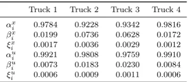
N = 25. Before applying Algorithm 1 to the system we obtain the scaling constants (αx
i, βix, ξxi)and (αui, βiu, ξiu)
for each trucki∈ M—see Table 1 for the values obtained through the procedure detailed in Section 5.
In Figure 1, the different scalings of the state constraint sets are shown for truck 2, and also the corresponding RCI sets. Thus, for truck 2,92.28%of the state constraint set is allocated to the the main optimal control problem, which is concerned with regulating the nominal subsystem (i.e., neglecting interactions). On the other hand, the ancillary problem—which regulates the planned errors—has
7.36% of the original state constraint sets. The remaining
0.36%of the state constraint set is allocated to the RCI control law to handle unplanned disturbances.
7. CONCLUSIONS
A distributed MPC algorithm for dynamically coupled linear systems was proposed. Subsystem controllers solve (once, at each time step) local optimal control problems to determine control sequences and state trajectories, and exchange information about these. The main feature of the proposed algorithm is the use of a secondary MPC controller for each subsystem, which acts on the shared
Table 1. Designed values of scaling factors.
Truck 1 Truck 2 Truck 3 Truck 4
αx
i 0.9784 0.9228 0.9342 0.9816
βx
i 0.0199 0.0736 0.0628 0.0172
ξx
i 0.0017 0.0036 0.0029 0.0012
αu
i 0.9921 0.9808 0.9759 0.9910
βu
i 0.0073 0.0183 0.0230 0.0084
ξu
i 0.0006 0.0009 0.0011 0.0006
plans of other subsystems and aims to reject the uncertainty caused by neglecting interactions in the main problems. Recursive feasibility and stability are guaranteed under provided assumptions, and a design methodology was given for the off-line selection of controller parameters and illustrated with an example.
A key advantage of the proposed approach, in addition to the guaranteed feasibility and stability and despite this being a tube-based method, is the absence of invariant sets in the optimal control problems. This makes the approach potentially applicable to higher-dimensional subsystems.
REFERENCES
Christofides, P.D., Scattolini, R., Muñoz del la Peña, D., and Liu, J. (2013). Distributed model predictive control: A tutorial review and future research directions.
Computers & Chemical Engineering, 51, 21–41. doi: 10.1016/j.compchemeng.2012.05.011.
Farina, M. and Scattolini, R. (2012). Distributed predictive control: A non-cooperative algorithm with neighbor-to-neighbor communication for linear systems. Automatica, 48, 1088–1096. doi:10.1016/j.automatica.2012.03.020. Hernandez, B. and Trodden, P. (2016). Distributed model
predictive control using a chain of tubes. InProceedings of the 2016 UKACC International Conference on Control (CONTROL 2016). (To appear).
Maestre, J.M. and Negenborn, R.R. (eds.) (2014). Dis-tributed Model Predictive Control Made Easy. Springer. Mayne, D.Q., Kerrigan, E.C., van Wyk, E.J., and Falugi, P. (2011). Tube-based robust nonlinear model predictive control. International Journal of Robust and Nonlinear Control, 21, 1341–1353. doi:10.1002/rnc.1758.
Mayne, D.Q., Seron, M.M., and Raković, S.V. (2005). Robust model predictive control of constrained linear systems with bounded disturbances. Automatica, 41(2), 219–224. doi:10.1016/j.automatica.2004.08.019.
Mayne, D.Q. (2014). Model predictive control: Recent developments and future promise. Automatica, 50, 2967– 2986. doi:10.1016/j.automatica.2014.10.128.
Raković, S.V., Kerrigan, E.C., Mayne, D.Q., and Koura-mas, K.I. (2007). Optimized robust control in-variance for linear discrete-time systems: Theoreti-cal foundations. Automatica, 43(5), 831–841. doi: 10.1016/j.automatica.2006.11.006.
Rawlings, J.B. and Mayne, D.Q. (2009). Model Predictive Control: Theory and Design. Nob Hill Publishing. Riverso, S. and Ferrari-Trecate, G. (2012).
Tube-based distributed control of linear constrained systems. Automatica, 48, 2860–2865. doi: 10.1016/j.automatica.2012.08.024.
Scattolini, R. (2009). Architectures for distributed and hierarchical Model Predictive Control – A re-view. Journal of Process Control, 19, 723–731. doi: 10.1016/j.jprocont.2009.02.003.
[image:8.595.73.258.685.766.2]