This is a repository copy of
Predictive control of intersegmental tarsal movements in an
insect.
.
White Rose Research Online URL for this paper:
http://eprints.whiterose.ac.uk/117229/
Version: Accepted Version
Article:
Costalago-Meruelo, A., Simpson, D.M., Veres, S.M. et al. (1 more author) (2017)
Predictive control of intersegmental tarsal movements in an insect. Journal of
Computational Neuroscience. ISSN 0929-5313
https://doi.org/10.1007/s10827-017-0644-x
[email protected] https://eprints.whiterose.ac.uk/ Reuse
Items deposited in White Rose Research Online are protected by copyright, with all rights reserved unless indicated otherwise. They may be downloaded and/or printed for private study, or other acts as permitted by national copyright laws. The publisher or other rights holders may allow further reproduction and re-use of the full text version. This is indicated by the licence information on the White Rose Research Online record for the item.
Takedown
If you consider content in White Rose Research Online to be in breach of UK law, please notify us by
PREDICTIVE CONTROL OF INTERSEGMENTAL TARSAL
MOVEMENTS IN AN INSECT
Alicia Costalago Meruelo
1, David M. Simpson
1, S. Veres
2and Philip L. Newland
31
Faculty of Engineering and the Environment, University of Southampton, Southampton, UK
2
Department of Automatic Control and Systems Engineering, University of Sheffield, Sheffield, UK
3
Biological Sciences, University of Southampton, Southampton, UK [email protected]
Keywords: Reflex, Artificial Neural Network, Time Delay Neural Network, Metaheuristic Algorithm, Evolutionary Programming, Particle Swarm Optimisation, Locust.
Abstract: In many animals intersegmental reflexes are important for postural control and movement making them ideal candidates for the bio-inspired design in developing treatment for neurological injuries such as drop foot and in robot design. Here we analyse an intersegmental reflex of the foot (tarsus) of the locust hind leg, which raises the tarsus when the tibia is flexed and depresses it when the tibia is extended. A novel method is described to measure and quantify the intersegmental responses of the tarsus to a stimulus to the femoro-tibial chordotonal organ. An Artificial Neural Network, the Time Delay Neural Network, was applied to understand the properties and dynamics of the reflex responses. The aim of the study was twofold: first to develop an accurate method to record and analyse the movement of an appendage and second, to apply methods to model the responses using Artificial Neural Networks. The results show that Artificial Neural Networks provide accurate predictions of tarsal movement when trained with an average reflex response to Gaussian White Noise stimulation compared to autoregressive models. Furthermore, the Artificial Neural Network model can predict the individual responses from each of the animals and responses to another input such as a sinusoid. A detailed understanding of such a reflex response could be included in the design of orthoses or functional electrical stimulation treatments to improve walking in patients with neuromuscular disorders.
1
INTRODUCTION
The impairment of motor function in disease and ageing is an issue that costs health services enormous sums each year (Hanson et al., 2006). Individuals with neuromuscular disorders, such as proprioceptive deficits, show degradation in movement (Goble et al., 2009) where they are unable to sense the static or dynamic position of a joint, or limb segment (Gandevia et al., 2002). Individuals who survive a stroke may be left with foot drop making it difficult for them to raise the front of the foot (Stewart, 2008), while patients who have suffered an amputation, need an improved understanding of neuromuscular control in healthy individuals to design better and optimised treatment, such as rehabilitation, or the use of prostheses and orthoses (He et al., 2001).
Studies of neuromuscular control are therefore important to understand how the nervous system generates and controls movements in any situation (Webb et al., 2004). Furthermore, features of
neuromuscular control can be exploited to improve the design of engineering control systems. The implementation of bio-inspired designs based on
neuromuscular control has made important
contributions in robotic engineering and autonomous systems (Delcomyn, 2004), such as an improved gait and stability during walking in robotics (DŸrr et al., 2004; Ijspeert, 2008; Lewinger et al., 2011; Webb, 2002).
needed in the autonomous control of walking robots, where irregular terrains and obstacle negotiation are still limited (Chen et al., 2011).
Here we develop methods to analyse and model control of an intersegmental reflex that consists of a movement of the tarsus around the tibio-tarsal joint in response to changes in the femoro-tibial joint angle (Burrows and Horridge, 1974) that is thought to increase stability and affect postural control (Burrows, 1996; Clarac et al., 1978). The movement is neurally mediated (Burrows and Horridge, 1974) by the Femoral-Chordotonal Organ (FeCO) at the femoro-tbial joint of the hind leg (Field and Burrows, 1982). Similar reflexes have evolved in other insects, such as the New Zealand Weta (Field and Rind, 1981), in stick insects (BŸschges and Gruhn, 2007; Cruse et al., 1992) and in crustaceans (Clarac et al., 1978) suggesting an underlying control principle in arthropods related to stability and posture control that is also found in some mammals (Halbertsma, 1983; Pearson, 1993).
This paper describes novel methods to record and quantify reflex responses in the locust hind leg tarsus, the application of a previously validated mathematical approach to model and predict
biologically source responses using ANNs
(Costalago Meruelo et al., 2016) and analyses variability between individuals and ask whether individual responses or an average response should be used to model and study the system.
2
METHODS
2.1
Experimental Methods
2.1.1 Video recordings
Adult male and female locusts (Schistocerca gregaria ForskŒl) were mounted in modelling clay ventral side up, with the left hind leg femur fixed at an angle of 30° to the abdomen and with the tibia free to move. All other legs, thorax, abdomen and head were fixed with modelling clay to prevent movement. The tibia was moved passively from 0° (fully flexed) to 180° (fully extended) and back to a fully flexed position. The movement was a passive step movement performed using a micromanipulator, stopping every 10° for 5 s. The tibio-tarsal angle was recorded every 10° of femoro-tibial joint angle. This procedure was repeated five times for each individual, and the individual responses averaged to reduce the intra-subject variability. To determine whether the tarsal intersegmental reflex contained a mechanical component or if it was purely neurally mediated, the same experiment was performed in each animal after nerve N5, containing the axons of motor neurons innervating leg muscles and sensory neurons (Burrows, 1996) was cut.
2.1.1 Shaker and laser recordings
Adult locusts were fixed in modelling clay ventral side up, with the femur fixed at 60¡ to the abdomen and with the tibia fixed at an angle of 60¡ to the femur, an angle which represents the middle of the linear range movement of the FeCO apodeme (Dewhirst et al., 2013)).
The FeCO was exposed by removing a small piece of cuticle at the distal end of the femur, and the cavity perfused with locust saline. The FeCO apodeme (Kondoh et al., 1995) was grasped with a pair of fine forceps attached to a shaker (permanent magnet shaker LDS V101). The shaker was driven by a signal generated in Matlab¨, which was amplified and converted to analogue via a digital-to-analogue converter (DAC) (USB 2527 data acquisition card (Measure Computing Norton, MA, USA). The movement of the tarsus was recorded with a Keyence laser displacement sensor (LK G3001V controller, LK G32 Head, Keyence) aimed at the last segment of the tarsus, the unguis.
The stimulus signals were designed and applied through Matlab¨. Locusts walk at a step frequency of approximately 3 Hz (Burrows and Horridge, 1974) and for this reason, Gaussian White Noise (GWN) was produced in the band-limited range between 0 - 5 Hz, and a sinusoidal input simulating walking was applied at 1 Hz. The maximum peak-to-peak amplitude of the input signals was approximately 1 mm, which represents a femoro-tibial displacement of 90¡ (Dewhirst et al., 2013; Field and Burrows, 1982). The signals were scaled so that approximately 99.7 % of their values fell within the femoro-tibial joint angle between 20¡ and 100¡ (0.9 mm of displacement of the FeCO apodeme). The frequency and phase response of the equiment was linear between 0 and 200 Hz.
Three versions of each 5 Hz band-limited GWN were created in MATLAB¨ using its pseudo random number generator, randn. This generated an array
of random numbers drawn from a Gaussian distribution with a standard deviation (σ) of one. Since a single GWN input would not cover all frequencies and amplitudes within the specified range, due to the relatively long time needed to cover the lowest frequencies (i.e. 0.1 Hz requires 10s for just one amplitude), three different band-limited GWN signals were created that covered the band of interest. This was created by low pass filtering using a 5th order Butterworth low pass filter with a cut-off frequency of 5 Hz, applied in the forward and reverse directions for zero phase shift.
2.1
Mathematical Methods
2.2.1 Data Post-Processing
500 Hz after applying an anti-alias filter, a third order Butterworth with a cut-off frequency of 200 Hz, thereby reducing file size and processing time. Both Butterworth filters were applied in the forward and reverse directions to avoid introducing any phase delay. An average reflex response was calculated using the responses from the eight individuals to test whether the average was representative of the system or if individual responses provided better models.
2.2.2 Artificial Neural Networks
To model the intersegmental reflex responses of the tarsus a dynamical artificial neural network, a Time Delay Neural Network (TDNN) (Waibel et al., 1989), was used. This network uses delayed versions of the input to estimate the output, turning the static Feed-Forward Network into a dynamic network (Haykin, 2004). Using this, we assumed the reflex responses to be a combination of current and past input samples. The network was formed by an input node, an output node, and a number of hidden layers and with hidden nodes and the activation function for each hidden node was the sigmoid. The output node had a linear function, so all the non-linear calculations were performed inside the network. The training algorithm for the network was the Levenberg-Marquadt back-propagation algorithm, which had higher accuracy and faster convergence time than classical back-propagation algorithms (Bishop et al., 1995). The number of delayed samples used in the input was set to 100 samples, which was based on preliminary work (optimisation of decrease in NMSE as the delay increases for a set architecture). The architecture of the network was optimised using a metaheuristic algorithm presented in the next section. The full description of the methodology for the network design and training is shown in previous work (Costalago Meruelo et al., 2016).
2.2.4 Autoregressive Model
To compare the results of the TDNN, an autoregressive (AR) model of the tarsal movements was developed. As with the TDNN, the model assumed that the tarsal response was a combination of current and past input samples. Considering the discrete form, the response of the system can be characterised as:
! ! ! ! ! ! ! ! ! ! ! !!!! !!!
!!!
(6)
Where ! ! is the response, ! ! is the transfer
function of the system, ! !! ! is the stimulus and !!!! is the noise. To calculate the parameters of !! ! the least square method was used. The equation of the Minimum Mean Square Error cost function (Haykin, 2004) is rearranged and it is assumed that the prediction is a linear function of the impulse response function. Combining the cost function with
the system response, the least square estimate of the AR parameters is:
! ! !!!!!!!!!! (7)
Where ! is the output, ! is the pre-windowed
matrix (Ljung, 1998) and ! the estimated model
parameters. For a full derivation see Dewhirst (2012). To compare the results from both mathematical models, the NMSE (Equation 2) was used, when the model was tested with the same data not used in training.
3
RESULTS
3.1
Intersegmental Reflex Responses
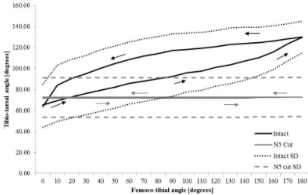
3.1.1 Static Intersegmental Reflex Responses Movement of the tibia to different fixed femoro-tibial angles led to tarsal positions dependent on femoro-tibial angle (Fig. 1). The average response of eight animals showed that the tibio-tarsal angle strongly depended on the femoro-tibial joint angle. As the tibia was extended, the tarsus was depressed and as the tibia was flexed the tarsus was levated, thereby maintaining a constant position relative to the abdomen, as shown by Burrows and Horridge (1974). A Spearman's rank correlation coefficient of the average response between the tibio-tarsal angle and the femoro-tibial angle was calculated and the results (r = 1.00, p < 0:001) for both extension and flexion of the tibia, confirmed that changes in the femoro-tibial joint angle and changes in the tibio-tarsal joint angle were correlated. The high significant correlation coefficients were constant for each individual tested (Table 1).
Figure 1. The average tarsal response to movement of the tibia about the femoro-tibial joint. Responses are shown for the intact leg and when nerve N5 was cut. There was a significant difference between the two responses (N5 intact and cut).
tibia, both could be represented, in part, through nonlinear regression. During extension of the tibia, the tarsus was depressed following a linear regression with a slope of β = 0.32 (R2 = 0.98, p < 0.001), suggesting an almost linear response below femoro-tibial angles of 150¡. During flexion of the tibia, the tarsus was elevated following a linear regression with slope of β = 0.29 (R2 = 0.85, p < 0.001). In this case, the tarsal response did not follow a straight line as in tibial flexion, indicating higher levels of non-linearity during flexion than during extension of the tibia.
The movements of the tarsus were not simply dependent on femoro-tibial joint angle, but also the direction from which an angle was approached. During extension, the tibio-tarsal angle increased gradually until the leg was fully extended, increasing faster near the fully extended tibial positions (above 150¡). During flexion the tibio-tarsal angle initially decreased slowly (small changes in tibio-tarsal angle to changes in femoro-tibial angle), but then faster after the tibia reached 60¡, and even faster for angles lower than 30¡.
Table 1. Spearman's rank correlation coefficients between femoro-tibial angles and tibio-tarsal angles for each of the individual animals and for the average response of all individuals (Avg resp). The probabilities for all correlation coefficients calculated were p< 0:001.
Animal 1 2 3 4 5 6 7 8 Avg resp Extensi
on
1.00 1.00 1.00 1.00 0.99 1.00 1.00 1.00 1.00
Flexion 0.92 1.00 0.99 1.00 0.99 1.00 0.98 0.99 1.00
To establish whether the reflex was purely neuronal or whether it contained a mechanical component, the experiment was repeated in each animal with nerve N5 severed. The results show that when nerve N5 was cut little movement of the tarsus was evident, however a Pearson's correlation test showed that there was a significant small movement of the tarsus to changes in femoro-tibial angle (r = 0.37, p = 0. 02). These changes, however, were significantly different from the large changes observed when nerve N5 was intact (p = 0.001). These results indicate that the tarsal intersegmental reflex control system was mainly neuronally mediated, with possibly a little mechanical coupling.
3.1.2 Laser Recordings of the Intersegmental Reflex Responses
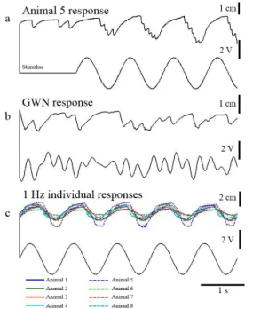
In response to a 1Hz sinusoidal stimulus applied to the FeCO the movements of the tarsus followed approximately the input (Fig. 2A), such that stretches of the FeCO apodeme, equivalent to a flexion of the tibia, evoked a levation of the tarsus, whereas relaxation of the apodeme, equivalent to tibial extension, evoked tarsal depression. These responses showed that tarsal depression (upward deflection of the trace) was smoother than tarsal levation (downward deflection of the trace), reflecting the activity of the underlying motor neuron activity,
which also resulted in spontaneous movements before the stimulus to the FeCO was applied.
In response to a 5 Hz band-limited GWN (Fig. 2B), tarsal movement did not follow the higher
frequency inputs, smoothing the response.
Movements of the tarsi from 8 different individuals to a 1 Hz stimulus applied to the FeCO showed that they have similar responses but with varying amplitudes. There was also an observable delay between the input to the FeCO and the movement of the tarsus of 0.1s, resulting from known neural conduction times and synaptic delays (Burrows, 1996, Endo et al., 2015).
3.2
Autoregressive
Model
of
the
Intersegmental Responses
The linear model of the average tarsal intersegmental response was calculated using the Autoregressive (AR) model described in Section 2.2.4. The parameters of the model were calculated using the first of the three 5 Hz band-limited GWN responses, averaged across the eight individuals (which in turn are the average of three recordings). One model for each individual response was calculated, as well as a model for the average response.
Figure 2. Intersegmental tarsal movements evoked by displacement of the FeCO. a) Movements of the tarsus of animal 5 to a 1 Hz sinusoidal stimulus. b) Movements of the tarsus of Animal 5 to a 5 Hz band-limited GWN stimulus. c) Movements of the tarsi of all eight individuals to a 1 Hz sinusoidal stimulus. An upward deflection of the tarsal movement traces represents tarsal depression.
The best performing model was the LSM model calculated for Animal 8, with a NMSE of 29.3 % for the GWN input. When the models were tested with 1 Hz inputs, the best performing model, however, was the one designed for Animal 1, which was the second worst at predicting GWN inputs (Table 3).
The LSM model calculated with the average response across all individuals was able to predict the average response better than any other individual model, with a NMSE = 27.2%, when tested with unseen data. The performance of this model with the average tarsal response to 1 Hz sinusoid was also better than with any of the individual responses, with a NMSE = 4.6%.
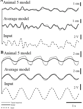
Figure 3. Least Square Model predictions of unseen 5 Hz band-limited GWN and 1 Hz sinusoidal inputs (dotted lines show the response while the black line the model). a) Prediction of the model for Animal 5 to 5 Hz GWN. b) Prediction of the model for the average tarsal response with 5 Hz band-limited GWN. c) 5 Hz band-limited GWN input. d) Prediction of the LSM for Animal 5 to a 1 Hz input. e) Prediction of the LSM for the average response to a 1 Hz input. f) 1 Hz sinusoidal input to the FeCO. The parameters of the model were calculated using a 5 Hz band-limited GWN tarsal response and tested with unseen data.
3.3 Artificial Neural Networks
3.3.1 Metaheuristic Algorithm TDNN
Architecture
Using the responses from the eight animals and the average response across all individuals to band-limited GWN, a metaheuristic algorithm (Costalago Meruelo et al., 2016) was run until the optimal architectures for each response were obtained (Table 2), with a total of 9 models. While the algorithm was set to a maximum of five layers and 32 nodes per layer, the optimal architectures were limited to two layers and a maximum of five nodes per layer. The
algorithm was set to run over 50 iterations or generations, however, the ANN architectures converged and the best or optimal network obtained after the 35th generation for all the individual responses, including the average response. We therefore assumed it had reached the maximum fitness within 35 generations.
Table 2. Number of nodes per layer for the TDNN designed using the metaheuristic algorithm.
Layer 1 Layer 2 Average response 4 -
Animal 1 3 -
Animal 2 5 -
Animal 3 5 1
Animal 4 2 1
Animal 5 3 1
Animal 6 3 -
Animal 7 4 -
Animal 8 3 -
3.3.2 TDNN models of the Intersegmental Responses
The TDNN models optimised for the individual and the average responses were tested using unseen GWN data and a sinusoidal input, none of which were used in the training or the algorithm. The models were able to approximate the response of the 5 Hz GWN and follow its trajectory, both in the case of the TDNN trained with recordings from Animal 5 and with the average response calculated across all animals (Fig. 4).
band-limited GWN. c) 5 Hz band-band-limited GWN input. d) Prediction of the TDNN for Animal 5 to a 1 Hz input. e) Prediction of the TDNN for the average response to a 1 Hz input. f) 1Hz sinusoidal input. The parameters of the model were calculated using a 5 Hz band-limited GWN tarsal response and tested with unseen data.
For a 1 Hz stimulus applied to the FeCO, it was clear that the model trained with Animal 5 was not able to predict the high amplitude movements of the tarsal responses in Animal 5, although the model trained with the average response could predict the average response to 1 Hz.
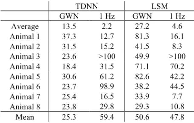
The TDNN models had lower NMSE than the LSM models for every individual, including the average response (Table 3). These NMSE values were calculated for TDNN models trained with a specific individual (or the average response across all individuals) and tested with unseen data from the same individual (or the average response). With a mean value of 25.3 %, the TDNN produced a better model than the LSM, with 50.6 %.
To corroborate whether the TDNN were better at predicting the tarsal responses, a paired samples t-test was applied, chosen for the normality of the data (Shapiro-Wilk Test, p = 0.881 for the TDNN models and p = 0.098 for the LSM models), despite the small sample size (9 samples in total, considering models for the 8 individuals and the average response across them). The results showed that the TDNN had a statistically significantly lower NMSE (25.3 ± 7.1 %, mean ± standard deviation) than the LSM models (50.6 ± 22.1 %), with t(16) = -3.924 and p < 0.01. This indicated that the TDNN were statistically significantly better at predicting the tarsal intersegmental responses. Since the sample size was small, and to compare with following statistical analysis, a Mann-Whitney U-test was applied. The results also confirmed that the performances of both models were statistically significantly different (U = 74.0, p < 0.01).
Table 3. NMSE of the individual models when tested with unseen GWN and 1 Hz sinusoidal inputs from the same individual as training, but not the same response as used in the training.
TDNN LSM
GWN 1 Hz GWN 1 Hz Average 13.5 2.2 27.2 4.6 Animal 1 37.3 12.7 81.3 16.1 Animal 2 31.5 15.2 41.5 8.3 Animal 3 23.6 >100 49.9 >100 Animal 4 18.4 31.5 71.1 70.2 Animal 5 30.6 61.2 82.6 42.2 Animal 6 23.7 98.9 38.2 44.5 Animal 7 25.4 16.5 33.9 7.7 Animal 8 23.8 29.8 29.3 10.8
Mean 25.3 59.4 50.6 47.8
To show the generalisation of such models when another input was applied, Figure 5 also shows the prediction of these networks when a sinusoidal
stimulus was applied. Table shows that the performance of the TDNN models was worse than the performance of the LSM (59.4 ± 74.4 % for the TDNN and 47.8 ± 62.9 % for the LSM). To determine whether this difference was statistically significant, a Mann-Whitney U test was applied to the data, since both models produce non-normal data (Shapiro-Wilk Test has a p = 0.00 < 0.05 for both the TDNN models and the LSM models, indicating that the data from both models was non-normal). The results from the test indicated that the performances of both models were not significantly different (U = 34.0, p = 0.61).
Therefore, the TDNN models are statistically better at predicting the responses to 5 Hz band-limited GWN than the LSM models, however they were not statistically different to them when predicting responses to a 1 Hz sinusoid.
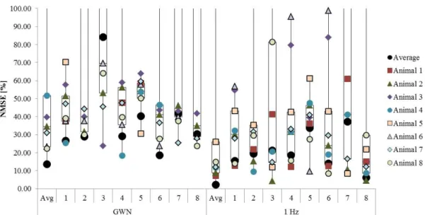
3.3.3 Generalisation of TDNNs to different individual responses
To analyse generalisation in more detail, the models trained with 5 Hz band-limited GWN were then tested with the responses from all individuals and the average of these (Fig. 5). Here, the term generalisation refers to the ability of the model to predict the tarsal reflex responses in different individuals that were not used in the training process. In Figure 5, each box-plot represents the NMSE of a specific model, trained with either the average response or the responses from individual animals (1-8). The NMSE was calculated when these models were applied to all the responses, represented by the different markers.
Results show that the models could predict well the responses from some individuals. The model from the average response was the best performing model while that of Animal 3 was the worst performing model. However, there were some responses that were poorly predicted by the models, such as the model of the average response that could not predict the GWN responses of Animal 5. The average response across all animals, however, was predicted by all the individual models (see black dots in Figure 5).
All individual models had a prediction error higher than 100 % when tested with Animal 5, with the exception of the model trained with Animal 5, and the model trained with Animal 1. The model trained with Animal 1 was able to predict all the responses from any individual, better than the model trained with the average response calculated across individuals, with the exception of the tests on recordings from Animal 3 and 8.
in the distribution (NMSE values higher than 100%), which bias estimates of mean and standard deviation.
Table 4: Mean and standard deviation of the NMSE values for each of the nine TDNN models. The NMSE value presented for each model was the mean of the NMSE values calculated with that model and averaged across all the individuals, including the average response.
GWN 1 Hz
Mean sd Mean sd
Average 55.9 52.7 47.7 64.4
Animal 1 43.6 14.6 31.9 16.7
Animal 2 82.2 77.8 69.8 97.2
Animal 3 219.6 271.5 109.4 175.3
Animal 4 48.6 24.5 40.0 28.9
Animal 5 52.1 10.5 38.0 14.4
Animal 6 57.5 49.7 37.0 32.7
Animal 7 119.8 141.8 146.3 226.6
Animal 8 102.2 124.0 62.1 101.2
Table 4 shows that the model trained with the responses from Animal 1 had lower performance error than any other model, while the model trained with the responses from Animal 3 has the highest errors, although this may only be true due to the NMSE values of the TDNN tested with Animal 5, which caused outliers. Surprisingly, the model trained with recordings from Animal 5 could predict all the individual responses with a low performance not much higher than the best performing model, considering that its responses could not be predicted by any other model.
To estimate whether the performances of the models were significantly different (i.e. the animal used for training data, or average response, had a
significant impact on the performance of the model), a Friedman test was chosen. This test was chosen because it analysed the differences in three or more groups of dependant variables (i.e. repeated tests from different animals within the same network) providing the results were continuous and the data non-parametric. The test was applied to the NMSE values obtained with GWN and 1 Hz separately. The test also gives some insight into the importance of the animal chosen to design the model, or whether the average across individuals could be used as a representation of the system.
The Friedman test was also chosen because of the non-normality of most of the data (the Shaphiro-Wilk tests have p < 0.05 for Animal 2, 3, 6, 7 and 8, and p < 0.001 for the overall data). Results indicated that the NMSE values were significantly different (2(8) = 21.9, p = 0.01) when the networks were tested with a 5 Hz band-limited GWN and when they were tested with 1 Hz sinusoid (2(8) = 15.3, p = 0.05). These statistical tests indicate that the training data used to design the networks affects significantly the performance of the model when predicting data from different individuals.
4
DISCUSSION
4.1
Tarsal intersegmental responsesUsing new approaches we have developed an extensive and quantitative analysis of an intersegmental reflex in which movement of the tarsus about the tibio-tarsal joint was mediated by changes in the position of the tibia about the femoro-tibial joint. As the leg was flexed, the apodeme of the FeCO was stretched and the tarsus levated, and when
the leg was extended, the apodeme was relaxed and the tarsus depressed. We then modelled the reflex movements of the tarsus using both Autoregressive and Artificial Neural Networks and showed that the models produced by the ANNs provided better predictions of the intersegmental responses. Finally, we then analysed the variability in responses of reflex movements between animals and asked how good the models from individual animals were in predicting the tarsal reflex movements in different animals.
Intersegmental tarsal reflexes are relatively common in the limbs of arthropods. Similar intersegmental reflexes have also been described in the New Zealand Weta, rock lobsters and crayfish (Bush et al., 1978; Clarac et al., 1978; El Manira et al., 1991; Field and Rind, 1981), where a response in one segment of the leg is initiated by a chordotonal organ in another leg segment. Surprisingly a similar reflex is not present in the limbs of stick insects
(Radnikow and BŠssler, 1991) despite the
innumerable similarities in their nervous systems (Bassler, 1977), where reflex responses can be elicited by a chordotonal organ in the same way as in locusts (Bucher et al., 2003; Hess and BŸschges, 1999, 1997). The function of such reflexes is still not fully understood, although it is believed to be a locomotory reflex rather than a stance reflex, aimed to facilitate centrally driven movements. Its function seems to be related to avoid catching the claws on the substrate while walking and pressing the tarsus onto the ground during the power phase of locomotion (Field and Rind, 1981). Similarly, the rock lobster also produces a reflex response that originates from the joint that produces the main power during the propulsive phase of a step (Clarac et al., 1978).
4.2 Artificial Neural Networks for system
identification in biological systems
Costalago Meruelo et al. (2016) described a novel method to model and predict neural responses using ANNs and to explore and understand such responses with a high degree of accuracy. The method used to design the ANN architecture, a combination of Evolutionary Algorithms and Particle Swarm Optimization (Eiben and Smith, 2003; John, 1992; Kennedy and Eberhart, 1995), optimised the architecture of the network to individual and averaged responses. The design of the optimal architecture was necessary to reduce computational time, improve prediction accuracy, reduce over-fitting and improve generalization capabilities (Angeline et al., 1994; Suraweera and Ranasinghe, 2008; Yao, 1999). A similar method used here, produced small networks with up to two hidden layers and a small number of nodes in each layer to model tarsal movements, although the networks were smaller for tarsal responses than for neural responses (Costalago Meruelo et al., 2016). The small size is thought to be better at generalising and in reducing over-fitting (Sietsma and Dow, 1991; Suraweera and Ranasinghe, 2008). Larger networks may produce a lower error in the training data, but are less able to
predict the responses to a novel stimulus. We showed here that the ANNs were able to outperform significantly previously used mathematical methods. For example, using ANNs the prediction error was reduced by approximately 10 % compared to the LNL methods (Dewhirst et al., 2013) and by 25 % compared to Wiener methods (Newland and Kondoh, 1997a,b). It should be pointed out. However, that such comparisons must be considered with caution, since it is not just the model structure or its type that affects the results, but also the size or number of model parameters that can impact the fit and ability to generalise. For tarsal intersegmental responses ANNs had approximately half the mean square error of the linear models suggesting than ANNs were better than linear models commonly used in biological systems (Marmarelis, 2004).
4.3 Individual variability in the tarsal
intersegmental reflex responses
Angarita-Jaimes et al. (2012) showed that the NMSE errors of models of motor neurons could not be ascribed only to modelling errors or background noise, but may also be due to individual differences of the same neuron between animals. Similarly, Schneidman and Brenner (2000), showed that in information rates in the visual system of flies that the common underlying response across individuals contributes about 70 % of the information recorded in the response, whereas the remaining 30 % comes from individual differences in the insect such as initial state, or inadvertent excitation of sensory neurons. Our results, similarly, show that there is a common response across all individuals, since all models were able to predict some (but not all) of the responses from other animals, independently of the animal used for training. Even so, the ability of each model to predict the responses from each of the animals was significantly different. These differences in the prediction errors can partly be explained by differences across animal responses, as a result of spontaneous activity found in central interneurons and motor neurons (Buschges et al., 1994; Field and Burrows, 1982), differences in parameters (Marder and Taylor, 2011) and electrical and cellular noise (Faisal et al., 2008).
4.4 Wider implications
current systems lack this adaptability due to being based on preprogrammed patterns (JimŽnez-Fabi‡n and Verlinden, 2012). Furthermore, robotics, autonomous systems and control already use direct applications of biological systems (Beer et al., 1997). In robotics, some of the most successful legged robots are based upon arthropods (Ritzmann et al., 2004), however, there design have raised issues related to the level of autonomy, stability and coordination (Bares, 1999). Local reflexes such as those seen in insects have, when implemented, been shown to successfully improve robot locomotion (Espenschied et al., 1996, 1993), since insects have the ability to deal with uneven terrain, a characteristic that robots aim to emulate (Chen et al., 2011; Cruse et al., 1998; Delcomyn and Nelson, 2000; Kovač et al., 2008; Lewinger et al., 2011).
ACKNOWLEDGEMENTS
Alicia Costalago Meruelo was supported by an EPRSC grant (EP/G03690X/1) from The Institute of Sound and Vibration Research and the Institute for Complex Systems Simulations at the University of Southampton.
REFERENCES
Angarita-Jaimes, N., Dewhirst, O.P., Simpson, D.M., Kondoh, Y., Allen, R., Newland, P.L., 2012. The dynamics of analogue signalling in local networks controlling limb movement. Eur. J. Neurosci. 36, 3269Ð3282.
Angeline, P.J., Saunders, G.M., Pollack, J.B., 1994. An evolutionary algorithm that constructs recurrent neural networks. IEEE Trans. Neural Networks. 5, 54Ð65. Au, S.K., Herr, H.M., 2008. Powered ankle-foot prosthesis.
IEEE Robot. Autom. Mag. 15, 52Ð59.
Bares, J. E. (1999). Dante II: Technical Description, Results, and Lessons Learned. Int. J. Robot. Res., 18(7), 621Ð649.
Bassler, U., 1977. Sense organs in the femur of the stick insect and their relevance to the control of position of the femur-tibia joint. J. Comp. Physiol. 121, 99Ð113. Beer, R.D., Quinn, R.D., Chiel, H.J., Ritzmann, R.E., 1997.
Biologically inspired approaches to robotics: what can we learn from insects? Commun. ACM 40, 30Ð38. Bishop, C.M., Lange, N., Ripley, B.D., 1995. Neural
networks for pattern recognition., J. Am. Statistical Assocn. Oxford University Press.
Bucher, D., Akay, T., DiCaprio, R. a, Buschges, A., 2003. Interjoint coordination in the stick insect leg-control system: the role of positional signaling. J. Neurophysiol. 89, 1245Ð1255.
Burrows, M., 1996. The Neurobiology of an Insect Brain, Oxford University Press, Oxford.
Burrows, M., Horridge, G. a, 1974. The organization of inputs to motoneurons of the locust metathoracic leg. Philos. Trans. R. Soc. Lond. B. Biol. Sci. 269, 49Ð94. BŸschges, A., Gruhn, M., 2007. Mechanosensory Feedback
in Walking: From Joint Control to Locomotor Patterns. In Insect Mechanics and Control. Academic Press, pp. 193Ð230.
Buschges, A., Kittmann, R., Schmitz, J., 1994. Identified nonspiking interneurons in leg reflexes and during walking in the stick insect. J. Comp. Physiol. A 174, 685Ð700.
Bush, B.M., Vedel, J.P., Clarac, F., 1978. Intersegmental reflex actions from a joint sensory organ (CB) to a muscle receptor (MCO) in decapod crustacean limbs. J. Exp. Biol. 73, 47Ð63.
Chen, D., Yin, J., Zhao, K., Zheng, W., Wang, T., 2011. Bionic mechanism and kinematics analysis of hopping robot inspired by locust jumping. J. Bionic Eng. 8, 429Ð439.
Clarac, F., Vedel, J.P., Bush, B.M., 1978. Intersegmental reflex coordination by a single joint receptor organ (CB) in rock lobster walking legs. J. Exp. Biol. 73, 29Ð 46.
Costalago Meruelo, A., Simpson, D.M., Veres, S.M., Newland, P.L., 2016. Improved system identification using artificial neural networks and analysis of individual differences in responses of an identified neuron. Neural Networks 75, 56Ð65.
Cruse, H., Dautenhahn, K., Schreiner, H., 1992. Coactivation of leg reflexes in the stick insect. Biol. Cybern. 67, 369Ð375.
Cruse, H., Kindermann, T., Schumm, M., Dean, J. and Schmitz, J., 1998. WalknetÑa biologically inspired network to control six-legged walking. Neural networks, 11(7), pp.1435-1447.
Delcomyn, F., 2004. Insect walking and robotics. Ann. Rev. Entomol. 49, 51Ð70.
Delcomyn, F., Nelson, M.E., 2000. Architectures for a biomimetic hexapod robot. Rob. Auton. Syst. 30, 5Ð15. Dewhirst, O.P., 2012. Nonlinear System Analysis of Local
Reflex Control of Locust Hind Limbs by (DISS). University of Southampton.
Dewhirst, O.P., Angarita-Jaimes, N., Simpson, D.M., Allen, R., Newland, P.L., 2013. A system identification analysis of neural adaptation dynamics and nonlinear responses in the local reflex control of locust hind limbs. J. Comput. Neurosci. 34, 39Ð58.
DŸrr, V., Schmitz, J., Cruse, H., 2004. Behaviour-based modelling of hexapod locomotion: Linking biology and technical application. Arthropod Struct. Dev. 33(3), 237-250.
Eiben, a. E.A., Smith, J.J., 2003. Introduction to evolutionary computing. Springer Science & Business Media.
El Manira, A., DiCaprio, R.A., Cattaert, D., Clarac, F., 1991. Monosynaptic interjoint reflexes and their central modulation during fictive locomotion in crayfish. Eur. J. Neurosci. 3, 1219Ð1231.
Endo, W., Maciel, C, Simpson, D. and Newland, P.L., 2015. Delayed mutual information infers patterns of synaptic connectivity in a proprioceptive neural network. J. Computational Neurosci. 38, 427-438. Espenschied, K.S., Chiel, H.J., Quinn, R.D., Beer, R.D.,
1993. Leg coordination mechanisms in the stick insect applied to hexapod robot locomotion. Adapt. Behav. 1, 455Ð468.
Espenschied, K.S., Quinn, R.D., Beer, R.D., Chiel, H.J., 1996. Biologically based distributed control and local reflexes improve rough terrain locomotion in a hexapod robot. Rob. Auton. Syst. 18(1-2), 59-64.
Faisal, A., Selen, L.P.J., Wolpert, D.M., 2008. Noise in the nervous system. Nat. Rev. Neurosci. 9, 292Ð303. Field, L., Burrows, M., 1982. Reflex effects of the femoral
chordotonal organ upon leg motor neurones of the locust. J. Exp. Biol. 101, 265Ð285.
leg reflexes. Comparative Biochemistry and Physiology - Part A: Physiology, 68(1), 99Ð102. Gandevia, S.C., Refshauge, K.M., Collins, D.F., 2002.
Proprioception: Peripheral Inputs and Perceptual Interactions BT - Sensorimotor Control of Movement and Posture. In: Gandevia, S.C., Proske, U., Stuart, D.G. (Eds.) . Springer , Boston, MA, USA pp. 61Ð68. Goble, D.J., Coxon, J.P., Wenderoth, N., Van Impe, A.,
Swinnen, S.P., 2009. Proprioceptive sensibility in the elderly: Degeneration, functional consequences and plastic-adaptive processes. Neurosci. Biobehav. Rev. 33(3), 271Ð278.
Halbertsma, J.M., 1983. The stride cycle of the cat: the modelling of locomotion by computerized analysis of automatic recordings. Acta Physiol. Scand. Suppl. 521, 1Ð75.
Hanson, M.A., Burton, A.K., Kendall, N.A.S., Lancaster, R.J., Pilkington, A., 2006. The costs and benefits of active case management and rehabilitation for musculoskeletal disorders (RPRT). London, UK: Prepared by Hu-Tech Associates Ltd for the Health and Safety Executive.
Haykin, S., 2004. Neural Networks: A Comprehensive Foundation. Neural Networks 2nd Edition.
He, J., Maltenfort, M.G., Wang, Q.W.Q., Hamm, T.M., 2001. Learning from biological systems: modeling neural control. Control Syst. IEEE. 21(4), 55-69. Hess, D., BŸschges, a, 1997. Sensorimotor pathways
involved in interjoint reflex action of an insect leg. J. Neurobiol. 33, 891Ð913.
Hess, D., BŸschges, A, 1999. Role of proprioceptive signals from an insect femur-tibia joint in patterning motoneuronal activity of an adjacent leg joint. J. Neurophysiol. 81, 1856Ð1865.
Ijspeert, A.J., 2008. Central pattern generators for locomotion control in animals and robots: A review. Neural Networks 21, 642Ð653.
JimŽnez-Fabi‡n, R., Verlinden, O., 2012. Review of control algorithms for robotic ankle systems in lower-limb orthoses, prostheses, and exoskeletons. Med. Eng. Phys. 34, 397Ð408.
Holland, J. H. (1975). Adaptation in Natural and Artificial Systems. University of Michigan Press. GEN, MIT Press, Cambridge, MA.
Kennedy, J., Eberhart, R., 1995. Particle swarm optimization. In: Proceedings of ICNNÕ95 - International Conference on Neural Networks. IEEE, pp. 1942Ð1948.
Kondoh, Y., Okuma, J., Newland, P.L., 1995. Dynamics of neurons controlling movements of a locust hind leg: Wiener kernel analysis of the responses of proprioceptive afferents. J. Neurophysiol. 73, 1829Ð 1842.
Kovač, M., Fuchs, M., Guignard, A., Zufferey, J.C., Floreano, D., 2008. A miniature 7g jumping robot. In: Proceedings - IEEE International Conference on Robotics and Automation. pp. 373Ð378.
Lewinger, W. a, Reekie, H.M., Webb, B., 2011. A Hexapod Robot Modeled on the Stick Insect,. In: IEEE 15th International Conference on Advanced Robotics: New Boundaries for Robotics. pp. 541Ð548.
Ljung, L., 1998. System identification. In: Signal Analysis and Prediction. Springer, pp. 163Ð173.
Marder, E., Taylor, A.L., 2011. Multiple models to capture the variability in biological neurons and networks. Nat. Neurosci. 14, 133Ð138.
Marmarelis, V.Z., 2004. Nonlinear dynamic modeling of physiological systems. John Wiley & Sons.
Newland, P., Kondoh, Y., 1997a. Dynamics of neurons controlling movements of a locust hind leg II. Flexor tibiae motor neurons. J. Neurophysiol. 77(4), 1731-1746.
Newland, P.L., Kondoh, Y., 1997b. Dynamics of neurons controlling movements of a locust hind leg. III. Extensor tibiae motor neurons. J. Neurophysiol. 77(6), 3297Ð3310.
Pearson, K.G., 1993. Common principles of motor control in vertebrates and invertebrates. Annu. Rev. Neurosci. 16, 265Ð297.
Pearson, K.G., 1995. Proprioceptive regulation of locomotion. Curr. Opin. Neurobiol. 5(6), 786Ð791 Radnikow, G., BŠssler, U., 1991. Function of a muscle
whose apodeme travels through a joint moved by other muscles: why the retractor unguis muscle in stick insects is tripartite and has no antagonist. J. Exp. Biol. 99, 87Ð99.
Ritzmann, R.E., BŸschges, A., 2007. Adaptive motor behavior in insects. Curr. Opin. Neurobiol. 17(6), 629-636.
Ritzmann, R.E., Quinn, R.D., Fischer, M.S., 2004. Convergent evolution and locomotion through complex terrain by insects, vertebrates and robots. Arthropod Struct. Dev. 33(3), 361-379.
Rushton, D., 1997. Functional electrical stimulation. Physiol. Meas. 18(4), 241.
Schneidman, E., Brenner, N., 2000. Universality and individuality in a neural code. arXiv Prepr. Physics. Shultz, A., Lawson, B., Goldfarb, M., 2015. Variable
Cadence Walking and Ground Adaptive Standing with a Powered Ankle Prosthesis. IEEE Trans. Neural Syst. Rehabil. Eng. 1Ð1.
Sietsma, J., Dow, R.J.F., 1991. Creating artificial neural networks that generalize. Neural networks 4, 67Ð79. Stewart, J.D., 2008. Foot drop: where, why and what to do?
Pract. Neurol. 8, 158Ð169.
Suraweera, N.P., Ranasinghe, D.N., 2008. A natural algorithmic approach to the structural optimisation of neural networks. In: Proceedings of the 2008 4th International Conference on Information and Automation for Sustainability, ICIAFS 2008. pp. 150Ð 156.
Waibel, A., Hanazawa, T., Hinton, G., Shikano, K., Lang, K.J., 1989. Phoneme recognition using Time-Delay neural networks. IEEE Trans. Acoust. speech signal Process. 37, 328Ð339.
Webb, B., 2002. Robots in invertebrate neuroscience. Nature 417, 359Ð363.
Webb, B., Harrison, R. R., & Willis, M. A. (2004). Sensorimotor control of navigation in arthropod and artificial systems. Arthropod Structure and Development. 33(3), 301-329.