An efficient clustering algorithm for partitioning Y short tandem repeats data

R E S E A R C H A R T I C L E

Open Access

An efficient clustering algorithm for partitioning

Y-short tandem repeats data

Ali Seman

, Zainab Abu Bakar

and Mohamed Nizam Isa

Abstract

Background:Y-Short Tandem Repeats (Y-STR) data consist of many similar and almost similar objects. This characteristic of Y-STR data causes two problems with partitioning: non-unique centroids and local minima problems. As a result, the existing partitioning algorithms produce poor clustering results.

Results:Our new algorithm, calledk-Approximate Modal Haplotypes (k-AMH), obtains the highest clustering accuracy scores for five out of six datasets, and produces an equal performance for the remaining dataset.

Furthermore, clustering accuracy scores of 100% are achieved for two of the datasets. Thek-AMH algorithm records the highest mean accuracy score of 0.93 overall, compared to that of other algorithms:k-Population (0.91),

k-Modes-RVF (0.81), New Fuzzyk-Modes (0.80),k-Modes (0.76),k-Modes-Hybrid 1 (0.76),k-Modes-Hybrid 2 (0.75), Fuzzyk-Modes (0.74), andk-Modes-UAVM (0.70).

Conclusions:The partitioning performance of thek-AMH algorithm for Y-STR data is superior to that of other algorithms, owing to its ability to solve the non-unique centroids and local minima problems. Our algorithm is also efficient in terms of time complexity, which is recorded asO(km(n-k)) and considered to be linear.

Keywords:Algorithms, Bioinformatics, Clustering, Optimization, Data mining

Background

Y-Short Tandem Repeats (Y-STR) data represent the num-ber of times an STR motif repeats on the Y-chromosome. It is often called the allele value of a marker. For ex-ample, if there are eight allele values for the DYS391 marker, the STR would look like the following frag-ments: [TCTA] [TCTA] [TCTA] [TCTA] [TCTA] [TCTA] [TCTA] [TCTA]. The number of tandem repeats has effectively been used to characterize and differentiate between two people.

In modern kinship analyses, the Y-STR is very useful for distinguishing lineages and providing information about lineage relationships [1]. Many areas of study, in-cluding genetic genealogy, forensic genetics, anthropo-logical genetics, and medical genetics, have taken advantage of the Y-STR method. For example, it has been used to trace a similar group of Y-surname projects to support traditional genealogical studies, e.g., [2-4].

Further, in forensic genetics, the Y-STR is one of the pri-mary concerns in human identification for sexual assault cases [5], paternity testing [6], missing persons [7], human migration patterns [8], and the reexamination of ancient cases [9].

From a clustering perspective, the goal of partitioning Y-STR data is to group a set of Y-Y-STR objects into clusters that represent similar genetic distances. The genetic dis-tance of two Y-STR objects is based on the mismatch results from comparing the Y-STR objects and their modal haplotypes. For Y-surname applications, if two people share 0, 1, 2, and 3 allele value mismatches for each mar-ker, they are considered to be the most familially related. Furthermore, for Y-haplogroup applications, the number of mismatches is variant and greater than that typically found in Y-surname applications. This is because the hap-logroup application is based on larger family groups branched out from the same ancestor, covering certain geographical areas and ethnicities throughout the world. The established Y-DNA haplogroups named by the letters A to T, with further subdivisions using numbers and lower case letters, are now available for reference (see [10] and [11] for details).

* Correspondence:[email protected]

1_{Center for Computer Sciences, Faculty of Computer and Mathematical}

Sciences, Universiti Teknologi MARA (UiTM), 40450 Shah Alam, Selangor, Malaysia

Full list of author information is available at the end of the article

Efforts to group Y-STR data based on genetic distances have recently been reported. For example, Schlechtet al. [12] used machine learning techniques to classify Y-STR fragments into related groups. Furthermore, Semanet al. [13-19] used partitional clustering techniques to group Y-STR data by the number of repeats, a method used in genetic genealogy applications. In this study, we continue efforts to partition the Y-STR data based on the parti-tional clustering approaches carried out in [13-19]. Re-cently, we have also evaluated eight partitional clustering algorithms over six Y-STR datasets [19]. As a result, we found that there is scope to propose a new partitioning algorithm to improve the overall clustering results for the same datasets.

A new partitioning algorithm is required to handle the characteristics of Y-STR data, thus producing better clustering results. Y-STR data are slightly unique com-pared to the common categorical data used in [20-25]. The Y-STR data contain a higher degree of similarity of Y-STR objects in their intra-classes and inter-classes. (Note that the degree of similarity is based on the mis-match results when comparing the objects and their modal haplotypes.) For example, many Y-STR surname objects are found to be similar (zero mismatches) and almost similar (1, 2, and 3 mismatches) in their intra-classes. In some cases, the mismatch values of inter-class objects are not obviously far apart. Y-STR hap-logroup data contain similar, almost similar, and also quite distant objects. Occasionally, the Y-STR hap-logroup data may include sub-classes that are sparse in their intra-classes.

Partitional clustering algorithms

Classically, clustering has been divided into hierarchical and partitional methods. The main difference between the two is that the hierarchical method breaks the data up into hierarchical clusters, whereas the partitional method divides the data into mutually disjoint partitions. The pillar of the partitional algorithms is the k-Means algorithm [26], introduced almost four decades ago. As a consequence, the k-Means paradigm has been extended to various versions, including the k-Modes algorithm [25] for categorical data.

Thek-Modes algorithm owes its existence to the inef-fectiveness of the k-Means algorithm for handling cat-egorical data. Ralambondrainy [27] attempted to rectify this using a hybrid numeric–symbolic method based on the binary characters 0 and 1. However, this approach suffered from an unacceptable computational cost, par-ticularly when the categorical attributes had many cat-egories. Since then, a variety ofk-Modes-type algorithms have been introduced, such as k-Modes with new dis-similarity measures [21,22],k-Population [23], and a new Fuzzyk-Modes [20].

Partitional algorithms use an objective function in their optimization process, and the determination of this func-tion was described as the P problem by Bobrowski and Bezdek [28] and Salim and Ismail [29]. When he proposed thek-Modes clustering algorithm, Huang [25] splitPinto P1 and P2. P1 denotes the minimization problem of

obtaining values for the partition matrix wli of 0 or 1

(for the hard clustering approach) or 0 to 1 (for the fuzzy clustering approach); see Eq. (1b) as an example. Further-more,P2denotes the minimization problem of obtaining

the value that occurs most often (or the mode of a cat-egorical data set) to represent the center of a cluster (often called the centroid). The minimization ofP2by obtaining

the appropriate mode essentially causes the minimization of problem P2, and vice versa. As an example of the

optimization process for problemPin the Fuzzyk-Modes algorithm, we wish to solve Eq. (1) subject to Eqs. (1a), (1b), and (1c).

P Wð ;ZÞ ¼Xk_l¼1Xn_i¼1w∝lid Xð i;ZlÞ ð1Þ

subject to:

X_k

l¼1wli¼1;1≤i≤n; ð1aÞ

wli∈½0;1;1≤i≤n;1≤l≤k ð1bÞ

And

0<Xn

i¼1wli<n;1≤l≤k ð1cÞ

where:

wliis a (k×n) partition matrix that denotes the degree of membership of objectiin thelth cluster that contains a value of 0 to 1,

k (≤n)is a known number of clusters,

Zis the centroid such that[Z1, Z2,. . .,Zk]∊Rmk, α∊[1,∞) is a weighting exponent,

d(Xi,Zl) is the distance measure between the object

Xiand the centroidZl, as described in Eqs. (2) and (2a).

d xð ;zÞ ¼Xn_j¼1δ xj;zj

ð2Þ

where:

δ xj;zj

¼ 0;xj¼zj 1;xj≠zj

ð2aÞ

Huang and Ng [24] described the optimization process of_P1andP2as follows:

ProblemP1: FixZ=Z^ and solve the reduced problem

wli¼

1; If Xi¼Z^l 0; If Xi¼Z^h;h≠l

1 Xk

h¼1 d Xi;Z^l

d Xi;Z^h

" #1

α1

ð Þ

; If Xi≠Z^l;and Xi≠X^h;1≤h≤k ,

8 > > > > < > > > > :

ð3Þ

ProblemP2: FixW=Ŵand solve the reduced problemP(Ŵ, Z)as in Eq. (4) subject to Eq. (4a). This process obtains the most frequent attributes, or the modes, which give the centroids.

Zli¼að Þjp∈DOM Aj ð4Þ

where:

X

i;x

i;j¼að Þ_jp

w∝_li ≥ X_i;x i;j¼að Þ_jt

w∝_li ∀l;1 ≤ t ≤ nj; 1 ≤ ≤ m

ð4aÞ

andα∈[1,∞) is a weighting exponent.

Problem of partitioning Y-STR data

Due to the characteristics of Y-STR data, there are two optimization problems for existing partitional algo-rithms: non-unique centroids and local minima pro-blems. These two problems are caused by the drawback of the modes mechanism of determining the centroids. Non-unique centroids would result in empty clusters, whereas the local minima problem leads to poorer

clustering results. Both problems are a result of the obtained centroids, which are not sufficient to represent their classes.

Therefore, problems will occur for the following two cases:

i)The total number of objects in a dataset is small while the number of classes is large. To illustrate this case, consider the following example.

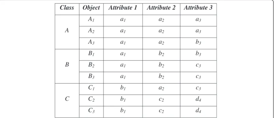
Example I: Figure 1 shows an artificial example of a dataset consisting of nine objects in three classes: Class A = {A1, A2, A3}, ClassB = {B1, B2, B3}, and Class C=

{C1, C2, C3}. Each object is composed of three attributes,

represented in lower case; e.g., for object A1, the

attri-butes are a1, a2, and a3. The dataset is considered to

have a higher degree of similarity between objects in intra-classes, while the number of objects is small and number of classes is large. Thus, the appropriate modes for representing the classes are: Class A – [a1, a2, a3],

lassB–[a1, b2, c3], and ClassC–[b1, c2, d4]. However,

attributea1in DOMAIN (A1),a2in DOMAIN (A2), and

c3in DOMAIN (A3) are too dominant, and would

there-fore dominate the process of updating P2. Figure 2

shows the possibility that each cluster is formed by the dominant attributes.

As a result, the mode that consists of [a1, a2, c3]

would be obtained twice. Thus, P2would not be

mini-mized due to this non-unique centroid. Another possi-bility is that the two modes are different, but are not distinctive enough to represent their clusters, such as modes [a1, a2, a3] or [a1, a2, b3] for Cluster 2. As a

consequence, this case would fall into a local minima problem.

Class

Object

Attribute 1

Attribute 2

Attribute 3

A

A

a

a

a

A

a

a

a

A

a

a

b

B

B

a

b

b

B

a

b

c

B

a

b

c

C

C

b

a

c

C

b

c

d

C

b

c

d

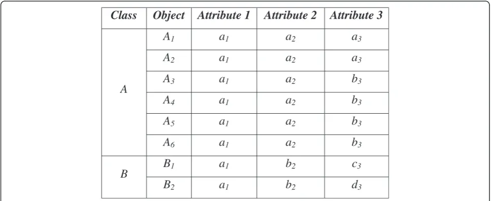
ii)An extreme distribution of objects in a class. To illustrate this case, consider the following example.

Example II:Figure 3 shows a dataset consisting of eight objects in two classes: ClassA= {A1, A2, A3, A4, A5, A6}

and ClassB= {B1, B2}. Each object consists of three

attri-butes, again represented in lower case. The appropriate modes to represent the classes are: Class A–[a1, a2, b3]

and ClassB–[a1, b2, c3] or [a1, b2, d3]. The distribution of

objects in Class Ais considerably larger than in Class B,

covering approximately 75% of the total set of objects. This characteristic of the data is found to be problematic forP2, particularly for the fuzzy approach. The problem is

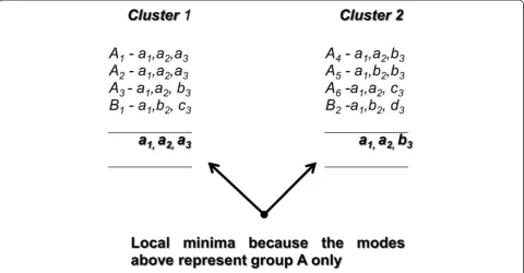
actually caused by the initial centroid selection. Figure 4 shows the objects in ClassAwould be equally distributed into clusters 1 and 2.

As a result, objectAbecomes dominant in both clusters, and so the obtained modes might be represented solely by objects in ClassA, e.g., [a1, a2, a3] and [a1, a2, b3].

Figure 2The dominant attributes form centroid 1 (a1, a2, c3),centroid 2 (a1, a2, c3) and centroid 3 (b1, c2, d3).In this case, there are

possibilities that each cluster is formed by the dominant attributes, e.g. attributea1,a2andc3.This scenario of non-unique centroids would result in empty clusters; otherwise the centroids would lead to local a minima problem and produce poorer clustering results.

Class

Object

Attribute 1

Attribute 2

Attribute 3

A

A

a

a

a

A

a

a

a

A

a

a

b

A

a

a

b

A

a

a

b

A

a

a

b

B

B

a

b

c

B

a

b

d

The above situations causePnot to be fully optimized, thus producing poor clustering results. Therefore, a new algorithm with a new concept ofP2is proposed in order

to overcome these problems and improve the clustering accuracy results of Y-STR data.

Methods

The center of a cluster

The mode mechanism for the center of a cluster (problem P2) is not appropriate for handling the characteristics of

Y-STR data, and therefore, it cannot be used as a mechan-ism to represent the center of a cluster (centroid). Instead, the center of Y-STR data should be the modal haplotypes, which are required to calculate the distance of Y-STR objects. The distance between a Y-STR object and its

modal haplotype can be formalized as in Eq. (5) subject to Eq. (5a).

dystrðX;HÞ ¼

X_m

j¼1 xj;hj

ð5Þ

subject to:

y xj;hj

¼ 0;xj¼ hj

1;xj≠ hj

ð5aÞ

wheremis the number of markers.

The modal haplotype is controlled by groups of objects that are similar or almost similar in Y-STR data. The similar and almost similar objects have a lower dis-tance, or a higher degree of membership values in a fuzzy sense. Thus, these two groups are considerably the Figure 4The extreme distribution of objectsAforms centroid 1 (a1,a2,a3) and centroid 2 (a1,a2,b3).In this case, the objects in Class A

are equally distributed into clusters 1 and 2. Therefore, the obtained centroids are not sufficient to represent their classes.

Table 1 Example of dominant objects

Objects Membership Values Probability of being the dominant object in the cluster

c1 c2 c1 c2

x1 0.7 0.3 100% (1.0) 50% (0.5)

x2 0.4 0.6 50% (0.5) 100% (1.0)

x3 0.6 0.4 100% (1.0) 50% (0.5)

most dominant objects required to find the Approximate Modal Haplotype. Consider four objects x1, x2, x3, and

x4and two clusters c1andc2. The membership value for

each object and its cluster are as shown in Table 1, whereby objectsx1and x3have a 100% chance of being

the most dominant object in cluster c1, but only a 50%

chance of being the dominant object in cluster c2, and

so on. A dominant weighting value of 1.0 is given to any dominant object and a weight of 0.5 is given to the remaining objects.

Thek-AMH algorithm

LetX ={X1, X2,. . ., Xn} be a set ofnY-STR objects and

A={A1,A2,. . ., Am} be a set of markers (attributes) of a

Y-STR object. Let H= {H1, H2,..,Hk} ∈ X be the set of

Approximate Modal Haplotypes for k clusters. Sup-pose k is known a priori. Let Hl be the Approximate

Modal Haplotype, represented as [hl,1, hl,2,. . .,hl,m],

and therefore, Hl,j = Xi,j for 1≤ j ≤ m and 1≤ i ≤ n.

The objective of the algorithm is to partition the cat-egorical objects X into kclusters. Thus, the Hl can be

replaced by Xiuntil nprovided they satisfy the

condi-tion described in Eq. (6).

P A s> P A t;s ≠ t; ∀t; 1 ≤ _t ≤ ð_nkÞ: ð6Þ

Here,P(Á)is the cost function described in Eq. (7), which is subject to Eqs. (7a), (8), (8a), (8b), (9), (9a), (9b), and (9c).

P A ¼ Xk_l¼1Xn_i¼1Ali ð7Þ

subject to:

Ali¼Wli∝Dli ð7aÞ

Wli∝is a (k×n) partition matrix that denotes the degree of membership of Y-STR objectiin thelth cluster that contains a value of 0 to 1 as described in Eq. (8), subject to Eqs. (8a) and (8b).

subject to:

w∝_li ∈ ½0;1; 1 ≤ i ≤ n; 1 ≤ l ≤ k; ð8aÞ

and

0 < Xn

i¼1w

∝

li < n; 1 ≤ l ≤ k ð8bÞ

where,

_{k (}≤n)is a known number of clusters.

_His the Approximate Modal Haplotype (centroid) such that[H1, H2,. . .,Hk]∈X.

α∈[1,∞) is a weighting exponent and used to increase the precision of the membership degrees. Note that this alpha is typical based on 1.1 until 2.0 as introduced by Huang and Ng [24].

_dystr(Xi,Hl) is the distance measure between the Y-STR objectXiand the Approximate Modal HaplotypeHl as described in Eq. (5) and subject to Eq.(5a). _Dliis another (k×n) partition matrix which

contains a dominant weighting value of 1.0 or 0.5, as explained above (See Table1). The dominant weighting values are based on the value ofWli∝ above.Dliis described in Eq. (9), subject to Eqs. (9a), (9b), and (9c).

dli ¼ 1:0; if w ∝

li ¼ maxw

∝

li;1 ≤ l ≤ k 0:5; otherwise

ð9Þ

subject to:

dli ∈ f1;0:5g; 1 ≤ i ≤ n; 1 ≤ l k ð9aÞ

1:5 ≤ Xk

l¼1dli ≤ k; 1 ≤ i ≤ n ð9bÞ

1:5 ≤ Xk

l¼1dli ≤ n; 1 ≤ i ≤ k ð9cÞ

Wli∝ ¼

1; If; Xi ¼ Hi

0; If; Xi ¼ Hz;z ≠ l

1 Xk

z¼1

dystr Xi;Hl

dystrðXi;HzÞ

1

∝1 ð Þ

; If Hi ≠ Xj and Xi ≠ Hz; 1 ≤ z ≤ k

, 0 B B B @

1 C C C A ∝ 8

> > > > < > > > > :

The basic idea of the k-AMH algorithm is to find k clusters in n objects by first randomly selecting an ob-ject to be the Approximate Modal Haplotype h for each cluster. The next step is to iteratively replace the objects x one-by-one towards the Approximate Modal Haplotype h. The replacement is based on Eq. (6) if the cost function as described in Eq. (7) and subject to (7a), (8), (8a), (8b), (9), (9a), (9b) and, (9c) is maxi-mized. Thus, the differences between the k-AMH algo-rithm and the other k-Mode-type algorithms are as follows.

i. The objects (the data themselves) are used as the centroids instead of modes. Since the distance of Y-STR objects is measured by comparing the objects and their modal haplotypes, we need to approximately find the objects that can represent the modal haplotypes. In finding the final Approximate Modal Haplotype for a particular group (cluster), each object needs to be tested one-by-one and replaced on a maximization of a cost function.

ii. A maximization process of the cost function is required instead of minimizing it as in thek -mode-type algorithms.

A detailed description of the k-AMH algorithm is given below.

Step 1–Select k initial objects randomly as Approximate Modal Haplotype (centroids).

E.g. if k= 4, then choose randomly 4 objects as the initial Approximate Modal Haplotype.

Step 2–Calculate distancedystr(Xi,Hl) according to Eq. (5) and subject to (5a).

Step 3–Calculate partition matrix wli∝ according to Eq. (8), subject to Eqs. (8a) and (8b). Note that the wli∝ is based on the distance calculated in Step 2.

Step 4–Assign a weighting dominant of 1.0 or 0.5 for partition matrixDliaccording to Eqs. (9), (9a), (9b) and (9c).

Step 5–Calculate cost functionP(Á) based onWli∝Dli according to Eqs (7) and (7a).

Step 6–Test for each initial modal haplotype by the other objects one-by-one. If current cost function is greater than previous cost function according to Eq. (6), then replace it.

Step 7–Repeat Step 2 until Step 6 for eachxandh

Step 8–Once the final Approximate Modal

Haplotypes are obtained for all clusters, assign the objects to their corresponding crisp clusters

Cliaccording to Eq. (10).

Cli ¼ 1; if l ¼ arg max w

∝

li ; 1 ≤ j ≤ c

0; otherwise

ð10Þ

Furthermore, the implementation of the steps above of the algorithm is formalized in the form of pseudo-code as follows.

INPUT:Dataset,X, the number of cluster,k,the num-ber of dimensional,dand the fuzziness index,

OUTPUT: A set of clusters,k

01: SelectHlrandomly fromXsuch that 1≤l≤k

02: for eachHlan Approximate Modal Haplotype do

03: for eachXido

04: CalculateP(À) = Plk= 1

P

i= 1

n

Àli 05: ifP(À) = Plk= 1

P

i= 1

n

Àliis maximized, then 06: ReplaceHlbyXi

07: end if 08: end for 09: end for

10: AssignXito Clfor alll, 1≤l≤k; 1≤i≤nas Eq. (10) 11: Output Results

Optimization of the problemP

In optimizing the problemP, thek-AMH algorithm uses a maximization process instead of the minimization process imposed by the k-Mode-type algorithms. This process is formalized in the k-AMH algorithm as fol-lows.

Step 1 - Choose an Approximate Modal Haplotype, H(t)∈X. CalculateP(Á); Sett=1

Step 2 - ChooseX(t+1)such thatP(Á)t+1is maximized; ReplaceH1byX(t+1)

Step 3-Sett=t+1;Stop whent=n; otherwise go to Step 2.

*Note:n is the number of objects

The convergence of the algorithm is proven asP1and

P2are maximized accordingly. The functionP(Á)

incor-porates the P(W, H) function imposed by the Fuzzy k -Modes algorithm, where W is a partition matrix and H is the approximate modal haplotype that defines the cen-ter of a cluscen-ter. Thus,P1and P2are solved by Theorems

1 and 2, respectively.

Theorem 1 – Let Ĥ be fixed. P(W, Ĥ) is maximized if

Proof

Let X= {X1,X2,..,Xn} be a set of n Y-STR categorical

objects and H= {H1,H2,..,Hk} be a set of centroids

(Approximate Modal Haplotypes) for_kclusters. Suppose that P= {P1,P2,..,Pk} is a set of dissimilarity measures

based ondystr(Xi,Hl), as described in Eqs. (5) and subject

to (5a),∀_iand_l1 ≤ _i ≤ _n;1 ≤ _l ≤ _k

Definition 1- ForXi = Hl andXi = Hz, wherez ≠ l,

the membership value for all_iis

w∝li ¼

1; if Xi ¼ Hl

0; if Xi ¼ Hz; z ≠ l

∝

For any P that is obtained from dystr(Xi,Hl) where

Xi = Hl, the maximum value ofwli∝ is 1 andXi = Hz,

z ≠ l the value of wli∝ is 0. Therefore, because Hl is

fixed,wli∝is maximized.

Definition 2 – For the case of Hi ≠ Xi and Xi ≠

Hz, ∀ z, 1 ≤ z ≤ k, the membership value for alliis

w∝li ¼ 1 Xk

z¼1

dystr Xi;H^l

dystr Xi;H^z

" #1=_ð∝ 1Þ , 1 C A ∝ 0 B @ 8 > < > :

Suppose thatpli∈Pis the minimum value, we write as

w∝li ¼ 1

Xk z¼1

Pli Pzi

½ =1ð∝1Þ

, 1 C C A ∝

where 1 ≤l k; 1 ≤ z k

0 B B @ 8 > > < > > : ¼ 1 Pli P1i

h i1₌ð∝1Þ

þ Pli

P2i

h i1₌ð∝1Þ

þ Pli

Pzi

h i1₌ð∝1Þ

þ Pli

Pki

h i1₌ð∝1Þ

, 0 B B @ 8 > > < > > : 1 C C A ∝ Therefore,

¼ Pli

Pli

1_=ð∝1Þ

¼ 1 > ¼ Pli

Pzi

1_=ð∝1Þ

;

wherez≠l

Thus, Xk

z¼1

Pli

zi

1=_ð

∝1Þ

< Xk_z¼1 Pti

Pzi

1

∝1 ð Þ =

where

t≠l and ∀ z and t, 1 ≤ z ≤ k; 1 ≤ t ≤ kIt follows that

w∝li ¼ 1 X

k z¼1

Pli Pzi

1_=ð∝1Þ!

, 1_C

C C A ∝ 0 B B B B @ 8 > > > > < > > > > : > 1 X_k

z¼1

Pti Pzi

1

∝1 ð Þ = ! , 1 C C C C A ∝ 0 B B B B @

wheret≠l

Therefore, based on definitions 1 and 2, wli∝ is

max-imal. BecauseĤis fixed,P W ;H^is maximized.

Theorem 2–Lethl∈Xbe the initial center of a

clus-ter for 1≤_l ≤_k. _hlis replaced byxias the Approximate

Modal Haplotype if and only if

P A s> P A t;s ≠ t; ∀t; 1 ≤ t ≤ ðnkÞ:

Proof

Let D= {D1,D2,..,Dk} be a set of dominant weighting

values. For any maximum value ofwli∝as proved by

The-orem 1, we assign an optimum value of 1.0 as a domin-ant weighting value, otherwise 0.5 as described in Eq, (9) and subject to Eqs. (9a), (9b) and (9c). We write

P Að Þ ¼Xk_l¼1Xn_i¼1Ali

¼Xk_l¼1Xn_i¼1WliαDli

Because wli∝ and Dli are non-negative, the product

Wli∝Dli must be maximal. It follows that the sum of all

Wli∝ ¼

1; If; Xi ¼ Hi

0; If; Xi ¼ Hz;z ≠ l

1 Xk

z¼1

dystr Xi;Hl

dystrðXiHzÞ

1

∝1 ð Þ

; If Hi ≠ Xj and Xi ≠ Hz; 1 ≤ z ≤ k

quantities Plk= 1

P i= 1

n

Áli is also maximal. Hence, the

result follows.

Y-STR Datasets

The Y-STR data were mostly obtained from a database called worldfamilies.net [30]. The first, second, and third datasets represent Y-STR data for haplogroup applica-tions, whereas the fourth, fifth, and sixth datasets repre-sent Y-STR data for Y-surname applications. All datasets were filtered for standardization on 25 similar attributes (25 markers). The chosen markers include DYS393, DYS390, DYS19 (394), DYS391, DYS385a, DYS385b, DYS426, DYS388, DYS439, DYS389I, DYS392, DYS389II, DYS458, DYS459a, DYS459b, DYS455, DYS454, DYS447, DYS437, DYS448, DYS449, DYS464a, DYS464b, DYS464c, and DYS464b. These markers are more than sufficient for determining a genetic connection between two people. According to Fitzpatrick [31], 12 markers (Y-DNA12 test) are already sufficient to determine who does or does not have a relationship to the core group of a family.

All datasets were retrieved from the respective web-sites in April 2010, and can be described as follows:

1) The first dataset consists of 751 objects of the Y-STR haplogroup belonging to the Ireland yDNA project [32]. The data contain only 5 haplogroups, namely E (24), G (20), L (200), J (32), and R (475). Thus,k= 5. 2) The second dataset consists of 267 objects of the

Y-STR haplogroup obtained from the Finland DNA Project [33]. The data are composed of only 4 haplogroups: L (92), J (6), N (141), and R (28). Thus,

k= 4.

3) The third dataset consists of 263 objects obtained from the Y-haplogroup project [34]. The data contain Groups G (37), N (68), and T (158). Thus,

k= 3.

4) The fourth dataset consists of 236 objects combining four surnames: Donald [35], Flannery [36], Mumma [37], and William [38]. Thus,k= 4.

5) The fifth dataset consists of 112 objects belonging to the Philips DNA Project [39]. The data consist of eight family groups: Group 2 (30), Group 4 (8), Group 5 (10), Group 8 (18), Group 10 (17), Group 16 (10), Group 17 (12), and Group 29 (7). Thus,k= 8. 6) The sixth dataset consists of 112 objects belonging

to the Brown Surname Project [40]. The data consist of 14 family groups: Group 2 (9), Group 10 (17), Group 15 (6), Group 18 (6), Group 20 (7), Group 23 (8), Group 26 (8), Group 28 (8), Group 34 (7), Group 44 (6), Group 35 (7), Group 46 (7), Group 49 (10), and Group 91 (6). Thus,k= 14.

The values in parentheses indicate the number of objects belonging to that particular group. Datasets 1–3 represent Y-STR haplogroups and datasets 4–6 represent Y-STR surnames.

Results and discussion

The following results compare the performance of thek -AMH algorithm with eight other partitional algorithms: thek-Modes algorithm [25],k-Modes with RVF [21-22,41], k-Modes with UAVM [21], k-Modes with Hybrid 1 [21], k-Modes with Hybrid 2 [21], the Fuzzy k-Modes algo-rithm [24], thek-Population algorithm [23], and the New Fuzzyk-Modes algorithm [20].

Our analysis was based on the average accuracy scores obtained from 100 runs for each algorithm and dataset. During the experiments, the objects in the datasets were randomly reordered from the preceding run. The mis-classification matrix proposed by Huang [25] was used to obtain the clustering accuracy scores for evaluating the performance of each algorithm. The clustering ac-curacyrdefined by Huang [25] is given by Eq. (11):

r¼

X_k

i¼1ai

n ð11Þ

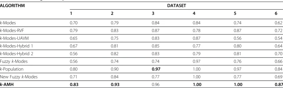
Table 2 Clustering accuracy scores for all datasets

ALGORITHM DATASET

1 2 3 4 5 6

k-Modes 0.70 0.79 0.84 0.84 0.74 0.62

k-Modes-RVF 0.79 0.83 0.87 0.78 0.87 0.72

k-Modes-UAVM 0.65 0.75 0.83 0.87 0.56 0.54

k-Modes-Hybrid 1 0.67 0.81 0.85 0.77 0.80 0.64

k-Modes-Hybrid 2 0.56 0.82 0.83 0.79 0.81 0.70

Fuzzyk-Modes 0.56 0.74 0.74 0.97 0.76 0.66

k-Population 0.80 0.90 0.97 1.00 0.97 0.84

New Fuzzyk-Modes 0.71 0.84 0.77 1.00 0.77 0.69

where k is the number of clusters, a

is the

num-ber of instances occurring in both cluster i and its

corresponding haplogroup or surname, and n is

the number of instances in the dataset.

Clustering performance

Table 2 shows the clustering accuracy scores for all data-sets (boldface indicates the highest clustering accuracy). Based on these results, the performance of the k-AMH algorithm was very promising. Out of six datasets, our algorithm obtained the highest clustering accuracy scores for datasets 1, 2, 4, 5, and 6. In fact, the algorithm also achieved the optimal clustering accuracy for two datasets (4 and 5). However, for dataset 3, the results show that the accuracy of the k-AMH algorithm was 0.01 lower than that of the k-Population algorithm. A statistical t-test was carried out for further verification. This indicated thatt(101.39) = 0.65, andp= 0.51. Thus, there was no significant difference at the 5% level be-tween the accuracy score of our k-AMH algorithm and the k-Population algorithm. This means that both algo-rithms displayed an equal performance for this dataset.

During the experiments, thek-AMH algorithm did not encounter any difficulties. However, the Fuzzy k-Modes

and the New Fuzzyk-Modes algorithms faced problems with datasets 1, 5, and 6. For dataset 1, the problem was caused by the extreme number of objects in Class R (475), which covered about 63% of the total objects. Fur-ther, for datasets 5 and 6, the problem was caused by many similar objects in a larger number of classes. In particular, both algorithms faced the problemP2caused

by the initial centroid selections. Note also that the results for both algorithms were based on the diverse method, an initial centroid selection proposed by Huang [25].

For an overall comparison, Table 3 shows the results of all Y-STR datasets. It clearly indicates that the k-AMH algorithm obtained the highest accuracy score of 0.93. The closest score of 0.91 belongs to the k-Population algo-rithm. Furthermore, thek-AMH algorithm also recorded the best results in terms of standard deviation (0.07), the lower bound (0.93), the upper bound (0.94), and the mini-mum accuracy score (0.79).

For further verification, a one-way ANOVA test was carried out. This indicated that the assumption of homogeneity of variance was violated; therefore, the Welch F-ratio is reported. There was a significant vari-ance in the clustering accuracy scores among the Table 3 Clustering accuracy scores for all Y-STR datasets

N Mean Std. Dev. 95% Confidence Interval for Mean Min Max

Lower Bound Upper Bound

k-Mode 600 0.76 0.13 0.75 0.77 0.45 1.00

k-Mode-RVF 600 0.81 0.11 0.80 0.82 0.56 1.00

k-Mode-UAVM 600 0.70 0.17 0.69 0.71 0.38 1.00

k-Mode-Hybrid 1 600 0.76 0.13 0.75 0.77 0.38 1.00

k-Mode-Hybrid 2 600 0.75 0.14 0.74 0.76 0.45 1.00

Fuzzyk-Mode 600 0.74 0.16 0.73 0.75 0.32 1.00

k-Population 600 0.91 0.09 0.91 0.92 0.59 1.00

New Fuzzyk-Mode 600 0.80 0.13 0.79 0.81 0.44 1.00

k-AMH 600 0.93 0.07 0.93 0.94 0.79 1.00

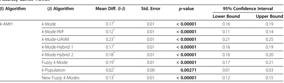
Table 4 Multiple comparisons for thek-AMH algorithm

Accuracy Games–Howell

(I) Algorithm (J) Algorithm Mean Diff. (I-J) Std. Error p-value 95% Confidence Interval

Lower Bound Upper Bound

k-AMH k-Mode 0.17* 0.01 < 0.00001 0.16 0.19

k-Mode-RVF 0.12* 0.01 < 0.00001 0.11 0.14

k-Mode-UAVM 0.23* _{0.01 < 0.00001 0.21 0.25}

k-Mode-Hybrid 1 0.17* _{0.01 < 0.00001 0.16 0.19}

k-Mode-Hybrid 2 0.18* 0.01 < 0.00001 0.16 0.20

Fuzzyk-Mode 0.19* _{0.01 < 0.00001 0.17 0.21}

k-Population 0.02* _{0.00 0.00271 0.01 0.03}

New Fuzzyk-Modes 0.13* 0.01 < 0.00001 0.12 0.15

nine algorithms, in which F(8, 2230) = 378, p < 0.001, and ω2= 0.25. Thus, the Games–Howell procedure was used for a multiple comparison among the nine algo-rithms. Table 4 shows the result of this comparison with regard to the k-AMH algorithm against the other eight algorithms. At the 5% level of significance, it is clearly shown that the k-AMH algorithm (M = 0.93, 95% CI [0.93, 0.94]) differed from the other eight algorithms (allP values < 0.001). Thus, the performance ofk-AMH algorithm exhibited a very significant difference com-pared to the other algorithms.

Efficiency

We now consider the time efficiency of thek-AMH algo-rithm. The computational cost of the algorithm depends on the nested loop for k(n-k), where k is the number of clusters andnis the number of data required to obtain the cost function,P(À). The functionP(À)involves the num-ber of attributes m in calculating the distances and the membership values for its partition matrix wli. Thus, the

overall time complexity isO(km(n-k)). However, the time efficiency of the k-AMH algorithm will not reach O(n2) because the value ofkin the outer loop will not become

equivalent to the value of n-k in the inner loop. See pseudo-code for a detailed implementation of these loops.

A scalability test was also carried out for the k-AMH algorithm. These experiments were based on a dataset called Connect [42]. This dataset consisted of 65,000 data, 42 attributes, and three classes. Two scalability tests were conducted: (a) scalability against the number of objects, when the number of clusters was three, and (b) scalability against the number of clusters, when the number of objects was 65,000. The test was performed on a personal computer with an Intel® Core™ 2 DUO Processor with 2.93 GHz and 2.00 GB memory. Figure 5 (a) and (b) illustrate the results of the tests. In conclu-sion, the runtime of the k-AMH algorithm increased linearly with the number of clusters and data.

Conclusions

Our experimental results indicate that the performance of the proposed k-AMH algorithm for partitioning Y-STR data was significantly better than that of the other algo-rithms. Our algorithm handled all problems, as described previously, and was not too sensitive toP0, the initial

cen-troid selection, even though the datasets contained a lot of similar objects. Moreover, the concept of P2in using the

object (the data itself) as the approximate center of a clus-ter has significantly improved the overall performance of the algorithm. In fact, our algorithm is the most consistent of those tested because the difference between the mini-mum and maximini-mum scores is smaller. Thek-AMH algo-rithm always produces the highest minimum score for each dataset. In conclusion, thek-AMH algorithm is an ef-ficient method of partitioning Y-STR categorical data.

Competing interests

The authors declare that they have no competing interests.

Authors' contributions

AS carried out the algorithm development and experiments. ZAB verified the algorithm and the results. MNI verified the Y-STR data and also the results. All authors read and approved the final manuscript.

Acknowledgements

This research is supported by Fundamental Research Grant Scheme, Ministry of Higher Eduction Malaysia. We would like to thank RMI, UiTM for their support for this research. We extend our gratitude to many contributors toward the completion of this paper, including Prof. Dr. Daud Mohamed, En. Azizian Mohd Sapawi, Puan Nuru'l-'Izzah Othman, Puan Ida Rosmini, and our research assistants: Syahrul, Azhari, Kamal, Hasmarina, Nurin, Soleha, Mastura, Fadzila, Suhaida, and Shukriah.

Author details

1_{Center for Computer Sciences, Faculty of Computer and Mathematical}

Sciences, Universiti Teknologi MARA (UiTM), 40450 Shah Alam, Selangor, Malaysia.2_{Medical Faculty, Masterskill University College of Health Sciences,} No. 6, Jalan Lembah, Bandar Seri Alam 81750 Johor Bahru, Johor, Malaysia.

Received: 1 March 2012 Accepted: 22 September 2012 Published: 6 October 2012

References

1. Kayser M, Kittler R, Erler A, Hedman M, Lee AC, Mohyuddin A, Mehdi SQ, Rosser Z, Stoneking M, Jobling MA, Sajantila A, Tyler-Smith C:A comprehensive survey of human Y-chromosomal microsatellites.Am J Hum Genet2004,74(6):1183–1197.

2. Perego UA, Turner A, Ekins JE, Woodward SR:The science of molecular genealogy.National Genealogical Society Quarterly2005,93(4):245–259. 3. Perego UA:The power of DNA: Discovering lost and hidden relationships. Oslo:

World Library and Information Congress: 71st IFLA General Conference and Council Oslo; 2005.

4. Hutchison LAD, Myres NM, Woodward S:Growing the family tree: The power of DNA in reconstructing family relationships.Proceedings of the First Symposium on Bioinformatics and Biotechnology (BIOT-04)2004, 1:42–49.

5. Dekairelle AF, Hoste B:Application of a Y-STR-pentaplex PCR (DYS19, DYS389I and II, DYS390 and DYS393) to sexual assault cases.Forensic Sci Int2001,118:122–125.

6. Rolf B, Keil W, Brinkmann B, Roewer L, Fimmers R:Paternity testing using Y-STR haplotypes: Assigning a probability for paternity in cases of mutations.Int J Legal Med2001,115:12–15.

7. Dettlaff-Kakol A, Pawlowski R:First polish DNA“manhunt”- an application of Y-chromosome STRs.Int J Legal Med2002,116:289–291.

8. Stix G:Traces of the distant past.Sci Am2008,299:56–63. 9. Gerstenberger J, Hummel S, Schultes T, Häck B, Herrmann B:

Reconstruction of a historical genealogy by means of STR analysis and Y-haplotyping of ancient DNA.Eur J Hum Genet1999,7:469–477. 10. International Society of Genetic Genealogy. http://www.isogg.org. 11. The Y Chromosome Consortium. http://ycc.biosci.arizona.edu. 12. Schlecht J, Kaplan ME, Barnard K, Karafet T, Hammer MF, Merchant NC:

Machine-learning approaches for classifying haplogroup from Y chromosome STR data.PLoS Comput Biol2008,4(6):e1000093. 13. Seman A, Abu Bakar Z, Mohd Sapawi A:Centre-based clustering for

Y-Short Tandem Repeats (Y-STR) as Numerical and Categorical data.Proc. 2010 Int. Conf. on Information Retrieval and Knowledge Management (CAMP’10)2010,1:28–33. Shah Alam, Malaysia.

14. Seman A, Abu Bakar Z, Mohd Sapawi A:Centre-Based Hard and Soft Clustering Approaches for Y-STR Data.Journal of Genetic Genealogy2010, 6(1):1–9. Available online: www.jogg.info.

15. Seman A, Abu Bakar Z, Mohd Sapawi A:Attribute Value Weighting in K-Modes Clustering for Y-Short Tandem Repeats (Y-STR) Surname.Proc. of Int. Symposium on Information Technology 2010 (ITsim’10)2010,3:1531– 1536. Kuala Lumpur, Malaysia.

16. Seman A, Abu Bakar Z, Mohd Sapawi A:Hard and Soft Updating Centroids for Clustering Y-Short Tandem Repeats (Y-STR) Data.Proc. 2010 IEEE Conference on Open Systems (ICOS 2010)2010,1:6–11. Kuala Lumpur, Malaysia.

17. Seman A, Abu Bakar Z, Mohd Sapawi A:Modeling Centre-based Hard and Soft Clustering for Y Chromosome Short Tandem Repeats (Y-‐STR) Data. Proc. 2010 International Conference on Science and Social Research (CSSR 2010)2010,1:73–78. Kuala Lumpur, Malaysia.

18. Seman A, Abu Bakar Z, Mohd Sapawi A:Centre-based Hard Clustering Algorithm for Y-STR Data.Malaysia Journal of Computing2010,1:62–73. 19. Seman A, Abu Bakar Z, Isa MN:Evaluation of k-Mode-type Algorithms for

Clustering Y-Short Tandem Repeats.Journal of Trends in Bioinformatics 2012,5(2):47–52.

20. Ng M, Jing L:A new fuzzy k-modes clustering algorithm for categorical data.International Journal of Granular Computing, Rough Sets and Intelligent Systems2009,1(1):105–119.

21. He Z, Xu X, Deng S:Attribute value weighting in k-Modes clustering. Ithaca, NY, USA: Cornell University Library, Cornell University; 2007:1_–15. available online: http://arxiv.org/abs/cs/0701013v1.

22. Ng MK, Junjie M, Joshua L, Huang Z, He Z:On the impact of dissimilarity measure in k-modes clustering algorithm.IEEE Trans Pattern Anal Mach Intell2007,29(3):503–507.

23. Kim DW, Lee YK, Lee D, Lee KH:k-Populations algorithm for clustering categorical data.Pattern Recogn2005,38:1131–1134.

24. Huang Z, Ng M:A Fuzzy k-Modes algorithm for clustering categorical data.IEEE Trans Fuzzy Syst1999,7(4):446_–452.

26. MacQueen JB:Some methods for classification and analysis of multivariate observations.The 5th Berkeley Symposium on Mathematical Statistics and Probability1967,1:281–297.

27. Ralambondrainy H:A conceptual version of the k-Means algorithm. Pattern Recogn Lett1995,16:1147–1157.

28. Bobrowski L, Bezdek JC:c-Means clustering with the l1 and l∞norms. IEEE Trans Syst Man Cybern1989,21(3):545–554.

29. Salim SZ, Ismail MA:k-Means-type algorithms: A generalized convergence theorem and characterization of local optimality.IEEE Trans Pattern Anal Mach Intell1984,6:81–87.

30. WorldFamilies.net. http://www.worldfamilies.net.

31. Fitzpatrick C:Forensic genealogy. Fountain Valley: Cal.: Rice Book Press; 2005. 32. Ireland yDNA project. www.familytreedna.com/public/IrelandHeritage/. 33. Finland DNA Project. http://www.familytreedna.com/public/Finland/. 34. Y-Haplogroup project. www.worldfamilies.net/yhapprojects/. 35. Clan Donald Genealogy Project. http://dna-project.clan-donald-usa.org. 36. Flannery Clan. http://www.flanneryclan.ie.

37. Doug and Joan Mumma’s Home Page. http://www.mumma.org. 38. Williams Genealogy. http://williams.genealogy.fm.

39. Phillips DNA Project.http://www.phillipsdnaproject.com. 40. Brown Genealogy Society. http://brownsociety.org.

41. San OM, Huynh V, Nakamori Y:An alternative extension of the K-Means Algorithm for clustering categorical data.IJAMCS2004,14(2):241–247. 42. Blake CL, Merz CJ:UCI repository of machine learning database. 1989.

doi:10.1186/1756-0500-5-557

Cite this article as:Semanet al.:An efficient clustering algorithm for

partitioning Y-short tandem repeats data.BMC Research Notes2012

5:2101791285670500.

Submit your next manuscript to BioMed Central and take full advantage of:

• Convenient online submission

• Thorough peer review

• No space constraints or color figure charges

• Immediate publication on acceptance

• Inclusion in PubMed, CAS, Scopus and Google Scholar

• Research which is freely available for redistribution