Implementation of Fuzzy Based Flow Controller using VHDL

(1)

International Journal of Innovative Technology and Exploring Engineering (IJITEE) ISSN: 2278-3075, Volume-8 Issue-8, June, 2019



Abstract: The flow control is an essential process in a plant. The fuzzy based controller can be used in controlling the flow of liquid applications effectively. The flow rate of liquid can be controlled by opening and closing of valve. Fuzzy inference system to control the flow rate was developed and proved that it’s response is better than PID controller. It is always challenging to implement a fuzzy controller. This paper discusses about the development of VHDL code for the implementation of fuzzy logic based flow controller in FPGA. In this paper the VHDL code is developed for evaluating the degree of membership function of crisp input, finding minimum-maxima for defuzzification. The simulation results of VHDL model matches with the simulation results of fuzzy controller developed using fuzzy toolbox of MATLAB® version 7.11.0.584 (R2020b). Matlab. Finally the VHDL code can be used for implementing the fuzzy flow rate controller in FPGA. The developed fuzzy controller can be used for controlling the flow rate effectively. The fuzzy based flow controller is developed using VHDL language and simulated by using Xilinx ISE 14.5 version.

Index Terms: fuzzy logic, flow rate, FPGA, VHDL, fuzzification

I. INTRODUCTION

Measuring and controlling flow rate in process plants presents challenges of its own. Both gas and liquid flow can be measured in volumetric or mass flow rates, such as litres per second or kilograms per second. These measurements can be converted between one another if the fluid density is known. The density for a liquid is almost independent of the liquid conditions; however, this is not the case for gas, the density of which depends greatly upon pressure, temperature and to a lesser extent, the gas composition. With so many different variables that could affect flow rate, flow measurement and control is susceptible to disturbances. Because of this, flow controllers need to be robust to optimize the performance of a plant. Fuzzy logic based flow rate controller has been proposed to replace the conventional PID controller due to its superior applicability and robustness [1]. The main objective of this paper is to develop the VHDL code to implement the fuzzy logic based flow controller in FPGA.

A. Introduction to fuzzy logic

Fuzzy logic is a form of many-valued logic in which the truth values of variables may be any real number between 0 and 1 inclusive. It is employed to handle the

Revised Manuscript Received on June 05, 2019

Dr. Yogesh, Department of Electronics and Communication Engineering, GMR Institute of Technology, Rajam, Andhra Pradesh, India.

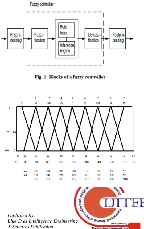
concept of partial truth, where the truth value may range between completely true and completely false.By contrast, in Boolean logic, the truth values of variables may only be the integer values 0 or 1. The term fuzzy logic was introduced with the 1965 proposal of fuzzy set theory by Lotfi Zadeh [2]. There are specific components characteristic of a fuzzy controller to support a design procedure. Controls of processes through fuzzy logic have been demonstrated in 1974 by E.H Mamdani and S. Assilian [3]. The fuzzy if/then rules were used to regulate a model steam engine; and with that a great number of fuzzy control applications have been deployed. The block diagram of fuzzy controller is shown in Fig. 1. The fuzzification is the process of mapping crisp input into corresponding fuzzy memberships. It takes input values and determines the degree to which they belong to each of the fuzzy sets via membership functions. The inference engine defines mapping from input fuzzy sets into output fuzzy sets. It determines the degree to which the antecedent is satisfied for each rule. If the antecedent of a given rule has more than one clause, fuzzy operators are applied to obtain one number that represents the result of the antecedent for that rule. It is possible that one or more rules may fire at the same time. Outputs for all rules are then aggregated.

During aggregation, fuzzy sets that represent the output of each rule are combined into a single fuzzy set. Fuzzy rules are fired in parallel, which is one of the important aspects of an FIS. In an FIS, the order in which rules are fired does not affect the output. The defuzzifier maps output fuzzy sets into a crisp number. The most popular defuzzification method is the centroid, which calculates and returns the center of gravity of the aggregated fuzzy set [4], [5] and [6].

B. Introduction to VHDL and FPGA

The VHDL models are simulated, synthesized and finally implemented in FPGAs [7]. VHDL is one of the most accepted and widely used languages for describing digital system. VHDL has been approved by IEEE as a standard language for designing hardware. In 1987 standard version of VHDL “IEEE Std 1076-1987” was launched for industrial use. In 1993 language was upgraded with new features and upgraded version “IEEE Std 1076-1993” was launched [7]. Subsequently, many computers – aided engineering companies put lot of efforts into developing tools based on VHDL.

Implementation of Fuzzy Based Flow Controller

using VHDL

(2)

At this point of time VHDL is supported by nearly all design automation tools and is widely used in the design cycle for Simulation, Synthesis and Testing. The most important part of VHDL is its technology independency [7] and [8]. After writing the VHDL model of a design the simulation is carried out. The functionality of the controller is verified from the waveform generated by the simulation tool. Once the VHDL model is simulated then it passes through synthesis tool. Synthesis tool reads the VHDL description. If no syntax and synthesis error exists then synthesizer produces an output net list in Electronic Design Intermediate Format (EDIF) for the target technology. The Synthesis creates a design that implements the required functionality and makes the designer’s constraints in speed, area or power. The Place And Route (PAR) tool is used to take the design net list and implement it in the target technology. Input to Place tool are net list and timing constraints and it places each primitive from the net list to appropriate location on target technology. Route tool connect the primitives according to net list and output of the PAR tool is bit map file / Graphic Design System-II (GDS-II) which is used to implement design in FPGA / Application Specific Integrated Circuit (ASIC) [9]. In antifuse FPGA bit map file is used to burn the appropriate fuses and implement the required functionality required whereas in reprogrammable FPGA this file is used to turn on appropriate transistors [7] and [8]. FPGA was invented in 1984 by Ross Freeman, Xilinx co-founder [7]. FPGA is different from earlier versions of Programmable Logic Devices (PLDs) because it does not contains array of AND-OR planes rather it contains a two dimensional array of Configurable Logic Blocks (CLBs). The basic element inside CLBs where the logic is stored is Look-Up Tables (LUTs). A typical CLB contains four/five input LUTs [9]. After generating the bit map file with the help of place and route tool it is downloaded in FPGA to reconfigure it. The FPGA can be programmed according to our requirements by using VHDL.

II. FUZZYBASEDFLOWCONTROLLER

A fuzzy inference system was developed for flow control application using Mamdani approach [1]. The Fuzzy Logic Toolbox in MATLAB was used to develop the fuzzy inference system to control the flow of liquid in the plant. The controller has two inputs i.e. the error, E and the rate of change of flow which is,delPV. The output is the control signals to the control valve, hence the manipulated variable mv. The inputs, E and delPV and the output mv each has nine membership functions; negative large (NL), negative intermediate (NI) negative medium (NM), negative small (NS), zero (Z), positive small (PS), positive medium (PM), positive intermediate (PI) and positive large (PL). The membership functions of input variable error and delPV are shown in Fig. 2 and Fig. 3 respectively. The rule base is developed using eighty one rules and shown in Table I. The range of the input ‘error’ is from [-50 50] because the range of flow of liquid for this application is set from 15l/min

to 45l/min. The range of second input delPV is [-20 20]. The range of manipulating variable is [-0.15 0.15].

III. DEVELOPMENTPROCESSOFFUZZYFLOW

CONTROLLERUSINGVHDL

The input data from the real world is called as crisp value. The crisp value from the real world is first converted into fuzzy value and this process is called fuzzification. The fuzzification is done by the fuzzifier block of fuzzy controller. The output of fuzzifier is feed to the rule base block. Depending upon the inputs and the developed rule base an output in the form of fuzzy value is generated. The fuzzy value generated by rule base is of no use for real world therefore it has to be converted back in crisp form and this process is called defuzzification. The defuzzification is done by the defuzzifier block of fuzzy controller.

A. Implementation of Fuzzification Algorithm in VHDL

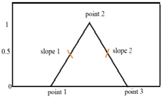
In fuzzy logic each value is represented in the form of membership function with the value in the range (0 to 1). The triangular membership function graph is shown in Fig. 4. It contains three points Point-1, Point-2 and Point-3. The two slopes of two lines on membership graph are represented by Slope-1 and Slope-2 and they are calculated from (1) and (2) as follows [10]:

Slope-1 = (y2 - y1) ÷ (Point-2 – Point-1) (1) Slope-2 = (y2 - y1) ÷ (Point-3 – Point-2) (2) Where y2 is 1 (FFH) maximum value of a membership function and y1 is 0 (00H) minimum value of a membership function.

The degree of membership of any value on x-axis less than or equal to the value of Point 1 and greater than or equal to the value of Point 3 is always 0. The degree of membership of any value on x-axis greater than the value of Point 1 and less than Point-2 is calculated by using (3) as follows [10]:

µ = (Input Value – Point-1) × Slope-1 (3) The degree of membership of any value on x-axis greater than or equal to the value of Point-2 and less than Point-3 is calculated by using (4) as follows:

µ = 1- (Input Value – Point-2) × Slope-2 (4) The notations used in representing a point in a membership function graph are as follows [10]:

P represents the point, 1st digit represents number of point (i.e. Point-1, Point-2 or Point-3) of membership function graph and 2nd digit represents the number of linguistic variable.

(3)

If the input value intersects only with one linguistic variable then it has only one finite degree of membership of the intersected linguistic variable and for the remaining linguistic variables it’s degree of membership is zero. If the input value intersects with two linguistic variables then it has two finite degree of membership of the intersected linguistic variables and for the remaining linguistic variables it’s degree of membership is zero. The crisp data of two variables are fuzzified as follows:

i. Fuzzification of Error - Input parameter ‘ERROR’ is

fuzzified in to nine linguistic variables. The universe of discourse of nine linguistic variables of input parameter ‘ERROR’ is represented in figure 1. The linguist variable NL (Negative Large), NI (Negative Intermediate), NM (Negative Medium), NS (Negative Small), Z (Zero), PS (Positive Small), PM (Positive Medium), PI (Positive Intermediate), PL (Positive Large), are designated as 1, 2, 3, 4, 5, 6, 7, 8, and 9. For instance Point-3 of linguistic variable NL is represented by P31, Point-2 of linguistic variable PS is represented by P26 and Point-1 of linguistic variable is represented by P19. The x-axis represents the universe of discourse of variation of cane weight from and it is from -50l/min to 50l/min. The universe of discourse of variation of cane weigh is represented from (00H to FFH) in digital form.

The slope for the linguistic variables of Input Parameter ‘ERROR’ are calculated as follows:

(i) Calculation of Slopes of Linguistic Variable NL Slope-2NL- Point-2 and Point-3 of NL is represented by P21

and P31 respectively and it’s Slope-2 is calculated from (2) as follows:

Slope-2NL = [(FFH – 00H) / (P31 - P21)] = [FFH / (14H –

0AH)] = 19H

(ii) Calculation of Slopes of Linguistic Variable NI (a) Slope-1NI – Point-1 and Point-2 of NI is represented by

P12 and P22 respectively and it’s Slope-1 is calculated from (1) as follows:

Slope-1NI = [(FFH – 00H) / (P22 – P12)] = [FFH / (14H –

0AH)] = 19H

(b) Slope-2NI – Point-3 of NI is represented by P32 and its

Slope-2 is calculated from (2) as follows:

Slope 2NI = [(FFH – 00H) / (P32 – P22)] = [FFH / (1EH –

14H)] = 19H

(iii) Calculation of Slopes of Linguistic Variable NM (a) Slope-1NM–Point-1 and Point-2 of NM is represented by

Slope-1NM = [(FFH – 00H) / (P23 – P13)] = [FFH / (1EH –

14H)] = 19H

(b) Slope-2NM – Point-3 of NM is represented by P33 and its

Slope 2EL = [(FFH – 00H) / (P33 – P23)] = [FFH / (28H –

1EH)] = 19H

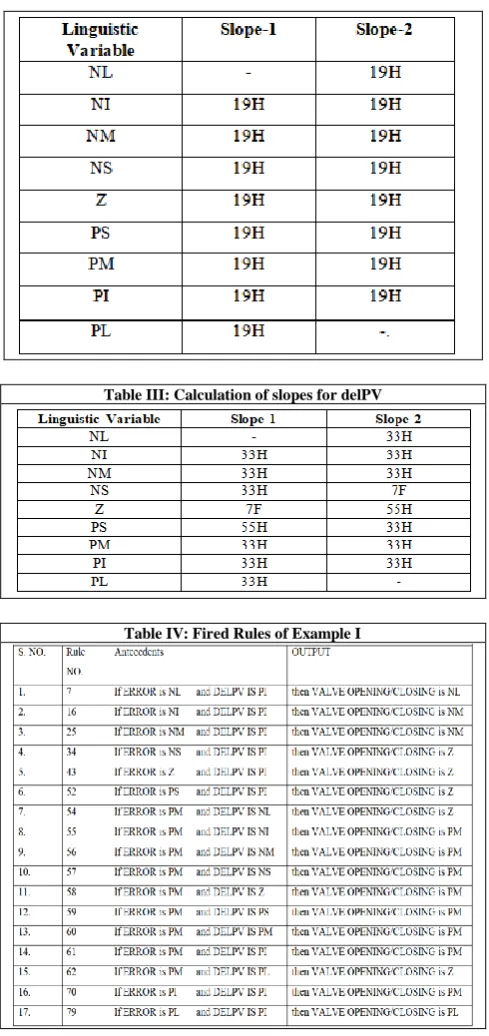
Slopes for all the linguistic variables of input parameter ERROR are calculated as explained above and represented in Table II.

ii. Fuzzification of delPV - The universe of discourse of seven linguistic variables of input parameter ‘delPV’ is

represented in figure 2. The linguistic variable NL

(NEGATIVE LARGE), NI (NEGATIVE

INTERMEDIATE), NM (NEGATIVE MEDIUM), NS (NEGATIVE SMALL), Z (ZERO), PS (POSITIVE SMALL), PM (POSITIVE MEDIUM), PI (POSITIVE INTERMEDIATE) and PL (POSITIVE LARGE) are designated as 1, 2, 3, 4, 5, 6,7,8and 9. The x-axis point represents the universe of discourse of variation of delPV, a range of [-20 20] is chosen. The universe of discourse of variation of rate of change of flow is represented from (00 to 28H) in digital form.

The slope for the linguistic variables of Input Parameter ‘delPV’ are calculated as follows:

(i) Calculation of Slopes of Linguistic Variable NL Slope-2NL- Point-2 and Point-3 of NL is represented by P21

and P31 respectively andit’s Slope-2 is calculated from (2) as follows:

Slope-2NL = [(FFH – 00H) / (P31 - P21)] = [FFH / (08H –

03H)] = 33H

(ii) Calculation of Slopes of Linguistic Variable NI (a) Slope-1NI – Point-1 and Point-2 of NI is represented by

Slope-1NI = [(FFH – 00H) / (P22 – P12)] = [FFH / (08H

– 03H)] = 33H

(b) Slope-2NI – Point-3 of NI is represented by P32 and its

Slope 2NI = [(FFH – 00H) / (P32 – P22)] = [FFH / (0DH

– 08H)] = 33H

(iii) Calculation of Slopes of Linguistic Variable NM (a) Slope-1NM–Point-1 and Point-2 of NM is represented by

Slope-1NM = [(FFH – 00H) / (P23 – P13)] = [FFH /

(0DH – 08H)] = 33H

(b) Slope-2NM – Point-3 of NM is represented by P33 and its

Slope 2EL = [(FFH – 00H) / (P33 – P23)] = [FFH / (12H

– 0DH)] = 33H

Slopes for all the linguistic variables of input parameter delPV are calculated as explained above and represented in Table III.

B. Calculation of Degree of Membership of ‘ERROR’

If the error is 25l/min and it is represented as 4BH in hexadecimal. The 4BH value will intersects linguistic variables PM and PI of ‘ERROR’. The degree of membership of this input value for linguistic variable PM is calculated from (4) as follows:

= 1- (Input

= FFH-(4BH-46H)*19H =82H=130D

The degree of membership of this input value for linguistic variable PI is calculated from (3) as follows:

=(Input

(4)

The degree of membership function of error of 25 l/min in seven linguistic variables is zero and it is given below for all nine linguistic variables of input parameter ‘ERROR’:

=7DH, =82H and = = = = = =

= 0.

The part of VHDL code used for the fuzzification of input parameter ‘ERROR’ is shown in Fig. 5 and the simulation result showing the membership of linguistic variable PM and PI when ERROR is 25 l/min is shown in Fig. 6.

C. Calculation of Degree of membership of ‘delPV’

If the rate of change of flow is 12.5l/min and it is represented as 21H in hexadecimal. The 21H value will intersects linguistic variable PI of ‘delPV’. The degree of membership of this input value for linguistic variable PI is calculated from (4) as follows:

= 1 – (Input Value – P28) * 0H = FF – (21H – 21H) * 0 = FFH

The degree of membership function of rate of change of flow of 12.5 l/min in nine linguistic variables is zero and it is given below for all nine linguistic variables of input parameter ‘delPV’:

=FFH, = = = = = = = = 0

The part of VHDL code used for the fuzzification of input parameter ‘delPV’’ is shown in Fig. 7 and the simulation result showing the membership of linguistic variable PI when delPV is 12.5l/min is shown in Fig. 8.

D. Implementation of Rule Inference Algorithm in VHDL

The flow controller designed using MATLAB has 81 rules as shown in Table I. The Rule-1, for instance, is “If ERROR is PM and delPV is PI then valve opening/closing is PM”. The value of minimum degree of membership among the two antecedents will be the consequent and we represent it as Min (R1). The consequents of all 81 rules will be computed. If more than one rule is fired for same linguistic variable of output parameter, then maximum value of consequent of all the fired rules will be the fuzzy output of corresponding linguistic variable.

In continuation with previous example, the error of 25l/min has degree of membership in PM and PI linguistic variables of input parameter ‘ERROR’, the rate of flow of 12.5l/min has degree of membership in PI linguistic variables in input parameter. There are 14 rules having PM and PI linguistic variables in ‘ERROR’, PI linguistic variables in ‘delPV’. All the fired rules are shown in Table IV.

The minimum degree of membership among the two antecedents of all fired rules is as follows:

Min (R61) = 82H Min (R70) = 7DH

The minimum value of all remaining fired rules is 00H. The part of VHDL code used for calculation of Min (R0) to Min (R79) is shown in Fig. 8 and the simulation result showing the values of Min (R0) to Min (R79) for error 25l/min is shown in Fig. 9.

The output parameter of fuzzy controller is ‘OUTPUT’ and it has nine linguistic variables NL, NI, NM, NS, Z, PS, PM, PI and PL. There are nine rules involving NL as output, five rules involving NI as output, eleven rules involving NM as

output, six rules involving NS as output, seventeen rules involving Z as output, eight rules involving PS as output, eleven rules involving PM as output, five rules involving PI as output and nine rules involving PL as output. The rules involving the nine linguistic variables of ‘OUTPUT’ are shown in Table 3.4.

In continuation with previous example, there are one rule involving NL as output linguistic variable, zero rules involving NI as output linguistic variable, two rules involving NM as output linguistic variable, zero rules involving NS as output linguistic variable, five rules involving Z as output linguistic variable, zero rules involving PS as output linguistic variable, eight rules involving PM as output linguistic variable, zero rules involving PI as output linguistic variable and one rule involving PL as output linguistic variable. The fired rules involving the nine linguistic variables of ‘OUTPUT’ for Example-I are shown in Table 3.5.

The maximum value of consequents among all the fired rules having same output linguistic variable is chosen as the final fuzzy value of corresponding linguistic variable. By combing the maximum-minimum operation final fuzzy value of all linguistic variables of output parameter is calculated. The final value of NL is represented by MaxR (0), NI by MaxR (1), NM by MaxR (2), NS by MaxR (3), Z by MaxR (4), PS by MaxR (5), PM by MaxR (6), PI by MaxR (7) and PL by MaxR (8).

The fuzzy output of all linguistic variables of output parameter ‘SPEED’ of Example- I is calculates as follows: MaxR(0)=maximun[min(R0),min(R1),min(R2),min(R3),m in(R4),min(R5),min(R6),min(R7),min(R8)]

MaxR(1)=maximum[(min(R12),min(R13),min(R14), min(R30),min(R32)]

MaxR(2)=maximum(min(R9),min(R10),min(R16),min(R1 7),min(R19),min(R20),min(R21),min(R22), min(R23) , min(R24), min(R25)] MaxR(3)=maximum[(minR(11),minR(15),minR(29),minR (31),minR(33), minR(45)] MaxR(4)=maximum[(minR(18),minR(26),minR(28),minR (34),minR(36),minR(37),minR(38),minR(39),minR(40),mi nR(41),minR(42),minR(43),minR(44),minR(46),minR(52), minR(54),minR(62)] MaxR(5)=maximum[(minR(27),minR(35),minR(47),minR (49),minR(51),minR(53),minR(65),minR(69)] MaxR(6)=maximum[(minR(55),minR(56),minR(57),minR (58),minR(59),minR(60),minR(61),minR(63),minR(64) , minR(70), minR(71)]

MaxR(7)=maximum [(minR(48),minR(50),minR(66),

minR(67), minR(68)]

(5)

The computed value of MaxR (0)=00H, MaxR (1) = 00H, MaxR (2)=00H, MaxR (3)=00H, MaxR (4)=00H, MaxR (5)=87H, MaxR (6)=7DH, MaxR (7)=82H and MaxR (8)=00H.

The part of VHDL code used for the calculation of maximum value of all linguistic variables of output parameter ‘OUTPUT’ and the simulation result shown in Fig. 9 and Fig. 10 respectively.

E. Implementation of Defuzzification in VHDL

Defuzzification forms the last and an important step in designing a fuzzy system. Defuzzified values generate a single crisp value, which is OPENING/CLOSING of the valve. The Sugeno method of defuzzification is used and in this method, we multiply the fuzzy output obtained from aggregation with its corresponding singleton value, then divide the sum of these values by the sum of all the fuzzy output obtained from the rule evaluation—that is, the values obtained after aggregation.

After calculating the fuzzy output of all linguistic variables of output parameter there is a need to combine them to generate a crisp output which can be utilized for control action. This process of conversion of fuzzy output into crisp value is called as defuzzification. Although Mamdani style of fuzzy logic is widely used because of its resemblance with human thinking but its implementation is not computational efficient. The Sugeno style of fuzzy logic is more suitable for the implementation because output in Sugeno style require a singleton value. The singleton values of all linguistic variables of output parameter ‘OUTPUT’ are as follows : Singleton value of linguistic variable NL=SNL=03H Singleton value of linguistic variable NI=SNI=06H Singleton value of linguistic variable NM=SNM=09H Singleton value of linguistic variable NS=SNS=0CH Singleton value of linguistic variable Z=SZ= 0FH Singleton value of linguistic variable PS=SPS=12H Singleton value of linguistic variable PM=SPM=15H Singleton value of linguistic variable PI=SPI =18H Singleton value of linguistic variable PL=SPL=1BH The weighted average method is used during defuzzification in Sugeno style of fuzzy logic. The crisp (defuzzified) output is obtained by (5) as follows:

Crispoutput = (Numerator) / (Denominator) (5) Here, Numerator = [{MaxR (0) × SEL} + {MaxR (1) × SVL} + {MaxR (2) × SL} + {MaxR (3) × SJR} + {MaxR (4) × SH} + {MaxR (5) × SVH} + {MaxR (6) × SHE} + {MaxR (7) × SUH} + {MaxR (8) × SSH}

Denominator = MaxR (0) + MaxR (1) + MaxR (2) + MaxR (3) + MaxR (4) + MaxR (5) + MaxR (6) + MaxR (7) + MaxR (8)

In continuation with previous example, Numerator = 1671H

(0001011001110001) and Denominator = 00FFH

(11111111) and = 16H = 22D. The

represents valve opening/closing.

IV. RESULTANDDISCUSSIONS

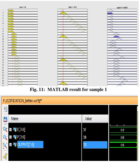
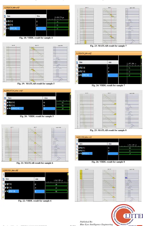
After implementing the above steps, we successfully developed the VHDL code for flow control fuzzy logic using a triangular membership function and centroid defuzzification. We have taken 10 sample inputs and simulated the fuzzy based flow controller developed using fuzzy toolbox of Matlab and VHDL model. The MATLAB simulation result of fuzzy based flow controller of ten samples is shown in Fig. 11, Fig. 13, Fig. 15, Fig. 17, Fig. 19, Fig. 21, Fig. 23, Fig. 25, Fig. 27 and Fig. 29. The VHDL model simulation result of fuzzy flow controller of ten samples are shown in Fig. 12, Fig. 14, Fig. 16, Fig. 18, Fig. 20, Fig. 22, Fig. 24, Fig. 26, Fig. 28 and Fig. 30.

The Comparison between MATLAB and VHDL Simulation of Fuzzy Based Flow Controller is shown in Table V. The VHDL simulation result of manipulating variable of flow controller is very close to MATLAB simulation result.

V. CONCLUSION

[image:5.595.314.548.458.830.2]

The final implementation of fuzzy based flow controller developed using fuzzy toolbox of Matlab software is done VHDL language and simulated by using Xilinx ISE 14.5 version. It is essential that the Matlab results should be sufficiently close to VHDL model. The experimentations results of this paper justify that the VHDL code developed for the fuzzy based flow controller generates result which is nearly equal to Matlab result. I future the VHDL code can be used for the implementation of fuzzy based flow controller in FPGA and the results can be verified in real environment.

(6)

[image:6.595.317.538.55.185.2]

Fig. 2: Fuzzified input parameter ‘ERROR’ with point representation

[image:6.595.64.270.104.242.2]

Fig. 3: Fuzzified input parameter ‘delPV’ with point representation

Fig. 4: Representation of a triangular membership functiongraph

ELSIF(E>=X"46" AND E<X"50”) THEN

DMF_E(0)<=X"0000";

DMF_E(1)<=X"0000";

DMF_E(2)<=X"0000";

DMF_E(3)<=X"0000";

DMF_E(4)<=X"0000";

DMF_E(5)<=X"0000";

DMF_E(6) <=(X"FF")-(E-P27)*X"19";

DMF_E(7)<=(E-P18)*X"19";

DMF_E(8)<=X"0000";

Fig. 5: Part of VHDL code for calculating degree of membership of input variable error

Fig. 6: Degree of membership when Error is 25 l/min = dmf_E_f[6] = 82H, =dmf_E_f[7] = 7DH

ELSIF(P=X"21H")THEN

DMF_P(0)<=X"0000";

DMF_P(1)<=X"0000";

DMF_P(2)<=X"0000";

DMF_P(3)<=X"0000";

DMF_P(4)<=X"0000";

DMF_P(5)<=X"0000";

DMF_P(6) <=X"0000";

DMF_P(7)<=(X"FF")-(P-P28)*X"FF";

[image:6.595.89.256.337.441.2]

DMF_P(8)<=X"0000";

Fig. 7: Part of VHDL code for calculating degree of membership of input variable delPV

Fig. 8: Degree of membership when delPV is 12.5 l/min =dmf_P_f[7] = FFH

PROCESS(DMF_E_,DMF_P_F)

BEGIN

minR(0) <=min(DMF_E_F(0),DMF_ P_F(0));

minR(1) <=min(DMF_E_F(0),DMF_P_F(1));

[image:6.595.315.533.445.569.2]

(7)

[image:7.595.317.547.50.167.2]

Fig. 9: The part of VHDL code for the calculation of maximum value of all linguistic variables of output parameter ‘OUTPUT’

[image:7.595.58.284.183.306.2]

Fig. 10: VHDL Simulation Showing Min (R61) by Row 60, Min (R70) by Row 69

Fig. 11: MATLAB result for sample 1

Fig. 12: VHDL result for sample 1

[image:7.595.57.291.366.638.2]

[image:7.595.311.550.458.828.2]

(8)

[image:8.595.46.544.34.823.2]

(9)

[image:9.595.90.546.37.792.2]

[image:9.595.306.551.45.564.2]

Table I: Rule Matrix of Fuzzy Based Flow Controller

Table II: Calculation of slopes for error

Table III: Calculation of slopes for delPV

Table IV: Fired Rules of Example I

[image:9.595.48.287.61.498.2]

(10)

REFERENCES

1. Development and implementation of Fuzzy Logic Controller for Flow

Control Application, Elangeshwaran Pathmanathan, Rosdiazli Ibrahim - 2010 International Conference on Intelligent and Advanced Systems.

2. Zadeh, L. A. (1983). Commonsense knowledge representation based on

fuzzy logic.

3. Mamdani, E.H., Assilian, S., “An Experiment in Linguistic Synthesis

with a Fuzzy Logic Controller,” International Journal of

Human-Computer Studies, Vol. 51, Issue 2, pages 135 – 147, Aug 1999.

4. Mitsuishi, T., Endou, N. and Sidhama, Y., “The concept of fuzzy set and

membership function and basic properties of fuzzy set operation,” Journal of formalized mathematics, vol. 12, pp 1-6, 2003.

5. Lim, O.P., Ling, T.C. and Phang, K.K., “Development of Fuzzy logic

control system,” Malaysian Journal of Computer Science, vol. 11, pp. 8-14, 1998.

6. Fuzzy Logic Toolbox User's Guide, Mathworks Inc., USA, 2010.

7. Misra, Y., “Understanding VHDL” in Digital System Design using

VHDL, 2nd_{ed., Delhi, India: Dhanpatrai & Sons (P) Ltd., 2008, pp. 1-13.}

8. Bhasker, J., “Model Simulation” in A VHDL Primer, 3rd_{ed., New Jersey,}

Prentice-Hall, 1996, pp.98-106.

9. Brown, S. and Vranesic, Z., “Implementation Technology” in

Fundamentals of Digital Logic with Verilog Design, 1st ed., New York, McGraw-Hill Inc., 2003, pp. 67-147.

10. Vyas, D; Misra, Y and Kamath, H.R; “FPGA-Based Fuzzy Controller

Manages Sugarcane Extraction” Xcell Journal, Fourth Quarter, Issue 94, 2015

AUTHORSPROFILE

Dr. Yogesh Misra has 24 years of industrial and teaching experience and currently working as Professor in Electronics and Communication Engineering Department of GMR Institute of Technology, Rajam, Andhra Pradesh, India. Dr. Misra has worked in U V Instruments (P) Ltd, a sugar mill automation company for many years. He has authored two books and his research interest includes VLSI and Embedded Computing. Dr. Misra is life member of ISTE.