2010
Validation of Tool Mark Comparisons Obtained
Using a Quantitative, Comparative, Statistical
Algorithm
L. Scott Chumbley
Iowa State University, [email protected]
Max D. Morris
Iowa State University, [email protected]
M. James Kreiser
Illinois State Police
Charles Fisher
Iowa State University
Jeremy Craft
Iowa State University
See next page for additional authors
Follow this and additional works at:http://lib.dr.iastate.edu/ameslab_pubs
Part of theApplied Statistics Commons,Engineering Education Commons,Forensic Science and Technology Commons,Longitudinal Data Analysis and Time Series Commons, and theMetallurgy Commons
The complete bibliographic information for this item can be found athttp://lib.dr.iastate.edu/ ameslab_pubs/294. For information on how to cite this item, please visithttp://lib.dr.iastate.edu/ howtocite.html.
Comparative, Statistical Algorithm
Abstract
A statistical analysis and computational algorithm for comparing pairs of tool marks via profilometry data is described. Empirical validation of the method is established through experiments based on tool marks made at selected fixed angles from 50 sequentially manufactured screwdriver tips. Results obtained from three different comparison scenarios are presented and are in agreement with experiential knowledge possessed by practicing examiners. Further comparisons between scores produced by the algorithm and visual assessments of the same tool mark pairs by professional tool mark examiners in a blind study in general show good agreement between the algorithm and human experts. In specific instances where the algorithm had difficulty in assessing a particular comparison pair, results obtained during the collaborative study with professional examiners suggest ways in which algorithm performance may be improved. It is concluded that the addition of contextual information when inputting data into the algorithm should result in better performance.
Keywords
forensic science, tool mark comparison, comparison microscope, screwdriver, statistics, striae, material sciences engineering
Disciplines
Applied Statistics | Engineering Education | Forensic Science and Technology | Longitudinal Data Analysis and Time Series | Metallurgy
Comments
This is the accepted version of the following article: Journal of Forensic Sciences, vol. 55, iss. 4, pg. 953-961, 2010, which has been published in final form athttp://dx.doi.org/10.1111/j.1556-4029.2010.01424.x.
Authors
L. Scott Chumbley, Max D. Morris, M. James Kreiser, Charles Fisher, Jeremy Craft, Lawrence Genalo, Stephen Davis, David Faden, and Julie Kidd
This is the accepted version of the following article: Journal of Forensic Sciences, vol. 55, iss. 4, pg. 953-961, 2010, which has been published in final form at http://dx.doi.org/10.1111/j.1556-4029.2010.01424.x.
Genalo
Validation of Tool mark Comparisons Obtained
Using a Quantitative, Comparative, Statistical Algorithm
Iowa State University, Ames Laboratory
Ames, Iowa
*Illinois State Police, Retired
Springfield, Illinois
ABSTRACT: A statistical analysis and computational algorithm for comparing pairs of tool
marks via profilometry data is described. This analysis is superior to ad hoc comparisons based
on maximized correlation values, described in Faden et al. (2007). Empirical validation of the
method is established through experiments based on tool marks made at selected fixed angles
from fifty sequentially manufactured screwdriver tips that had yet to see use. Further
comparisons between scores produced by the algorithm and visual assessments of the same tool
mark pairs by professional tool mark examiners in a blind study in general shows good
agreement between the algorithm and human experts. In a limited number of cases where the
algorithm had difficulty in assessing a particular comparison pair, results obtained during the
visual assessment and in discussion with professional examiners suggest ways in which
algorithm performance may be further enhanced.
KEYWORDS: forensic science, tool mark comparison, comparison microscope, screwdriver,
In the fifteen years since the 1993 Daubert vs. State of Florida decision, increasing attacks have
been aimed at firearm and tool mark examiners by defense attorneys via motions to exclude
evidence based on expert testimony. Such motions claim that the study of tool marks has no
scientific basis, that error rates are unknown and incalculable, and that comparisons are
subjective and prejudicial. Often persuasive, these motions skillfully blend truth with
unsupported assertions or assumptions in a number of ways. Firstly, the claim that scientific
evidence is lacking in tool mark examinations ignores the numerous studies that have been
conducted, especially in the area of firearms [1-4], to investigate the reproducibility and
durability of markings. These studies have shown time and again that while matching of
cartridges cannot be universally applied to all makes and models of guns using all types of
ammunition, the characteristic markings produced are often quite durable and a high percentage
can be successfully identified using optical microscopy. Secondly, the claims that error rates are
unknown, and that the probability of different guns having identical markings has not been
established, are true. However, it must be understood that establishing error rates and
probabilities in the area of tool marks is fundamentally different than in an area such as genetic
matching involving DNA. When considering genetic matching, all the variables and parameters
of a DNA strand are known and error rates can be calculated with a high degree of accuracy.
This is not the case in tool marks where the variables of force, angle of attack, motion of the tool,
surface finish of the tool, past history of use, etc. are not known or cannot be determined, and the
possibility for variation is always increasing as the population under study continues to increase
and change. For practical purposes, this may indeed mean that realistic error rates cannot be
useful approximations and/or bounds.
Finally, it is also true that an examiner necessarily offers a subjective opinion when rendering a
decision. However, the pattern on which that decision is based consists of striations that can be
characterized and quantified in an objective, mathematical manner. The proposition that tool
marks must necessarily have a quantifiable basis is the principle upon which the Integrated
Ballistics Imaging System (IBIS) developed and manufactured by Forensic Technology, Inc. for
bullets and cartridge cases operates. IBIS uses fixed lighting and an image capture system to
obtain a standard digital image file of the bullet or cartridge case. The contrast displayed in the
image is reduced to a digital signal that can then be used for rapid comparisons to other files in a
search mode. The latest version of IBIS uses the actual surface roughness as measured by a
confocal microscope to generate a comparison file. The results are displayed in a manner
analogous to a web search engine, where possibilities are listed in order with numbers associated
with each possibility. An experienced tool mark examiner must then review the list of
possibilities to make a judgment as to whether a match does, in fact, exist. In instances where a
match is declared, it is quite common for the match not to be the first possibility displayed by
IBIS, but to be further down the list. In other words, while the analysis/algorithm employed by
FTI produces the numbers associated with each match, these numbers carry no clear statistical
relevance or interpretation related to the quality or probability-of-match of any given comparison
[5]. However, since the marks under investigation can be quantified, there appears to be a
significant potential for advancement in analyses of such data. An objective method of analysis
established for comparisons made between any given subset of marks within a larger population
of similar marks.
Researchers at Iowa State University have developed a computer-based data analysis technique
that allows rapid comparison of large numbers of data files of the type that might be produced
when studying striated tool marks A major aim of the research reported here is to construct
well-defined numerical indices, based upon the information contained within the tool mark itself, that
are useful in establishing error rates for objective tool mark matching. While this error rate may
only be practically achievable for a particular set of experimental conditions, it should serve as a
benchmark error rate for subsequent studies. Initial results [6] indicated that simple statistics
computed from the quantitative data produced by a surface profilometer, namely, maximized
data correlations over short data segments, supported the empirical assertions of forensic
examiners concerning comparisons of tool marks generated on lead plates by consecutively
manufactured screwdriver tips. One drawback in using maximized correlations is that there is no
clear standard against which they can be objectively compared. In some cases, maximized
correlations may be high, implying a high degree of linear agreement between data pairs, but not
necessarily implying strong similarity between the tool mark patterns. In others, the linear
correlations over short data segments may be smaller, but the overall tool mark patterns are
convincingly similar and would be declared a positive identification by a practicing examiner.
One situation in which this shortcoming is especially troublesome is in poorly marked samples
where striations may not be present across the entire surface of the lead plates used for making
two plates. Suppose that in both cases the screwdriver tip does not adequately mark the surface.
In such cases the similar unmarked sections of the plates may produce very high correlation
values, even though the marked sections are entirely dissimilar. For these and many other
reasons, a simple maximized correlation coefficient is not a reliable index of match quality.
This paper presents a description of a matching analysis and algorithm that overcomes many of
these difficulties, and summarizes experimental data collected to characterize algorithm
performance. The index produced by the algorithm provides a more statistically meaningful
comparison than maximized correlation. Experiments involving comparisons of samples
obtained from a single tool to each other, and to samples produced from other similar
sequentially manufactured tools, show that the analysis can fairly reliably separate sample pairs
that are known matches from the same tool from pairs obtained from different tools.
Additionally, the index provides a means of calculating estimates of error rates within the narrow
and specific setting of this study.
For the sake of clarity, a brief summary of how the algorithm operates and the assumptions upon
which it is based is given below. This discussion is necessary in order to understand the
algorithm results in comparison to those obtained by human subjects. Agreement between
algorithm results and examiner evaluations was assessed at the 2008 Association of Firearms and
Tool mark Examiners Training Meeting held in Honolulu, Hawaii. Results obtained from this
blind study in which practicing tool mark examiners were asked to compare the same samples
algorithm provides interesting insights that hopefully will lead to algorithm performance
improvements.
Statistics
An earlier work [7], described a statistical analysis and algorithm for comparing
two-dimensional images of tool marks The algorithm described here is similar in construction,
although it is restricted only to matching along one-dimensional profilometer data traces, and so
is lacking some of the steps required to deal with two-dimensional data arrays. The data
examined in this analysis are of the type collected by a surface profilometer that records surface
height (z) as a function of distance (x) along a linear trace taken perpendicular to the striations
present in a typical tool mark Important assumptions in the analysis are that the values of z are
reported at equal increments of distance along the trace and that the traces are taken as nearly
perpendicular to the striations as possible. The algorithm then allows comparison of two such
linear traces.
The first step taken by the algorithm, referred to as Optimization, is to identify a region of best
agreement in each of the two data sets for the specified size of the comparison window (which is
user-defined). This is determined by the maximum correlation statistic, hereafter referenced as
an “R-value”, and described in [6]. By way of illustration, two different possibilities are shown
in Figure 1. The schematic of Figure 1a shows the comparison of a true match, i.e. profilometer
nonmatch pair of specimens (i.e. two marks from two different tools). In each case, the matched
regions marked with solid rectangles are the comparison windows denoting the trace segments
over which the ordinary linear correlation coefficient is largest. Note that in both cases the
R-value returned is very close to 1, the largest numerical R-value a correlation coefficient can take.
In the first instance this is so because a match does in fact exist, and the algorithm has succeeded
in finding trace segments that were made by a common section of the tool surface. In the second
case, the large R-value is primarily a result of the very large number of correlations calculated in
finding the best match. Even for true nonmatches, there will be short trace segments that will be
very similar, and it is almost inevitable that the algorithm will find at least one pair of such
segments when computing the R-value. It is primarily for this reason that the R-values cannot be
interpreted in the same way that simple correlations are generally evaluated in most statistical
settings.
For the reasons described above, the algorithm now conducts a second step in the comparison
process called Validation. In this step a series of corresponding windows of equal size are
selected at randomly chosen, but common distances from the previously identified regions of
best fit. For example, a randomly determined shift of 326 pixels to the left, corresponding to the
dashed rectangles in Figure 1a, might be selected. The correlation for this pair of corresponding
regions is now determined. Note that this correlation must be lower than the R-value, since the
latter has already been determined as being the largest of all possible correlations determined in
the Optimization step. The assumption behind the Validation step is that if a match truly does
will correspond to common sections of the tool surface. In other words, if a match exists at one
point along the scan length (high R-value), there should be fairly large correlations between
corresponding pairs of windows along their entire length. However, if a high R-value is found
between the comparison windows of two nonmatch samples simply by accident, there is no
reason to believe that the accidental match will hold up at other points along the scan length. In
this case rigid-shift pairs of windows will likely not result in especially large correlation values.
During the Validation step a fixed number of such segment pairs is identified, corresponding to a
number of different randomly drawn shifts, and the correlation coefficient for each pair is
computed. Dotted and dashed rectangles displayed in Figure 1 illustrate schematically the
selection of two such pairs of shifted data segments; in actual operation the algorithm chooses
many such pairs. In the case of the true match the regions within the corresponding dashed
windows of Figure 1a do appear somewhat similar, and can be expected to return fairly large
correlation values. However, when similar corresponding pairs of windows are taken from the
nonmatch comparison of Figure 1b, the shape of the scans within the windows is seen to differ
drastically. Lower correlation values will be obtained in this case.
The correlation values computed from these segment-pairs can be judged to be “large” or
“small” only if a baseline can be established for each of the sample comparisons. This is
achieved by identifying a second set of paired windows (i.e. data segments), again randomly
selected along the length of each trace, but in this case, without the constraint that they represent
comparisons the shifts are selected at random and independently from each other – any segment
of the selected length from one specimen has an equal probability of being compared to any
segment from the other. This is illustrated in Figure 1c for three pairs of windows, denoted by
the dashed rectangles, the dotted rectangles, and the dot-and-dash rectangles.
Pixel Index
a.
Match R = 0.99
Height
Height
b.
c.
“Match” R = 0.97
Height
Height
Pixel Index
Pixel Index
Pixel Index Height
Figure 1: a) Comparison pair showing a true match. Best region of fit shown in solid rectangle
with corresponding R value. Note the similarity of the regions within the two possible sets of
validation windows (dashed and dotted rectangles). b) Comparison pair showing a true
nonmatch. While a high R value is still found between “Match” segments, the validation
windows are distinctly different from one another. c) Validation windows (dashed, dotted, and
dot-and-dash rectangles) selected at random for the comparison pair shown in a) to establish a
baseline value.
The Validation step concludes with a comparison of the two sets of correlation values just
described, one set from windows of common random rigid-shifts from their respective regions of
best agreement, and one set from the independently selected windows. If the assumption of
similarity between corresponding points for a match is true the correlation values of the first set
of windows should tend to be larger than those in the second. In other words, the rigid-shift
window pairs should result in higher correlation values than the independently selected, totally
random pairs. In the case of a nonmatch, since the identification of a region of best agreement is
simply a random event and there truly is no similarity between corresponding points along the
trace, the correlations in the two comparison sets should be very similar.
A nonparametric Mann-Whitney U-statistic (referred to in this paper as T1), computed from the
joint ranks of all correlations computed from both samples, is generated for the comparison.
supporting a null hypothesis of “no match”. If the correlations from the first rigid-shift sample
are systematically larger than the independently selected shifts, the resulting values of T1 are
larger, supporting an alternative hypothesis of “match”.
Method
The test set for this study is the same as described in [6], namely, a series of 50 sequentially
manufactured screwdriver tips were obtained and used to make tool marks at angles of 30, 60
and 85 degrees on flat lead plates. The surface roughness of the resultant striae was measured
using a surface profilometer and the measurements saved as a series of data files detailing z
height as a function of x direction. All details of data collection are given in [6].
In order to compare the effectiveness of the algorithm to human examiners, and potentially
identify areas where the algorithm might be enhanced or improved, a double-blind study was
conducted during the 2008 Association of Forearms and Tool mark Examiners Training Seminar.
During the course of this meeting 50 different volunteers rendered over 250 opinions on some of
the sample pairs used for this study and evaluated by the algorithm.
A series of 20 comparison pairs covering a range of T1 values from low to high were selected
pairs, five were from samples where the algorithm correctly identified a matched set (high T1);
five were correctly eliminated nonmatch comparisons (low T1); five were incorrectly eliminated
matched sets (T1 values in the low or inconclusive range); and five were incorrectly identified
nonmatches (intermediate or high T1). Examiners were asked to assess each pair of samples
twice. For the initial observation, paper blinders were placed on the samples so that examiners
were restricted in their view to the same general area where the profilometer data were collected,
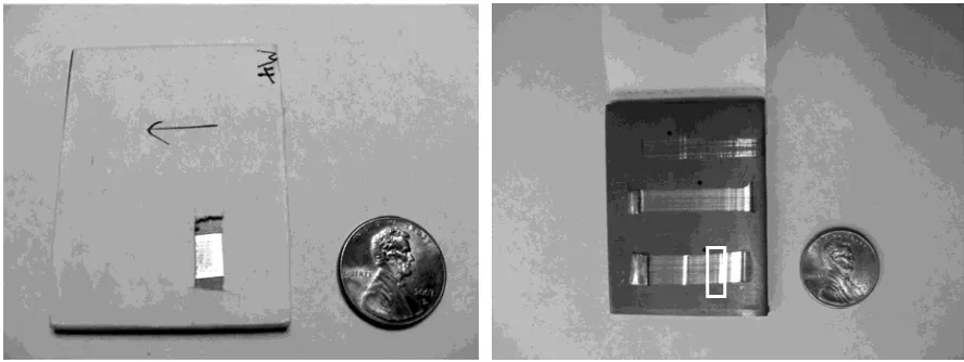
Figure 2. After making an initial assessment, the blinders were removed and the examiner was
given the opportunity to make a second assessment based on a view the entire sample. In each
case, examiners were asked to render an opinion as to whether they were viewing a positive
identification, a positive elimination, or inconclusive, for reasons that will become apparent.
[image:15.612.83.527.402.569.2]
Figure 2: Image of a tool marked plate with a) blinder in place and b) removed, showing the
Names of examiners were not recorded, although demographic data was collected concerning the
experience and training of the volunteers. Of the 50 volunteers all except five were court
qualified firearm and tool mark examiners. Of the remaining five, two were firearms (but not
tool mark) qualified, two were in training, and one was a foreign national where a court
qualification rating does not exist. Volunteers were required to do a minimum of two comparison
pairs, and could do as many as they wished. Several chose to do the maximum number of
comparisons possible. Numbers were assigned to identify each volunteer during data collection;
afterwards the ID numbers were randomly mixed to preserve anonymity.
Examiners were asked to use whatever methodology they employed in their respective labs. This
caused some confusion initially and placed constraints on the volunteers since some labs never
use the term “positive elimination”, while others are reluctant to use the term “positive
identification” unless the examiner personally either makes the marks or knows more
information about them than what could be supplied in this study. After understanding this the
examiners were told the direction of the tool when making the mark and that the tool marks were
all made at the same angle from similar, sequentially made, flat blade screwdriver tips. Also,
examiners were told that for the purposes of the study they could consider the terms of “positive
elimination” or “inconclusive” to be essentially interchangeable.
Results and Discussion
The data obtained from the profilometer was used to test a series of hypotheses that are held as
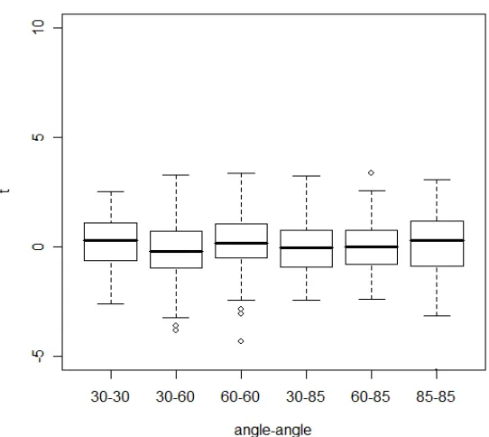
being true by tool mark examiners, Figure 3. The first and most fundamental assumption, that all
tool marks are unique, was tested by a comparison of marks made by different screwdriver tips at
the angles of 30, 60 and 85 degrees with respect to horizontal. The T1 statistic values are shown
in Figure 4 as a function of angular comparison. The data is plotted as box plots, the boxes
indicating where 50% of the data falls with the spread of the outlying 25% at each end of the
distribution shown as dashed lines. As stated previously, when using a T1 statistic a value
relatively close to 0 indicates that there is essentially no evidence in the data to support a
relationship between markings. For pairs of samples made with different screwdrivers (Figure 4)
the majority of the index T1 values produced by the algorithm fall near the 0 value; only 3
outlier comparisons had a T1 value greater than ± 4.
Figure 3: Summary of hypotheses tested in this study.
Hypothesis 1: The 50 sequentially produced screwdrivers examined in this study all produce uniquely identifiable tool marks
Hypothesis 2: In order to be identifiable, tool marks from an individual screwdriver must be compared at similar angles.
Figure 4: Box plots showing T1 results when comparing marks from different screwdrivers.
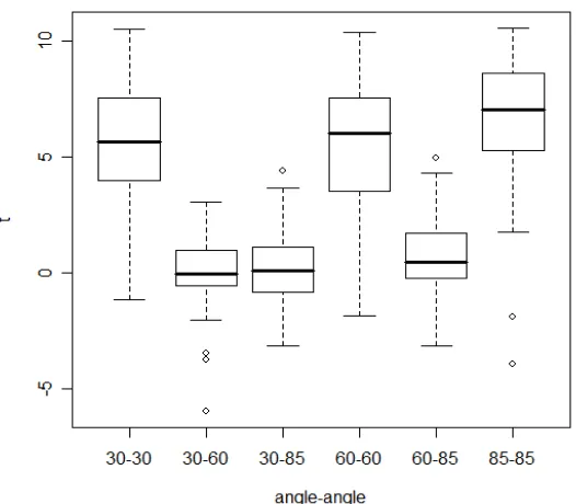
In comparison, Figure 5 displays indices computed using the algorithm from profilometer scans
of marks made by the same side of the same tool and compared as a function of angle. While
marks made at different angles still produce index values near 0, the T1 statistic jumps
dramatically when marks made at similar angles are considered. Clear separation is seen
between the 50% boxes, although overlap still exists when the outliers are considered.
Taken together, Figures 4 and 5 support Hypotheses 1 and 2. When comparing tool marks made
at similar angles with different tools, the resulting T1 values cluster near zero (Figure 4), but
when the same tool is used to make marks at similar angles, the T1 distributions are on
demonstrated by Figure 5 alone, since even among same-tool marks, only those made at the
same angle produce large T1 values.
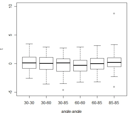
The last hypothesis considered was that when comparing tool marks made from screwdriver tips,
the marks must be made from the same side of the screwdriver; marks made using different sides
of the screwdriver appear as if they have come from two different screwdrivers. These results
are shown in Figure 6. The hypothesis is again supported because, as in Figure 4, the T1 values
cluster around 0 regardless of the angles used in making the marks, indicating no relationship
[image:19.612.176.439.374.604.2]between the samples.
Figure 5: Box plots showing T1 results when comparing marks obtained from the same side of
Figure 6: Box plots showing T1 results when comparing marks made from different sides of the
same screwdrivers.
The T1 values summarized in Figures 4 and 5 are individually replotted in Figure 7, with the
y-axis randomly varied (known as jittering) to create an artificial vertical separation that makes it
easier to view the data points. Known comparisons that should match and produce high T1
values are shown in black. Known “nonmatches” that should have T1 values near zero are
shown in gray.
Examination of these plots indicates that the algorithm operates best using data obtained at
higher angles than lower angles, i.e. the spread of black and gray spots is more defined for the 85
mark. As the angle of attack of the screwdriver with the plate increased the quality of the mark
increased. It was common to obtain marks that represented the entire screwdriver tip at high
angles, while marks at lower angles were often incomplete [5]. Algorithm performance also
appears more efficient at reducing false positives than it does in eliminating false negatives. At
all angles known matches were found with very low T1 values, while nonmatches with high T1
values were very limited.
While T1 is a much more stable index of match quality than R-value, problems still remain in
establishing an effective, objective standard for separating true matches from nonmatches.
Ideally, when employing standard U-statistic theory the critical T1 values separating the regions
of known matches (black data points) and known nonmatches (gray data points) should remain
constant for all data sets. Examination of Figure 7 shows that this is not the case. For example,
reasonable separation for the 30 and 60 degree data appears to be somewhere around a T1 value
less than 5, but rises to approximately 7 for the 85 degree data. This variation is most likely due
to lack of complete independence among the correlations computed in each sample, arising from
the finite length of each profilometer trace.
For the reasons discussed above, assigned threshold values indicating “Positive ID” and
“Positive Elimination,” and denoted by black lines on the graphs of Figure 7, were chosen based
on a K-fold cross validation using 95% one-sided Bayes credible intervals. Specifically, the
lower threshold is a lower 95% bound on the 5th percentile of T1 values associated with
percentile of T1 values associated with matching specimen pairs. The region between these two
threshold values is labeled “Inconclusive”. A Markov Chain-Monte Carlo simulation was used
to determine potential error rates.
Using this method the estimated error rates are as follow. For comparisons made at 30 degrees
the estimated probability of a false positive (i.e. a high T1 value for a known nonmatch
comparison) is 0.023. In other words there is a possibility of slightly over two false positives for
approximately every 100 comparisons. The estimated probability of a false negative is 0.089, or
almost 9 true matches having a low T1 value per every 100 comparisons. The cross-validation
method used ensures that all the data have similar error rates, and the rates found for the 60 and
85 degree data are approximately 0.01 and 0.09 for false positives and false negatives,
respectively. What is most noticeable is that the T1 lower threshold value for the 85 degree data
is much larger than for the 30 and 60 degree data, being 4.10 vs 1.34 and 1.51, respectively.
This suggests that a more distinct difference is required to classify nonmatches for the 30 and 60
degree cases than is true for the 85 degree case. This, in turn, results in a corresponding increase
for the estimated inconclusive error rates, which are 0.103, 0.298, and 0.295 for the 85, 60 and
30 degree data, respectively. It would, of course, be possible to shift these error rates, i.e.
produce fewer false negatives at the expense of more false positives, by altering the percentiles
-10 -5 0 5 10 15 30 Degrees T1 De n s it y Matches Nonmatches a.
-5 0 5 10 15
60 Degrees T1 D ensi ty Matches Nonmatches b.
-10 -5 0 5 10 15
Figure 7: Summation of the T1 values from comparisons made at a) 30 degrees; b) 60 degrees;
and c) 85 degrees.
Association of Firearm and Tool mark Examiners Study
Results of the computerized analysis of specimen pairs was compared to expert evaluations of
the same samples made by volunteer examiners at the 2008 Association of Firearm and Tool
mark Examiners seminar. However, before the algorithm performance can be discussed in
comparison to the data obtained at the Association of Firearm and Tool mark Examiners seminar
using human volunteers, a brief consideration of the constraints experienced by the examiners is
in order. Firstly, it should be recognized that the conditions under which the examiners rendered
an opinion would ordinarily be regarded as restrictive or even professionally unacceptable.
Without having the tool in hand, or without being permitted to make the actual mark for
comparison, tool mark examiners were forced to make assumptions they would not make in an
actual investigation. For example, without having the screwdriver tip in hand the examiners did
not know whether the mark they observed represented the entire width or only a portion of the
screwdriver blade. Secondly, given this uncertainty about how the specimen was made,
examiners tended to be more conservative in their willingness to declare a positive identification
or elimination. During the course of the Association of Firearm and Tool mark Examiners study
several examiners commented that typical lab protocol would require them to have physical
access to the subject tool before rendering a “positive identification” judgment. Finally,
analysis. Thus, while privately saying they felt a comparison was a “positive elimination” (given
their knowledge of the test being conducted), lab protocol required an opinion of “inconclusive”
to be rendered. Such policies are put in place since the signature of a tool may so change during
use that a mark made at one point in time may not resemble a mark made with the same tool at a
different point in time, e.g., after the tip has been broken and/or re-ground. In such cases
positive elimination is only allowed if the class characteristics of the marks are different.
When viewed in light of these constraints, some interesting observations concerning the
algorithm performance are apparent. In a small number of cases (12 out of 252 comparisons),
when examining the entire tool mark after first viewing only the restricted area where the
profilometer scans were obtained, examiners changed their opinion from inconclusive to either
positive ID or positive elimination. This indicates that algorithm performance might be
improved simply by increasing the amount of data processed. This may be achieved, for
example, by ensuring that the profilometer scans span the entire width of the mark or possibly by
considering a number of scans taken at locations dispersed along the entire length of the
available mark.
In a slightly smaller number of cases, comparisons between specimens made by the same
screwdriver that were not conclusively identified as such by the algorithm also presented
problems for the examiners. Five true matches that received low T1 values and were classified
as a positive elimination by the algorithm were examined during the Association of Firearm and
elimination” on one occasion, and one particular comparison sample (designated MW4) was
rated this way seven times. Thus, while examiners in general were vastly superior to the
algorithm in picking out the matches, both the algorithm and the examiners had more trouble
with some true matches than with others.
Close examination of the sample that was most often problematic for examiners (i.e. MW4) was
conducted and the images obtained are shown in Figure 8. Figure 8a shows the side-by-side
comparison of the marks, where no match is seen. Note that the mark width matches extremely
well, and the entire mark seems to be present. Figure 8b shows the samples positioned where the
true match is evident. It can be seen that each mark only represents a portion of the screwdriver
blade width, predominately from the two sides of the tip. A match is only possible if the marks
are offset, allowing the opposing “edge” sections (which actually were produced by the middle
of the screwdriver blade) to be viewed side-by-side.
Figure 8: Sample MW4. a) Tool marks placed so that assumed edges align. B) Correct placement
required for positive identification.
This sample points out weaknesses in the study conducted at Association of Firearm and Tool
mark Examiners as well as in the laboratory tests of the algorithm. In a screwdriver mark
comparison it is common for examiners to use the edges of the marks as initial registration points
for the start of an examination. Since examiners make the comparison marks themselves they
are well aware of the edge markings, if not for the evidence marks, at least for the marks they
produced. In the Association of Firearm and Tool mark Examiners study, such information was
not provided and may have led to some false assumptions. For example, in the majority of cases
the volunteers were under some pressure to quickly conduct a comparison before, e.g. the next
meeting session started, or so that another examiner could use the equipment, etc. Due to these
time constraints, samples often were placed on the stages of the comparison microscope for the
volunteer, giving the examiner little or no time to observe the macroscopic appearance of the
mark. Without the benefit of seeing the size of the entire mark, and given the identical widths of
the two partial marks for sample MW4 when initially viewed using the comparison microscope,
the assumption that the entire width of the screwdriver blade was represented would be a natural
one. However, such an assumption could easily lead to an inconclusive or positive elimination
conclusion, especially if the examiner was being conservative due to lack of information
The problem described above essentially relates to the examiners having a lack of a point of
reference or registry of the mark for the comparison. The same could be said of the algorithm
and the manner in which it performs, since no point of registry exists to indicate when the data
being acquired is actually coming from a tool-marked region or from the unmarked plate. All of
the profilometer scans analyzed by the algorithm were run using the same set of sampling
parameters. However, the initial positioning of the stylus was inexact. For incomplete marks,
large regions of the unaffected lead plate were also scanned in order to keep the file sizes
consistent and this lack of registry could have affected algorithm performance. This is not
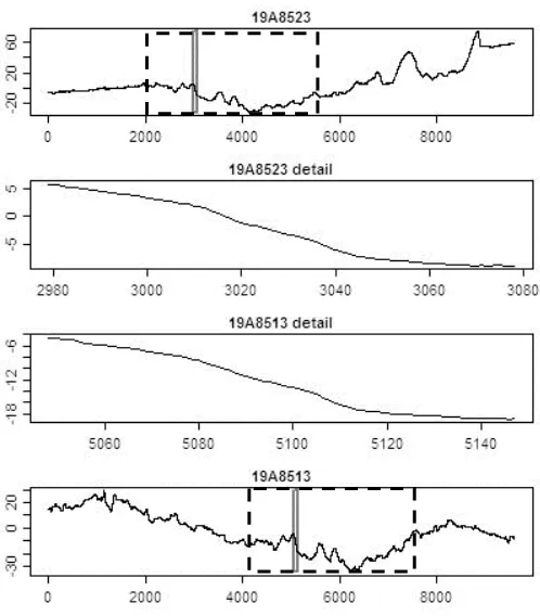
immediately evident if one examines the raw profilometer traces, Figure 9. In this figure the top
and bottom traces show the entire scans while the two middle traces show the matched details
found within the two corresponding solid rectangles superimposed on the top and bottom traces.
At first sight the two scans do appear quite different, as the offset in the scans, revealed during
examination at Association of Firearm and Tool mark Examiners, is not immediately evident in
the data files.Given observation of Figure 8, one can mark the approximate location of the
region that is common between the two traces; this is shown in Figure 9 by the dashed
rectangles. In this case, paired validation windows, displaced equal amounts in either direction
may return a low T1 value since the majority of either scan is not held in common with the other.
In other words, there is a high probability that the validation windows fall in regions where no
correspondence between plates exists (see Figure 8b). Thus, what should be a match is rated as a
Figure 9: Profilometer data showing results from comparison MW4. The match region is shown
by the solid rectangle. Dashed rectangles show the approximate location of the common region
revealed in Figure 8.
A somewhat different problem is revealed when traces from true nonmatch samples are
examined, Figure 10. In these instances, the optimization step may identify windows at extreme
edges of the two traces as being most similar. Given the nearness of the match to the ends of the
traces, the random selection of paired, rigid-shift windows during the validation step is severely
constrained. For the example shown in Figure 10a the match region (denoted by solid
taken for each pair of verification windows must always fall to the left of the match region.
While this may be less than desirable, the entire mark is still available for validation and a large
number of rigid-shift windows spaced across the entire length of the file should be sufficient to
produce good separation between this accidental match and the T1 values of a true match.
However, this is not true for the true non-match shown in Figure 10b. In this case the windows
identified in the optimization step as being most similar are at opposite ends of the compared
data traces. The distances of possible rigid translations are constrained to a short distance to the
left of the top profile and a short distance to the right of the bottom profile. Thus, the majority of
the mark cannot be used in the validation step for this accidental match. If the regions in the
immediate vicinity of the accidental match are also similar, high T1 values may be returned due
to the constrained sampling parameters, giving results that cannot be separated from a true
a. b.
Figure 10: Comparisons of traces obtained from four different screwdrivers that were rated as
possible matches by the algorithm. Match areas denoted by thin rectangles. Good agreement
found at a) similar and b) opposite ends of the traces resulted in high T1 numbers for known
non-matching pairs.
The above discussion suggests that further development of the algorithm to incorporate
additional data concerning the region of the profilometer trace that is actually tool-marked and/or
the location of the tool edge might improve its performance. While tool mark examiners do not
directly use features such as these as a basis for identification, they do use it indirectly in
establishing a context for the comparison. Such information, routinely and quickly noted by a
human examiner, is unavailable to the current algorithm. The algorithm treats all possible pairs
of trace windows the same way and functions under the assumption that all marks analyzed are
essentially the same, i.e., it assumes the screwdriver tip has completely marked the lead plate and
that no unmarked regions exist. This clearly is not the case. At this time it appears the best way
to enhance algorithm performance is to ensure that all comparison windows (i.e. Match and
Validation) are taken from regions representing the true marked surface of the lead, and that
most-similar windows found at the trace edges are used as a basis for match identification only if
As a final comment, it should be noted that all types of volunteers (practicing examiners,
trainees, retired examiners) were involved in the study, with records kept as to the experience of
the participant. Examination of the demographic data in relation to the results showed no
significant difference between experienced examiners and rather newly qualified examiners or
those in training; all performed equally well.
Summary and Conclusions
The analysis described here for comparing two tool-marked plates is a substantial improvement
over simply identifying regions of highest correlation. It does this by producing a
non-parametric Mann-Whitney statistic, here called T1, obtained through an optimization step
followed by a validation step as a measure of evidence for tool mark matching. When used in
evaluating the three hypotheses tested, namely, the uniqueness of tool marks, the necessity of
comparing marks at similar angles, and the uniqueness of different sides of screwdriver blades,
the T1 statistic results constitute support for the experiential knowledge of tool mark examiners.
Analysis of algorithm performance in light of actual examiner results reveals deficiencies in
algorithm performance that can now be addressed. Increasing the data input, possibly by
including more scans spread over a larger tool mark area and incorporating contextual
information normally available to examiners, such as the presence of partial scans and reference
example, prohibit the identification of opposite-end windows in the optimization step as potential
match segments.
It is clear that examiner performance was much better than the algorithm. While the 20 samples
examined at Association of Firearm and Tool mark Examiners represent only a subset of the total
comparisons examined using the algorithm, they did contain those samples that were most
definitively misclassified by the algorithm. For example, of the 20 true-match pairs shown to the
Association of Firearm and Tool mark Examiners volunteers, the algorithm correctly identified
10 of the 20 samples unambiguously; the remaining 10 were listed either as inconclusive or
misidentified as a false negative. In comparison, only 11 out of 126 volunteer examinations
resulted in false negative classification of true match pairs, primarily from sample MW4 (7 out
of 11). Further, the Association of Firearm and Tool mark Examiners volunteers reported no
false positives at all. (N.B. The caveat must be added that the terminology used in the previous
statements regarding errors is not entirely consistent with examiner protocols and should not be
construed by the reader to suggest that the examiners erred. Examiners are trained to render an
opinion of positive identification only when no doubt exists in their minds. Thus, a false
negative only suggests that the examiner was not fully persuaded.)
The authors are extremely grateful to Wayne Buttermore of Leica Microsystems and Kevin
Boulay and Mike Howell from Leeds Precison Instruments for providing comparison
microscopes. Without their assistance much of this study could not have been conducted. We
are also grateful to officers and organizers of the 2008 Association of Firearms and Tool mark
Examiners Training Seminar held in Honolulu, especially Jim Hamby, Cindy Saito and Curtis
Kubo, for helping us with the booth and getting volunteers for the study. Finally, we gratefully
acknowledge the assistance of all the AFTE members who took the time to participate in our
study. This work was supported by the National Institute of Justice under contract
2004-U-R-088, and was performed in part at Ames Laboratory, which is operated under contract No.
W-7405-Eng-82 by Iowa State University with the US Department of Energy.
References
1. Bisotti A. A Statistical Study of the Individual Characteristics of Fired Bullets. Journal of
Forensic Science 1959 Jan:4;1:34-50.
2. Bonfanti MS, DeKinder J. The Influence of the Use of Firearms on their Characteristic
Marks. Association of Firearm and Tool mark Examiners 1999;31:3:318-323.
3. Bonafanti MS, De Kinder J. The Influence of Manufacturing Processes on the Identification
of Bullets and cartridge cases – A Review of the Literature. Science and Justice 1999; 39:3-10.
4. Bisotti A, Murdock J. Criteria for Identification or State of the Art of Firearm and Tool mark
Identification. Association of Firearm and Tool mark Examiners 1984 Oct:16;4:16-24
5. Report by a committee for the National Research Council for the National Academy of
6. Faden D, Kidd J, Craft J, Chumbley LS, Morris M, Genalo L,. Kreiser J, Davis S.
Statistical Confirmation of Empirical Observations Concerning Tool mark Striae. Association of
Firearm and Tool mark Examiners Journal 2007 Summer;39;3:205-214.
7. Baldwin D, Morris M, Bajic S, Zhou Z, Kreiser MJ. Statistical Tools for Forensic Analysis