International Journal of Innovative Technology and Exploring Engineering (IJITEE) ISSN: 2278-3075,Volume-8, Issue-10S, August 2019
Abstract: In this research, an automated and customized neoplasm segmentation methodology is given and valid against ground truth applying simulated T1-weighted resonance pictures in twenty five subjects. a replacement intensity-based segmentation technique known as bar graph primarily based gravitational optimization algorithm is developed to segment the brain image into discriminative sections (segments) with high accuracy. whereas the mathematical foundation of this rule is given in details, the appliance of the projected rule within the segmentation of single T1-weighted pictures (T1-w) modality of healthy and lesion MR images is additionally given. The results show that the neoplasm lesion is divided from the detected lesion slice with eighty nine.6% accuracy..
Keywords : neoplasm segmentation methodolo, T1-weighted resonance .
I. INTRODUCTION
Detection and segmentation of tumor greatly impacts the treatment and watching of the patient throughout the medical care [1]. Additionally, it is advantageous for general modeling of pathological brains and also the construction of pathological brain atlases [2]. Tumor detection and segmentation is done either manually or mechanically. Manual segmentation is usually valuable, time intense, tedious, and suffers from lack of permanent convenience, irresponsibleness and dependability [1, 4]. Therefore, an efficient automatic tumor segmentation rule is clinically helpful.
Among completely different medical imaging techniques, resonance imaging (MRI) is most generally used because of its noninvasive procedure, which in contrast to alternative medical imaging techniques permits the differentiation of soppy tissues with high resolution. Another advantage of imaging is that it produces multiple pictures of identical tissue with distinction mechanisms whereas applying different image acquisition protocols and parameters [3]. These multiple imaging modalities give completely different reasonably anatomical data for identical tissue. Since lesions have similar intensities to the traditional tissues, multi-spectral adult male pictures are used for lesion segmentation. However, multispectral adult male pictures don't seem to be forever simple to use because of completely
Revised Manuscript Received on July 08, 2019.
P. Ratha*, Assistant Professor, Department of computer science,
Bharathidasan university model college, Aranthangi. Email:-
Dr. B. Mukunthan, Associate professor, Dept of computer science, Sri Ramakrishna College of Arts & Science, Coimbatore. Email :-
different reasons [4]. Firstly, acquiring such data is not always feasible due to patient disease severity and time restriction. Secondly, collecting anatomical multi-spectral MR images is expensive. Thirdly, multimodal MR images data are not consistent and aligned, thus some prior interference of the researcher in the process for atlas registration is required [5]. Based on these limitations, detecting and segmenting the tumor lesion based on single anatomical MR modality is necessary and important. There square measure many alternative approaches for automatic growth detection and segmentation [6-12], which might be classified into region-based and contour-based ways [9]. though there square measure many segmentation ways like thresholding [15], region growing [16], and cluster [10, 17], they're not simply applicable on the brain lesion identification domain as a result of the intensity similarities between brain lesions and a few traditional tissues.
Most of the segmentation ways mentioned and reportable in growth segmentation field suffers from dependency on multi-parameter MRI information [6], multi-scale classification [11], and non-noisy and high-resolution information [13]. Moreover, sometimes the dependency on native or world registration of brain pictures to AN anatomical atlas could be a disadvantage of majority of studies [7, 10]. in addition, besides having high procedure quality, not being totally machine-driven is that the different limitation [12, 14]. to handle the above-named shortcomings, we tend to propose a histogram-based attraction improvement rule (HGOA), that is predicated on applying increased attraction improvement rule on brain bar graph.
The contributions of our projected rule square measure in its freedom from previous atlas registration further as multi-spectral MRI, and practitioner low-level formatting. the opposite contributions will be listed as this methodology is totally automatic and computationally economical since it applies constant rule for lesion detection and segmentation. we've got conjointly increased the first attraction improvement rule to increase it for n-dimension and conjointly small the chance of being treed into a neighborhood best answer.
Brain Tumor Detection and Segmentation
using Histogram and Optimization Algorithm
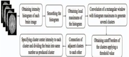
Fig. 1: Flowchart of the seven steps histogram-based brain segmentation algorithm
The proposed algorithm begins with three main stages to provide several brain segments of the original image. These stages are: firstly, application of a weighted average technique on the brain histogram; secondly, convolution of a rectangular window with the histogram maximum bars; and thirdly, connection of the cutoff borders after thresholding. Once these are done, application of an enhanced optimization algorithm-n-dimensional gravitational optimization algorithm (NGOA)- results in the desired number of brain segments. Intensity widths of the generated segments on the brain histogram are used for lesion detection and segmentation. Three criteria – sensitivity, specificity, and accuracy – are applied to evaluate the algorithm performance.
The n-dimensional gravitational optimization algorithm is based on the principle of gravitational fields. It is motivated by the idea of gravitational forces between several masses and Newtonian laws of motion [18]. The objective function is a non-linear function of variables, which are called masses and defined based on brain image histogram analysis. The value of the objective function determines the movements and new locations of the masses. The masses are the length of the averaging window, the length of a rectangular convolution window, and the threshold of cutoff borders. The algorithm is iterated until a predefined iteration number or convergence is met.
This research is organized as follows. In Section II, the histogram-based gravitational optimization algorithm is explained followed by section III which is about data acquisition and preprocessing. Results are discussed in section IV and section V concludes the paper.
II. HISTOGRAM-BASEDGRAVITATIONAL
OPTIMIZATIONALGORITHM
In this section histogram-based gravitative improvement algorithmic rule (HGOA) is explained in details. This algorithmic rule is separated into 2 elements as “histogram-based brain segmentation algorithm” and “gravitational improvement algorithm”.
Histogram-based brain segmentation algorithmic program starts by building the image intensity bar chart. it's assumed that the native maximums of the bar chart are probably representative of varied segments within the brain. Therefore, the amount and also the worth of the bar chart native maximums is associated with the amount and also the center worth of segments, severally. albeit in magnetic resonance imaging every constituent is truly a voxel, we are going to treat every constituent as happiness to 1 section.
Therefore, the space from one native most to a different one is split proportionately between the 2 native most bars to hide the full intensity vary. With dividing proportionately, the native most worth affects the breadth of every section. Doing so, the brain is mesmeric to constant variety of its histogram’s native maximums. However, if the required variety of brain segments is totally different from the overall variety of brain histogram’s native maximums, a changed improvement algorithmic program known as n-dimensional attractive force improvement algorithmic program helps to dynamically section the brain into the required variety of segments. For this purpose, it's necessary to outline associate improvement method within which the target operate is made from the brain bar chart analysis. associate improvement method is outlined to attenuate the distinction between the achieved variety of segments and also the desired variety of segments. The improvement method works primarily based upon associate reiterative calculation of associate objective operate, that is made from histogram-based brain segmentation algorithmic program.
A) Histogram-based Brain Segmentation Algorithm The histogram-based brain segmentation algorithm is summarized in Fig. 1 highlighting the underlying seven-steps of the proposed algorithm. The details of these steps can be found in our previous work [19].
Step1: Calculate the image intensity histogram
Step2: Apply a weighted averaging technique on the image histogram
Step3: Extract the local maximum from the averaged image histogram
Step4: Convolve a rectangular window with the intensity histogram peaks obtained from step 3
Step5: Obtain the lower and the upper cutoff borders for all segments using a threshold value
Step 6: Connect the upper cutoff border of nth segment to the lower cutoff border of (n+1)th segment proportionally to the distribution value of the calculated intensity histogram from step 4
Step 7: Allocate a specific intensity value to each generated segment.
The brain is segmented according to the number of clusters, the intensity of the cluster center, and the cutoff borders of generated clusters. In order to automate this process, an optimization process is applied to minimize the difference between the number of generated brain segments and the desired number of brain segments. There are three variables that influence this difference. These variables are the length of averaging window described in step two, the length of convolution window described in step four, and the threshold value described in step five. The N-dimensional gravitational optimization algorithm is explained in the next part.
B) N-Dimensional Gravitational Optimization Algorithm
The second part of our proposed algorithm is an enhanced optimization algorithm called n-dimensional gravitational optimization algorithm. In order to achieve the desired number of the brain segments,
[image:2.595.56.266.51.143.2]International Journal of Innovative Technology and Exploring Engineering (IJITEE) ISSN: 2278-3075,Volume-8, Issue-10S, August 2019
histogram-based brain segmentation algorithm. The objective function is defined as the squared difference between the desired number of segments and the achieved number of segments. As it was explained before, if we need to segment the brain to four segments, the desired number of brain segments would be four.
NGOA utilizes the principles of gravitational field. Similar to space gravitational algorithm [15], this algorithm is motivated by a simulation of several space masses to search for the heaviest mass. As our contribution, we expand the search over the n-dimensional search space while in [15] masses are modeled in 2D. Some formula modifications are also considered, which decrease the possibility of masses being drawn into a local optimal solution.
Random selection of K sets of n-dimensional masses and the iteration number launch the GOA. In other words, for the n-dimensional search space, the position of the Ith mass can be represented by an n-dimensional vector the velocity by and acceleration vector by . Therefore the total size of population is a (K x N) matrix. In NGOA, the gravitational force on the object is calculated as:
where mi is defined as inverse of objective function value in a minimization problem, equation (2).
In a maximization objective function, there is no need to inverse the objective function value. In equation (2), is added to denominator to prevent dividing one by zero when the distance between masses becomes zero. The calculation of the gravitational force on the Ith mass, by assuming a unit time length, the new speed of the Ith mass is calculated as equation (3):
The function represent the acceleration of mass Xi , and the function min finds the minimum acceleration between all masses. Here, g is the gravity constant. Having the speed of the system at time (t + 1) and the previous location of the Ith mass at Xi (t), the position in the next iteration is adjusted by:
It is recommended to add a random movement of the particles up to a specific iteration number in order to add a random factor in optimization to increase the convergence rate. This happens by adding a random vector to some of the worst variables. The random variable should not take the selected variables outside of the boundaries. In addition, replacing the worst variables of each iteration with the best of past generations moves the average of all point toward the optimal points.
Here, N is three regarding to the three variables, which affect on the objective function. These three variables are “G” i.e. the length of the averaging window, “W ” i.e. the length of a rectangular convolution window (Win), and Thr i.e. the threshold of cutoff borders as explained in section II.A. The equations (1) to (4) are iteratively calculated until the objective function or the iteration number is met.
III. DATAACQUISITIONANDPREPROCESSING
A.Data Acquisition
For experiments, 25 simulated data of brain T1 weighted-MRI images were acquired from neuroimaging tools and resources (NITRC) [1], [20]. The data was generated using cross-platform simulation software called TumorSim.
The experiment has been developed using MATLAB R2012a and is applied on T1-weighted MRI images of 25 subjects. Each subject has 181 T1-weighted slices. The ground truth is presented in the database for final evaluation.
B.Preprocessing
Preprocessing includes three parts as background segmentation, noise reduction using low pass filter, and normalization. Due to the prior knowledge of the background intensity values, it is necessary to exclude the back ground from the calculations wherever the histogram of the image is evaluated.
Gaussian Filter is a low-pass spatial frequency filter where all elements in this filter are weighted according to a Gaussian distribution. Depending on the mean and the
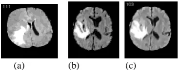
variance value, (µ, ), in the Gaussian distribution, the convolution of this kernel with the image results in a smooth image [22]. Result of applying Gaussian filters with two
different sigma is represented in Fig. 2(b) and 2(c). It is seen that the result of Gaussian filter, depends on the value of
sigma . Here, the low value for is preferred. By dividing the intensity values by the maximum intensity, normalized image is prepared.
I. RESULTS
A.MRI Brain Segmentation
Original T1-weighted image of patient 1 with the tumor lesion which we call it P1 is presented in Fig. 2(a). The segmentation of P1 into two, three and four segments is depicted in Fig. 3. Correspondingly, Fig. 4 displays the segmentation of P1 into five, six and twelve segments. It can be seen that after 4 levels of segmentation the tumor lesion appears in the segmented image. It can also be seen that in high levels of segmentation, some of the segments are visually indiscriminative; however, there is still a clear appearance of the tumor in the segmented image.
(a) (b) (c)
Fig. 2: Original P1 with tumor lesion (a), the filtered image using Gaussian filter with , (b), and with
(c)
(a) (b) (c)
Fig. 3: Segmentation of P1 into two (a), three (b), and four (c) segments
(a) (b) (c)
Fig.4: Segmentation of P1 into five (a), six (b), and twelve (c) segments
Fig. 5 shows the original T1-weighted image of P2, which does not have tumor lesion. It also indicates segmentation of P2 into four and five segments. Fig. 6 illustrates the original T1-weighted image P3 with the tumor lesion, and its segmentation into four and five segments. Fig. 9 and 10 show the result of histogram-based brain segmentation algorithm’s steps for P1, which includes lesion for four and five level of segmentation, respectively. Fig. 9(a) and 10(a) correspond to image histogram after step 2. Fig. 9(b) and 10(b) show the local maximums of the histogram in step 3. Fig. 9(c) and 10(c) illustrate results of step 4. Fig. 9(d) and 10(d) show the results of step 5 and 6. In all, red dots are initial lower and upper cutoff borders, which are result of step 5, and black dots are final lower and upper cutoff borders, which are result of step 6 of histogram-based brain segmentation algorithm.
(a) (b) (c)
Fig. 5: Original P2 healthy (a), segmentation of P2 into four (b), and five segments (c)
[image:4.595.56.242.163.239.2]
(a) (b) (c)
Fig. 6: Original P3 with tumor lesion (a), segmentation of P2 into four (b), and five segments (c)
Fig. 11 and 12 show the result of histogram-based brain segmentation algorithm’s steps for P2, which is healthy for four and five level of segmentation, respectively. Fig. 11(a) and 12(a) correspond to image histogram after step 2. Fig. 11(b) and 12(b) show the local maximums of the histogram in step 3. Fig. 11(c) and 12(c) illustrate results of step 4. Fig. 11(d) and 12(d) show the results of step 5 and 6. As mentioned before, red dots are initial lower and upper cutoff
lower and upper cutoff borders, which are result of step 6 of histogram-based brain segmentation algorithm.
Tumor Lesion Detection
With comparison of position of cutoff borders, it is clear when brain is segmented into four segments, the cutoff borders position of second segment differs for healthy and lesion slices. The following criterion is defined as the condition for lesion slice detection as:
where X low [2] refers to lower cutoff boundary of second segment, and X up [2] refers to upper cutoff boundary of second segment. q1 is specified as 2.25, and q2 is specified as 4.85. Tumor slices are detected with 89.3% accuracy.
B.Tumor Lesion Segmentation
After detection of slices together with neoplasm lesion, the image is segmented into four and 5 segments. The neoplasm is found within the second phase. so with extracting the second phase, the neoplasm lesion are often segmented. results of this step is delineate in Fig. 7 and 8. it's discovered that combination of mesmeric neoplasm’s when segmenting the brain into four and 5 segments will cowl the tagged tumor higher. Therefore, when segmenting the brain into four and 5 segments, the second segments square measure accumulated exploitation logical OR. In line with established apply, [5], [21], [22], sensitivity, specificity, and accuracy square measure used, for analysis of the algorithmic rule performance:
where true positives (TP) are voxels correctly identified as lesion, true negatives (TN) are voxels correctly identified as healthy, false positives (FP) are voxels incorrectly identified as lesion, and false negatives (FN) are voxels incorrectly identified as healthy. In order to evaluate the algorithm performance, the segmented lesions are compared with the ground truth. Result of lesion segmentation for 25 subjects using histogram-based gravitational optimization algorithm for four segments and five segments and their combination is presented in Table 1.
(a) (b) (c) (d)
Fig. 7: Original P1 with tumor lesion (a), segmented tumor after four levels of segmentation (b), after five levels of segmentation (c), accumulation of segmented tumor of four and five levels (d)
[image:4.595.47.288.467.640.2] [image:4.595.305.549.577.645.2] [image:4.595.305.561.694.839.2]
International Journal of Innovative Technology and Exploring Engineering (IJITEE) ISSN: 2278-3075,Volume-8, Issue-10S, August 2019
lesion (a), segmented tumor after four levels of segmentation (b), after five levels of segmentation (c), accumulation of segmented tumor of four and five levels (d)
[image:5.595.58.289.95.225.2]
Fig. 9: 4 level of segmentation of P1 (with tumor lesion): The intensity histogram after step 2 (a), result of step 3 (b), results of step 4 (c), and the results of step 5 and 6 (d)
Table 1: Result of lesion detection using histogram-based brain segmentation algorithm for four segments and five segments and their combination
IV. CONCLUSION
A new brain segmentation algorithmic rule known as bar graph primarily based attractive force optimization algorithm was proposed. the automated brain segmentation into distinct segments was conferred. The tumor detection and segmentation victimization single modality T1-weighted MR images with comparable and promising accuracy was enforced. Simplicity, low procedure complexness, independence of multi-spectral adult male pictures, multi-scale classification, and anatomical atlas registration area unit distinguished blessings of this work. Moreover, same algorithmic rule is employed for tumor detection and segmentation.
The disadvantage of the conferred approach is that the rate of false positives. In future, we have a tendency to will devise a technique to cut back the false positive within the planned system. Furthermore, it's supposed to evaluate the algorithm on other MRI modalities. Finally, additional focuses on amending the present technique to achieve a system in additional clinically general applications are going to be done. The potential outcome is outstanding for medical field and justifies any studies.
REFERENCES
1. M. Prastawa, E. Bullitt, G. Gerig, “Simulation of brain tumors in MR images for evaluation of segmentation efficacy”, Medical Image Analysis, 13: 297–311, 2009.
2. A. Toga, P. Thompson, M. Mega, K. Narr, R. Blanton, “Probabilistic approaches for atlasing normal and disease-specific brain variability”, Anatomy and Embryology 204 (4): 267–282, 2001.
3. D. Mortazavi, A. Z. Kouzani, H. Soltanian-Zadeh, “Segmentation of multiple sclerosis lesions in MR images: a review”, Neuroradiology, 2011.
4. Y.Kabir, M.Dojat, B.Scherrer, F.Forbes, C.Garbay, “Multimodal MRI segmentation of ischemic stroke lesions”, Proceedings of The 29th annual international conference of the IEEE EMBS, 2007.
5. S. Shen, A. Szameitat, A. Sterr, “Detection of infarct lesions from single MRI modality using inconsistency between voxel intensity and spatial location a 3-D automatic approach,” IEEE Trans 2008
6. M.C. Clark, et al. “Automatic tumor-segmentation using knowledge-based techniques”, IEEE Trans. Med. Imaging, 187– 201, 1998.
7. M. Kaus, et al. “Automated segmentation of MR images of brain tumors”. Radiology, 218 (2), 586–591, 2001.
8. M. Prastawa, et al. “A brain tumor segmentation framework based on outlier detection”. Med. Image Anal. 8, 275–283, 2004.
9. H. Khotanlou, et al. “3D brain tumor segmentation in MRI using fuzzy classification, symmetry analysis and spatially constrained deformable models”, Fuzzy Sets and Systems, 160: 1457-1473, 2009.
10. K. Van Leemput, et al. “Automated Model-Based Tissue Classification of MR Images of The Brain”, IEEE Trans. Med. Imag., 18, 897–908, 1999.
11. J.J. Corso, E. Sharon, A. Yuille, “Multilevel segmentation and integrated Bayesian model classification with an application to brain tumor segmentation”, MICCAI2006, Copenhagen, Denmark, Lecture Notes in Computer Science, 4191, 790–798, 2006.
12. G. Moonis, J. Liu, J.K. Udupa, D.B. Hackney, “Estimation of tumor volume with fuzzy-connectedness segmentation of MR images”, American Journal of Neuroradiology, 23: 352–363, 2002.
13. W. Dou, et al., “A framework of fuzzy information fusion for segmentation of brain tumor tissues on MR images”, Image and Vision Computing, 25:164–171, 2002.
14. A. Lefohn, J. Cates, R. Whitaker, “Interactive, GPU-based level sets for 3D brain tumor segmentation”, Technical Report, University of Utah, April 2003.
15. G. Lemieux et al., “Fast, Accurate, and Reproducible Automatic Segmentation of the Brain in Weighted Volume MRI Data”, Magn. Reson. Med., 42, 127–135, 2002.
16. H. Tang et al., “MRI Brain Image Segmentation by MultiResolution Edge Detection and Region Selection”, Comput. Med. Imag. Graph., 24, 349–357, 2002.
17. A.W.C. Liew & H. Yan, “An Adaptive Spatial Fuzzy Clustering Algorithm for 3-D MR image Segmentation”, IEEE Trans.Med. Imag., 22 (9), 1063–1075, 2003.
18. H. Ying-Tung, et al., “A novel optimization algorithm: space gravitational optimization," IEEE International Conference on Systems, Man and Cybernetics, 2005
19. N. Nabizadeh, et al, “Automatic Ischemic Stroke Lesion Segmentation Using Single MR Modality and Gravitational Histogram Optimization Based Brain Segmentation”, The 17th International Conference on Image Processing, Computer Vision, & Pattern Recognition, p207-213, 2013
20. Http://Www.Nitrc.Org/Projects/Tumorsim
21. A.P. Zijdenbos, et al. “Morphometric analysis of white matter lesions in MR images: method and validation”. Medical Imaging, IEEE Transactions on, 13(4): 716-724, 1994.
22. P. Anbeek, et al, “Probabilistic segmentation of white matter lesions in MR imaging”, Neuro Image, 21: 1037-1044, 2004
AUTHORSPROFILE
P. Ratha Assistant Professor, Department of computer science,
Bharathidasan university model college, Aranthangi. Email:-
.
Dr. B. Mukunthan Associate professor, Dept of computer science, Sri
Ramakrishna College of Arts & Science, Coimbatore. Email :-