Sliding Mode Control of MIMO Non-Square Systems via Squaring Matrix Transforms

Rochester Institute of Technology

RIT Scholar Works

Theses Thesis/Dissertation Collections

12-2013

Sliding Mode Control of MIMO Non-Square

Systems via Squaring Matrix Transforms

Tim Marvin

Follow this and additional works at:http://scholarworks.rit.edu/theses

This Thesis is brought to you for free and open access by the Thesis/Dissertation Collections at RIT Scholar Works. It has been accepted for inclusion in Theses by an authorized administrator of RIT Scholar Works. For more information, please [email protected].

Recommended Citation

Sliding Mode Control of MIMO

Non-Square Systems via Squaring Matrix

Transforms

By

Tim Marvin

A Thesis Submitted in Partial Fulfillment of the Requirements for Masters of Science in Mechanical Engineering

Approved by:

Dr. Agamemnon Crassidis – Thesis Advisor ____________________________________ Department of Mechanical Engineering

Dr. Jason Kolodziej ____________________________________ Department of Mechanical Engineering

Dr. Wayne Walter ____________________________________ Department of Mechanical Engineering

Dr. Alan Nye ____________________________________ Department of Mechanical Engineering

Department of Mechanical Engineering Rochester Institute of Technology

PERMISSION TO REPRODUCE THE THESIS

Sliding Mode Control of MIMO

Non-Square Systems via Squaring Matrix

Transforms

I, Tim Marvin, hereby grant permission to the Wallace Memorial Library of Rochester Institute of Technology to reproduce my thesis in the whole or part. Any reproduction will not be for commercial use or profit.

Date:_________________________ Signature:_____________________________

Abstract

In this thesis, a novel method for control of over- or under-actuated dynamic systems is

developed. The primary control method considered here is Sliding Mode Control which requires an inversion of the control input influence matrix. However, on many systems this matrix is non-square, requiring alternate methods in order to obtain the control solution. Some existing

solutions for this class of problems include pseudo-inversion such as the Moore-Penrose (which does not allow the design engineer to select the desired state to be controlled), dynamic extension (which is difficult to implement on large systems), and pseudo-inverse squaring transform

methods. While the squaring transform method solves the key issue in the Moore-Penrose method of not being able to select the desired control state, it still has been limited to systems with only one input. The current effort seeks to extend this squaring transformation method to multiple input systems and demonstrate the control allocation properties of the technique. By extending this method to multiple-input systems the technique becomes applicable to a wider range of real world problems, allowing designers to select and optimally control any desired state on multi-input-multi-output systems. This thesis examines the existing solutions for squaring of input influence matrices such as Moore-Penrose and dynamic extension, the transform method developed in previous work, and derives a multi-input extension to that method and also considers control allocation in the solution process. Simulations are then developed on a two-input, four mass-spring-damper system, and a multi-input longitudinal aircraft model to demonstrate the technique and characterize its performance in both sterile and noisy

Contents

Abstract ... 3

List of Figures ... 6

List of Tables ... 8

Nomenclature ... 9

Introduction ... 10

1 1.1 Background ... 10

1.1.1 Classical Control Theory and Methods ... 10

1.1.2 Modern Control Theory and Methods ... 10

Background work ... 16

2 2.1 Non-Square Systems ... 16

2.1.1 Moore-Penrose Pseudo-inverse ... 16

2.1.2 Dynamic Extension ... 16

2.1.3 Current Effort – Squaring Transformation Matrix ... 17

Theoretical Development ... 18

3 3.1 Squaring Transformation Matrix for Under Actuated Systems ... 18

3.2 MIMO Derivation ... 21

Results ... 24

4 4.1 Under-Actuated System Example ... 24

4.1.1 System Assumptions ... 24

4.1.2 State Space Model Derivation ... 25

4.1.3 Pseudo-Inverse Controller ... 29

4.1.4 Transformed Matrix Controller ... 30

4.1.5 Results and Comparison of Techniques ... 32

4.1.6 Control Allocation ... 36

4.2 Longitudinal Aircraft Model ... 40

4.2.1 Pseudo-Inverse Controller ... 41

4.2.2 Transformed Matrix Controller ... 42

4.2.3 Results and Comparison of Techniques ... 43

Conclusions ... 58

5.2 Future Work ... 58

Societal Impact ... 59 6

List of Figures

Figure 1: Example Mass-Spring-Damper System (image courtesy Aaron Yoon) ... 11

Figure 2: Four Mass-Spring-Damper System (image courtesy Markus Kottmann) ... 24

Figure 3: Free-body diagrams for four mass-spring-damper system ... 26

Figure 4: Four Mass Spring Damper Simulink Pseudo-Inverse Controller Model ... 30

Figure 5: Four Mass Spring Damper Transformed Matrix Simulink Model ... 32

Figure 6: Transformed Matrix Tracking Results ... 33

Figure 7: Pseudo-Inverse Tracking Results ... 33

Figure 8: Tracking Error ... 34

Figure 9: Comparison of Control Effort ... 35

Figure 10: Four Mass Spring Damper – Transformed Matrix - Control Allocation ... 37

Figure 11: Four Mass Spring Damper - Pseudo-Inverse - Control Allocation ... 37

Figure 12: Tracking Error - Control Allocation ... 38

Figure 13: Control Effort - Control Allocation ... 38

Figure 14: Non-Optimal Input - Tracking Results ... 39

Figure 15: Non-Optimal Input - Tracking Error ... 39

Figure 16: Non-Optimal Input - Control Effort ... 40

Figure 17: Longitudinal Terms of a Climbing Aircraft (image courtesy of NASA OLD) ... 41

Figure 18: Longitudinal Terms of a Descending Aircraft (image courtesy of NASA OLD) ... 41

Figure 19: Legacy Implementation ... 42

Figure 20: Moore-Penrose Pseudo-Inverse Controller ... 42

Figure 21: Transformed Matrix Simulink Implementation ... 43

Figure 22: Transformed Matrix Implementation Detail ... 43

Figure 23: Longitudinal Aircraft Model – Flight Path Tracking ... 44

Figure 24: Longitudinal Aircraft Model – Flight Path Tracking – Tracking Error ... 45

Figure 25: Longitudinal Aircraft Model – Control Effort – Flight Path Tracking ... 45

Figure 26: Longitudinal Aircraft Model – Control Deflections– Flight Path Tracking ... 46

Figure 27: Random Noise Generation Block - Turbulence ... 48

Figure 28: Noise Injection Model ... 49

Figure 29: Longitudinal Aircraft Model – Transformed Matrix – Flight Path Tracking – Noise Rejection ... 49

Figure 30: Longitudinal Aircraft Model – Pseudo-Inverse – Flight Path Tracking – Noise Rejection ... 50

Figure 31: Longitudinal Aircraft Model – Control Effort – Flight Path Tracking – Noise Rejection ... 51

Figure 32: Longitudinal Aircraft Model – Control Deflection – Flight Path Tracking – Noise Rejection ... 51

Figure 33: Longitudinal Aircraft Model – Flight Path Tracking – Control Allocation ... 53

Figure 35: Longitudinal Aircraft Model – Control Effort – Flight Path Tracking – Control

List of Tables

Table 1: Mass-Spring-Damper Control Effort Comparison ... 36

Table 2: Mass-Spring-Damper Tracking Accuracy Comparison ... 36

Table 3: Longitudinal Aircraft State Control Effort Comparison ... 47

Table 4: Longitudinal Aircraft State Tracking Accuracy Comparison ... 47

Nomenclature

A System Dynamic Matrix

B Input Influence Matrix

B† Moore-Penrose pseudo-inverse of B

C Output Matrix

x State Vector

T Transformation Matrix

T* Alternate form of Transformation Matrix

Q State Weighting Matrix

R Input Weighting Matrix s Sliding Surface

α Positive Constant γ Positive Constant λ Positive Constant

u Control Input

y Transformed State Vector J Cost Function

K(t) Solution to Linear Quadratic Regulator

K Steady-State Solution to Linear Quadratic Regulator Vt True Velocity

A Angle of Attack p Roll Rate q Pitch Rate r Yaw Rate

f Roll/Bank Angle θ Pitch Angle

ψ Yaw/Heading Angle

V(x) Lyapunov Function (of variable x)

xd Subscript (d) denotes desired value (i.e. desired value of x)

𝒙� Difference between x and xd (i.e. state error, x - xd) n System Order/Number of States

m Number of Inputs p Number of Outputs s Characteristic Root

Introduction

1

1.1 Background

1.1.1 Classical Control Theory and Methods

While classical control algorithms are widespread in industry today, they suffer from several drawbacks. Most are intended to be applied to only a Single Input and Single Output (SISO), and are unable to provide an optimal solution for many systems, since they don’t incorporate a model of the plant. The shortfall can sometimes be improved through gain scheduling, but requires significant development and tuning on the designer’s part. In addition to being limited to SISO systems, classical type controllers (of which PID is a common implementation) have

performance drawbacks with non-linear systems since they ignore orders above 2 in the system response, and performance may be sensitive to modeling inaccuracies.

1.1.2 Modern Control Theory and Methods

Modern control theory has been progressing rapidly since the 1960’s. It is characterized

primarily by Multi Input and Multi Output (MIMO) systems, and operations in the time domain. Some advances in this area of research that are key components of this current effort include, the state-space modeling approach, Lyapunov’s direct method, and sliding mode control.

1.1.2.1 State-Space Models

State space modeling provides a method to model a system in terms of a set of first-order differential equations. By replacing the higher order equations found in, for example, transfer function representations, with a set of first order equations, complex systems can be represented in a more compact form, as is most advantageous for systems with multiple inputs and outputs represented by a simple set of four matrices. [1] The generalized representation is usually of the form shown below:

𝒙̇(𝑡) =𝑨(𝑡)𝒙(𝑡) +𝑩(𝑡)𝒖(𝑡) (1) 𝒚(𝑡) =𝑪(𝑡)𝒙(𝑡) +𝑫(𝑡)𝒖(𝑡) (2)

Where:

𝒙(𝑡) =𝑠𝑡𝑎𝑡𝑒𝑣𝑒𝑐𝑡𝑜𝑟 𝒚(𝑡) =𝑜𝑢𝑡𝑝𝑢𝑡𝑣𝑒𝑐𝑡𝑜𝑟 𝒖(𝑡) =𝑖𝑛𝑝𝑢𝑡𝑣𝑒𝑐𝑡𝑜𝑟

𝑨(𝑡) =𝑠𝑦𝑠𝑡𝑒𝑚𝑜𝑟𝑠𝑡𝑎𝑡𝑒𝑚𝑎𝑡𝑟𝑖𝑥 𝑩(𝑡) =𝑐𝑜𝑛𝑡𝑟𝑜𝑙𝑜𝑟𝑖𝑛𝑝𝑢𝑡𝑚𝑎𝑡𝑟𝑖𝑥 𝑪(𝑡) =𝑜𝑢𝑡𝑝𝑢𝑡𝑚𝑎𝑡𝑟𝑖𝑥

And:

𝑨 ∈ ℝ𝑛𝑥𝑛 ₍₃₎

𝑩 ∈ ℝ𝑛𝑥𝑚 ₍₄₎

𝑪 ∈ ℝ𝑟𝑥𝑛 ₍₅₎

𝑫 ∈ ℝ𝑟𝑥𝑚 ₍₆₎

With n equal to the number of states, m equal to the number of inputs, and r equal to the number of outputs.

In continuous time-invariant systems the A(t), B(t), C(t), and D(t) notation, simplifies to become just A, B, C, and D respectively.

By representing the system model in the compact state space form, the designer can more easily manage and manipulate the system. In addition, the system is less difficult to solve using

numerical analysis tools since several numerical techniques existing for solving systems of first order differential equations.

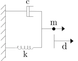
As an example, a simple mass-spring-damper shown in Figure 1 is represented by its state space model in Equations (7) and (8). While the system in this example is simple, and so is the

resulting state space model, complex models benefit immensely from the simple representation of first order differential equations during analysis and control design.

Figure 1: Example Mass-Spring-Damper System (image courtesy Aaron Yoon)

𝐴 = �_−𝑘0_{/𝑚 1/}1_𝑚� (7)

1.1.2.2 Lyapunov Stability

Aleksander Lyapunov developed a theory to determine stability of non-linear systems and published it in 1892. The theory found little use until the mid-1950’s when the technique was applied to non-linear control systems (specifically Sliding Mode Controllers discussed below) [2]. The theory can be broken into several components or definitions which are shown below.

Definition 1: The equilibrium state x = 0 is said to be stable if, for any R > 0, there exists r > 0, such that if ‖𝑥(0)‖ < r, then ‖𝑥(𝑡)‖ < R for all of t ≥ 0. Otherwise the equilibrium point is unstable.

Definition 1 is the broadest in terms of limiting a system. It states that if a state trajectory is started at a point located within a radius r of an equilibrium point and the state remains within the radius R of the equilibrium point for all of t > 0 it is stable.

Definition 2: An equilibrium point 0 is asymptotically stable if it is stable, and if in addition there exists some r > 0 such that ‖𝑥(0)‖ < r implies that x(t)  0 as t∞.

Definition 2 adds an additional restriction by defining the idea of asymptotic stability of a state. In this case if x(t)  0 as t∞, the equilibrium point is said to be asymptotically stable.

Definition 3: An equilibrium point 0 is exponentially stable if there exists two strictly positive numbers α and λ such that

∀𝑡> 0,‖𝑥(𝑡)‖ ≤ 𝛼‖𝑥(0)‖𝑒−𝜆𝑡 ₍₉₎

Definition 3 once again tightens the restrictions and states that for all times t > 0, that x(t) must not only approach zero, but that it must do it in an exponential fashion (its trajectory being bounded by 𝑒−𝜆𝑡 where λ is the rate of convergence).

Definition 4: A function, V(x), is said to be locally positive definite if V(0) = 0 and in a ball BR0

x ≠ 0 V(x) > 0. If V(0) = 0 and the above property holds over the entire state space, then V(x) is said to be globally positive definite.

Definition 5: If in a region defined by a ball BR0, the function V(x) is positive definite and has

continuous partial derivatives, and if its time derivative along any state trajectory of the system is negative semi-definite (𝑉̇(x) ≤ 0) then V(x) is said to be a Lyapunov function for the given system.

1.1.2.3 Sliding Mode Control

Sliding Mode Control was developed in the former USSR by several researchers [Aizerman and Gantmacher (1957), Emelyanov (1957), and Filippov (1960)] [2] during the 1950’s and 60’s and has continued to be an active area of research across several fields. [3] Some of its benefits include ease of application to a wide variety of typically difficult problems in controls such as nonlinear, MIMO, and large scale systems. Additionally, the method exhibits limited sensitivity to uncertainties (both intentionally un-modeled as a simplification, and un-known), and external disturbances assuming the bounds of these uncertainties are known. Along with these superior noise rejection capabilities, it also lends itself to state-space models providing the designer with a straightforward integration path. [3]

Drawbacks include the difficulty of inverting a non-square input influence matrix (also known as the B matrix). If the number system inputs do not match the system order, the matrix will be non-square. Non-square input influence matrices occur often in real world systems, especially in aircraft which commonly include redundant actuators and control paths. An additional drawback is the tendency of the controller to chatter, switching at a high rate, and potentially exciting undesired responses in the system under control. Chattering can be minimized, however, through various techniques such as a low pass filter on the output. [2]

As an example of a sliding mode controller consider the simple rotational system shown below: [3]

𝐽𝜃̈(𝑡) =𝑢(𝑡) (10)

Where:

𝐽= 𝑖𝑛𝑒𝑟𝑡𝑖𝑎𝑚𝑜𝑚𝑒𝑛𝑡 𝜃̈(𝑡) =𝑎𝑛𝑔𝑙𝑒𝑠𝑖𝑔𝑛𝑎𝑙 𝑢(𝑡) = 𝑐𝑜𝑛𝑡𝑟𝑜𝑙𝑖𝑛𝑝𝑢𝑡

(11)

The sliding surface is defined as:

𝑠(𝑡) =𝑐𝑥(𝑡) +𝑥̇(𝑡) (12)

Where:

𝑐 > 0 (13)

The tracking error function and the related derivatives are defined as:

𝑥(𝑡) =𝜃(𝑡)− 𝜃𝑑(𝑡) (15)

𝑥̇(𝑡) =𝜃̇(𝑡)− 𝜃̇𝑑(𝑡) (16)

𝑥̈(𝑡) =𝜃̈(𝑡)− 𝜃̈𝑑(𝑡) (17)

Where θ, θd, and their related derivatives are the actual and desired angular positions, velocities,

and accelerations.

Taking the derivative of the sliding function (ensuring no movement of the state error trajectories is allowed once the trajectories reach the sliding surface) and substituting the error functions yield:

𝑠̇(𝑡) =𝑐𝑥̇(𝑡) +𝑥̈(𝑡) (18) 𝑠̇(𝑡) =𝑐𝑥̇(𝑡) +𝜃̈(𝑡)− 𝜃̈𝑑(𝑡) (19)

𝑠̇(𝑡) =𝑐 �𝜃̇(𝑡)− 𝜃̇𝑑(𝑡)�+𝜃̈(𝑡)− 𝜃̈𝑑(𝑡) (20)

𝑠̇(𝑡) =𝑐 �𝜃̇(𝑡)− 𝜃̇𝑑(𝑡)�+1_{𝐽 𝑢}(𝑡)− 𝜃̈𝑑(𝑡) (21)

To ensure the Lyapunov stability (discussed in Section 1.1.2.2) of the function being positive, and the derivatives being negative, the following criteria must be met:

𝑠𝑠̇< 0 (22)

1

2𝑠2 ≥ 0 (23)

By substitution of the previous equations:

𝑠𝑠̇ =𝑠 �𝑐�𝜃̇ − 𝜃̇𝑑�+1_{𝐽 𝑢 − 𝜃}̈𝑑� (24)

Solving for u(t), the controller becomes:

𝒖(𝑡) =𝐽�𝑐�𝜃̇ − 𝜃̇𝑑�+𝜃̈𝑑− 𝜂𝑠𝑖𝑔𝑛(𝑠)� (25)

𝑠𝑖𝑔𝑛(𝑠) =� 1,0,𝑠𝑠 > 0= 0

−1,𝑠 < 0

Background work

2

Combining state space models with sliding mode controllers provides the unique opportunity to handle MIMO control cases and achieve near perfect tracking of the selected states. Typically, however, the requirement exists that the input influence matrix be square (where the number of inputs is equal to the number of system states). Literature on the topic of dynamic inversion is available in a broad array of application areas, however, none make the novel leap to include control effort, MIMO systems, and control allocation in the derivation of the solution.

An example of aircraft applications include a dynamic inversion paper by Enns et al in 1994 [4] where the technique was applied to an F18 with the authors even noting the fact that the input influence matrix could be badly conditioned for the technique. The issue was avoided by not solving that case. Over time techniques have appeared expanding the range of problems and methods used such as in the more recent paper by Hameduddin in 2011 [5] which applied the method to aircraft trajectory tracking. Hameduddin et al relied on the Moore-Penrose (discussed in Section 3.1.1) inverse to address the non-square input influence matrix of a MIMO system, and was thus unable to take into account control effort or state tracking selection. Aside from the papers of [6] [7] who themselves expressed the lack of documented work in using a technique such as this, there is little references in the transformation matrix technique discussed herein.

2.1 Non-Square Systems

In real world systems it is exceedingly rare to find a system in which the number of system inputs matches the system order. As mentioned previously, systems such as aircraft (both high performance and commercial) typically include redundant control actuators. The situation alone can create a case where the number of system states exceeds the number of system inputs. In these types of scenarios (and others, as both under- and over-actuated systems exhibit this issue) an inversion of a non-square B matrix to derive the Sliding Mode Control solution is required.

2.1.1 Moore-Penrose Pseudo-inverse

Mathematical solutions for inverting non-square matrices do exist in common practice and domain specific literature, however none address all of the desired requirements when inverting to implement a Sliding Mode Controller. The most common solution used in literature is the Moore-Penrose pseudo-inverse. [8] [9] While this solution does share some of the properties of a true inverse and can be used in the implementation of a Sliding Mode Controller, the suboptimal technique does not provide a method to target desired states for tracking purposes, and/or

minimize cost in terms of controller effort. In fact its tracking ability is limited to the actuated states only. [7]

2.1.2 Dynamic Extension

Dynamic extension is another technique capable of modifying a system such that the input influence B matrix is squared through a transformation. While the method is capable of

calculating the dynamic extension becomes impractical for systems exceeding 2 or 3 states and likely explains its rarity in published literature [2] .

2.1.3 Current Effort – Squaring Transformation Matrix

Most recent solutions in the development of a squaring transformation matrix technique were developed by Schkoda, DiFiore, and Crassidis; with extension to MIMO systems. Schkoda’s research was concerned with the development of a controller for non-square SISO under actuated systems. DiFiore’s work used the case of actuators being equal to the number of states to

collapse the problem to a SISO solution. While these developments were progressions towards applications on some real world systems (leaving behind pseudo-inverse techniques and applying it to fuel cell control problem) the existing solutions did not address the case of multiple system inputs where actuators do not match the state count. This limits the applicability of this technique on real world systems (e.g. aircraft which implement redundant actuators) until the extension is made. Both Schkoda and DiFiore proposed future efforts in developing the extension attempted herein.

To develop and demonstrate the extension to MIMIO systems the following steps were taken:

1. Research existing methods to understand the theoretical fundamentals of the square and under-actuated dynamic inversion solutions

2. Examine the theoretical solution for under-actuated systems by mathematically extending existing techniques to MIMO problems while retaining the control allocation and effort considerations

Theoretical Development

3

3.1 Squaring Transformation Matrix for Under Actuated Systems

None of above techniques includes a cost function into their computations making them difficult to implement directly in real world applications allowing for control allocation and tracking of selectable state. For example the current solutions do not take into account the range of an actuator, control surface loading, and available power; nor do current solutions attempt to minimize the control displacement and its impact on rate and position saturation. [6]

Additionally, the Moore-Penrose pseudo inverse does not allow for control allocation of system actuators at all.

Schkoda, whose paper and thesis were the inspiration for this research, developed a method to compute a transformation matrix to ‘square up’ the input influence matrix for the purposes of solving the sliding mode controller equations. The initial derivation is briefly summarized below. [6]

Given a system defined by:

𝑥̇= 𝑨𝒙+𝑩𝒖 (27)

Where:

𝑨 ∈ ℝ𝑛𝑥𝑛 ₍₂₈₎

𝑩 ∈ ℝ𝑛𝑥1 ₍₂₉₎

Note that B is non-square in the case of an under- or over-actuated system. Define the sliding surface as:

𝑠= 𝒙 − 𝒙𝒅+γ� (𝒙 − 𝒙𝒅)𝑑𝑟 𝑡

0

(30)

Take the derivative and set the result equal to 0:

𝑠̇ =𝒙̇ − 𝒙𝒅̇ +γ𝒙�= 0 (31)

Substituting the original state space model into this equation yields:

0 = 𝐴𝒙+𝐵𝒖 − 𝒙̇𝒅+γ𝒙� (32)

𝒖=𝑩−1_[𝑥̇

𝑑− 𝑨𝒙 −γ𝑥�] (34)

Therefore the input influence matrix (or B matrix) must be inverted to solve for the control effort. Schkoda [6] proposed a coordinate transformation such that the transformed system would result in a square (and thus invertible) system by defining the following transformation:

𝑦 =𝑻𝑥 (35)

Where:

𝑻 ∈ ℝ1𝑥𝑛 ₍₃₆₎

Note that the dimensions of T are the transpose of B.

Differentiating the transformation and substituting it into the original state space equation yields:

𝒚̇=𝑻𝒙̇ → 𝒙̇= 𝑨𝑥+𝑩𝑢 (37) 𝒚̇= 𝑻[𝑨𝒙+𝑩𝒖] =𝑻𝑨𝒙+𝑻𝑩𝒖 (38)

A new sliding surface is defined as:

𝒔=𝒚 − 𝒚𝒅+γ�(𝒚 − 𝒚𝒅)𝑑𝑟 𝑡

0

(39)

Differentiating the sliding surface and setting it equal to zero once again (utilizing Leibniz’s Rule [10] which allows us to move the differential through the integral insert the limits):

𝒔̇= 𝒚̇ − 𝒚𝒅̇ +γ𝒚�= 0 (40)

Substituting our updated state space equation into our sliding surface equation yields:

𝑻𝑨𝒙+𝑻𝑩𝒖 − 𝒚𝒅̇ +γ𝒚�= 0 (41)

𝑻𝑩𝑢 = 𝒚𝒅̇ − 𝑻𝑨𝑥 −γ𝒚�= 0 (42)

𝒖= (𝑻𝑩)−1_[𝒚̇

Note again that the choice of T will result in TB being square, thus as mentioned above:

𝑻 ∈ ℝ𝑚𝑥𝑛 ₍₄₄₎

The problem now reduces to finding T such that its dimensions are the transpose of B’s, where the tracking of selectable states is possible, and minimization of the control effort required. A possible solution is to employ a Linear Quadratic Regulator (LQR) cost function used

extensively in optimal control problems to find an “optimal” T for the selection of desirable tracking states and including allocation of the control effort:

𝐽 =1₂𝒙𝑇_�𝑡

𝑓�𝑆𝒙�𝑡𝑓�+1₂� (𝑥𝑇𝑸𝑥+𝑢𝑇𝑹𝒖)𝑑𝑡 𝑡𝑓

𝑡0

(45)

Q is chosen to weight the states the designer desires to track, and R is used to allocate the control effort. The standard LQR solution in optimal control has the following control feedback form for the control effort:

𝒖= −𝑲𝒙 (46)

Substitute the previous equation into the following and solve for T:

𝒖=−(𝑻𝑩)−1_{𝑻[𝑨+γ𝑰]𝒙} (47) 𝑲= (𝑻𝑩)−1_{𝑻[𝑨+γ𝑰]} (48) 𝑻 = (𝑻∗𝑩)𝑲(𝑨+γ𝑰)−1 (49)

Where:

𝑻∗ = 𝑩𝑇 (50)

Substituting T back into our control law equation yields:

𝒖= (𝑻∗𝑩)−1𝑻[𝒙̇𝒅− 𝑨𝒙 −γ𝒙�] (51)

problem reduced to a SISO type system once again. [7] As demonstrated in the example below, the proposed technique can be extended to under-actuated systems with multiple inputs while maintaining the control allocation and effort benefits.

3.2 MIMO Derivation

Below is the re-derivation of the above technique to address MIMO systems.

Given a system defined by:

𝒙̇= 𝑨𝒙+𝑩𝒖 (52)

Where:

𝑨 ∈ ℝ𝑛𝑥𝑛 (53)

𝑩 ∈ ℝ𝑛𝑥𝑚 (54)

Note B is defined to be non-square as in the case of an under- or over-actuated system and in this case m is greater than 1.

Define the sliding surface as before:

𝑠= 𝒙 − 𝒙𝒅+γ� (𝒙 − 𝒙𝒅)𝑑𝑟 𝑡

0

(55)

Take the derivative and setting the result equal to zero ensures no movement of the state tracking error dynamics once the trajectories reach the sliding surface and yields:

𝒔̇= 𝒙̇ − 𝒙𝒅̇ +γ𝒙� = 0 (56)

Inputting the state space model into the SMC equations yields:

0 = 𝑨𝒙+𝑩𝒖 − 𝒙̇𝒅+γ𝒙� (57)

−𝑨𝒙+𝒙̇𝒅−γ𝒙� =𝑩𝒖 (58)

𝒖=𝑩−1_[𝒙̇

Once again, as anticipated; the inversion of the input influence B matrix is required. Defining a coordinate transformation as follows:

𝒚=𝑻𝒙 (60)

Where:

𝑻 ∈ ℝ𝑚𝑥𝑛 ₍₆₁₎

Noting that the dimensions of T are the transpose of B, and m is greater than 1. Differentiating T and substituting it into the original state space equation yields:

𝒚̇= 𝑻𝒙̇ → 𝒙̇=𝑨𝒙+𝑩𝒖 (62) 𝒚̇= 𝑻[𝑨𝒙+𝑩𝒖] =𝑻𝑨𝒙+𝑻𝑩𝒖 (63)

A new sliding surface can be defined as:

𝒔=𝒚 − 𝒚𝒅+γ�(𝒚 − 𝒚𝒅)𝑑𝑟 𝑡

0

(64)

Differentiating Eq. (64) and setting it equal to zero once again (utilizing Leibniz’s Rule [10]):

𝒔̇= 𝒚̇ − 𝒚𝒅̇ +γ𝒚�= 0 (65)

Finally, inserting the new state space equation into the sliding surface equation yields:

𝑻𝑨𝒙+𝑻𝑩𝒖 − 𝒚𝒅̇ +γ𝒚�= 0 (66)

𝑻𝑩𝑢 =𝒚𝒅̇ − 𝑻𝑨𝒙 −γ𝒚�= 0 (67)

𝒖= (𝑻𝑩)−1_[𝒚̇

𝒅− 𝑻𝑨𝒙 −γ𝒚�] (68)

Note: With B having m greater than 1, the product of TB will remain square due to the selection of T as the transpose of B:

The problem now reduces to finding a T such that the dimensions of T are the transpose of B’s, near perfect tracking at desired selectable states is achieved, and control effort is minimized through control allocation. Choosing T such that the LRQ cost function is minimized (assuming a linearized plant):

𝐽= 1₂𝑥𝑇_�𝑡

𝑓�𝑆𝑥�𝑡𝑓�+1₂� (𝑥𝑇𝑸𝑥+𝑢𝑇𝑹𝑢)𝑑𝑡 𝑡𝑓

𝑡0

(70)

Choosing Q in such that the desired states to track are weighted, and R to allocate the control effort, the standard LQR problem can be solved for the feedback gain matrix K:

𝒖= −𝑲𝒙 (71)

Substituting into our control equation and solving for T:

𝒖=−(𝑻𝑩)−1_{𝑻[𝑨+γ𝑰]𝒙 (72)}

𝑲= (𝑻𝑩)−1_{𝑻[𝑨+γ𝑰] (73)}

𝑻 = (𝑻∗𝑩)𝑲(𝑨+γ𝑰)−1 (74)

Where:

𝑻∗ = 𝑩𝑇 (75)

Substituting T back into our original control law equation:

𝒖= (𝑻∗𝑩)−1𝑻[𝒙̇𝒅− 𝑨𝒙 −γ𝒙�] (76)

Results

4

To demonstrate the effectiveness of the newly derived control technique, several simulations were developed to model the system responses, and quantify the resulting performance. The Moore-Penrose inverse was used as the baseline or legacy technique. These simulations were performed on a four-mass-spring-damper problem and a longitudinal aircraft model. The primary control objective undertaken in these simulations was, given a set of desired states; track one of the non-directly actuated states, with the minimum control effort.

4.1 Under-Actuated System Example

To demonstrate the technique a derivation and results of the technique discussed previously the method is applied to a basic 4 mass-spring-damper system with two force inputs. A diagram showing the system is presented in Figure 2 below.

Figure 2: Four Mass-Spring-Damper System (image courtesy Markus Kottmann)

4.1.1 System Assumptions

Input forces:

𝒖= [𝑢1𝑢2] (77)

Four positions and four velocities as outputs (which match the internal states below):

𝒚= [𝑦1𝑦2𝑦3𝑦4𝑦1̇ 𝑦2̇ 𝑦3̇ 𝑦4̇] (78)

State variables are assumed to be:

𝑥1 =𝑦1

𝑥2 = 𝑦2

𝑥3 = 𝑦3

𝑥4 = 𝑦4

𝑥5 = 𝑦1̇

𝑥6 = 𝑦2̇

𝑥7 = 𝑦3̇

𝑥8 = 𝑦4̇

Physical constants are given as:

𝑚 = 1𝑘𝑔 𝑘 = 36_𝑚𝑁

𝑏 = 0.6𝑁 ∙ 𝑠_𝑚

(80)

4.1.2 State Space Model Derivation

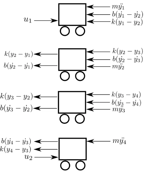
Starting from the system model shown in Figure 2 above, the state space model was derived in the process shown below.

Figure 3: Free-body diagrams for four mass-spring-damper system

Using Lagrange’s energy method to compute the equations of motion the system is described via a set of energy equations [11].

With the kinetic energy elements of the system represented by T:

𝑇=1₂𝑚𝑦̇12+1₂𝑚𝑦̇22 +1₂𝑚𝑦̇32+1₂𝑚𝑦̇42 (81)

And the potential energy elements represented by V:

𝑉= 1₂𝑘(𝑦2 − 𝑦1)2+1₂𝑘(𝑦3− 𝑦2)2+1₂𝑘(𝑦4− 𝑦3)2 (82)

Solving for the Lagrangian representation, denoted by L:

𝐿=𝑇 − 𝑉 (83)

−1₂𝑘(𝑦2− 𝑦1)2−1₂𝑘(𝑦3− 𝑦2)2−1₂𝑘(𝑦4− 𝑦3)2

Computing the Rayleigh dissipation elements, denoted by R:

𝑅 = 1₂𝑏(𝑦̇2− 𝑦̇1)2+1₂𝑏(𝑦̇3− 𝑦̇2)2+1₂𝑏(𝑦̇4− 𝑦̇3)2 (85)

Given the Lagrange equation below:

𝐹𝑞𝑖 =

𝑑 𝑑𝑡 �

𝜕𝐿 𝜕𝑞𝚤̇ � −

𝜕𝐿 𝜕𝑞𝑖 +

𝜕𝑅

𝜕𝑞𝚤̇ (86)

By substitution and differentiation, the four equations of motion are found to be:

𝑚𝑦1̈ − 𝑘(𝑦2− 𝑦1)− 𝑏(𝑦2̇ − 𝑦1̇ ) =𝑢1 (87)

𝑚𝑦2̈ +𝑘(𝑦2− 𝑦1)− 𝑘(𝑦3− 𝑦2) +𝑏(𝑦2̇ − 𝑦1̇ )− 𝑏(𝑦3̇ − 𝑦2̇ ) = 0 (88)

𝑚𝑦3̈ +𝑘(𝑦3− 𝑦2)− 𝑘(𝑦4− 𝑦3) +𝑏(𝑦3̇ − 𝑦2̇ )− 𝑏(𝑦4̇ − 𝑦3̇ ) = 0 (89)

𝑚𝑦4̈ +𝑘(𝑦4− 𝑦3) +𝑏(𝑦4̇ − 𝑦3̇ ) =𝑢2 (90)

Solve for the eight state equations:

𝑥1̇ = 𝑦1̇ =𝑥5 (91)

𝑥2̇ =𝑦2̇ =𝑥6 (92)

𝑥3̇ =𝑦3̇ =𝑥7 (93)

𝑥4̇ =𝑦4̇ =𝑥8 (94)

𝑥5̇ =𝑦1̈ = −_𝑚𝑏(𝑦1̇ − 𝑦2̇ )−_𝑚𝑘 (𝑦1− 𝑦2) +𝑢_𝑚1 (95)

𝑥6̇ =𝑦2̈ =−_𝑚𝑘 (𝑦2− 𝑦1)−_𝑚𝑏 (𝑦2̇ − 𝑦1̇ )−_𝑚𝑘 (𝑦2− 𝑦3)−_𝑚𝑏 (𝑦2̇ − 𝑦3̇ ) (96)

𝑥7̇ =𝑦3̈ =−_𝑚𝑏 (𝑦3̇ − 𝑦2̇ )−_𝑚𝑘(𝑦3− 𝑦2)−_𝑚𝑏 (𝑦3̇ − 𝑦4̇ )−_𝑚𝑘 (𝑦3− 𝑦4) (97)

Rearranging yields:

𝑥5̇ =_𝑚1[−𝑘𝑥1+𝑘𝑥2− 𝑏𝑥5+𝑏𝑥6+𝑢1] (99)

𝑥6̇ =_𝑚1[𝑘𝑥1− 𝑘𝑥2 − 𝑘𝑥2+𝑘𝑥3 +𝑏𝑥5 − 𝑏𝑥6− 𝑏𝑥6+𝑏𝑥7] (100)

𝑥7̇ =_𝑚1[𝑘𝑥2− 𝑘𝑥3− 𝑘𝑥3 +𝑘𝑥4+𝑏𝑥6− 𝑏𝑥7− 𝑏𝑥7+𝑏𝑥8] (101)

𝑥8̇ =_𝑚1[𝑘𝑥3− 𝑘𝑥4+𝑏𝑥7− 𝑏𝑥8+𝑢2] (102)

Formatting the above state equations into standard state space matrix format yields:

𝑨= ⎣ ⎢ ⎢ ⎢ ⎢ ⎢ ⎢ ⎢ ⎢ ⎢ ⎢ ⎢

⎡ 0₀ 0₀ 0₀ 0₀ 1₀ 0_{1 0}0 0₀

0 0 0 0 0 0 1 0

0 0 0 0 0 0 0 1

−_𝑚𝑘 _𝑚𝑘 0 0 −_𝑚𝑏 _𝑚𝑏 0 0

𝑘

𝑚 −2∗ 𝑘 𝑚

𝑘

𝑚 0

𝑏

𝑚 −2∗ 𝑏 𝑚

𝑏

𝑚 0

0 _𝑚𝑘 −2∗_𝑚𝑘 _𝑚𝑘 0 _𝑚𝑏 −2∗_𝑚𝑏 _𝑚𝑏

0 0 _𝑚𝑘 −_𝑚𝑘 0 0 _𝑚𝑏 −_𝑚⎦𝑏⎥

⎥ ⎥ ⎥ ⎥ ⎥ ⎥ ⎥ ⎥ ⎥ ⎥ ⎤ (103) 𝑩= ⎣ ⎢ ⎢ ⎢ ⎢ ⎢ ⎢ ⎢ ⎢ ⎡0 0_{0 0}

0 0 0 0 1 𝑚 0 0 0 0 0 0 _𝑚⎦1⎥

⎥ ⎥ ⎥ ⎥ ⎥ ⎥ ⎥ ⎤ (104) 𝑪= ⎣ ⎢ ⎢ ⎢ ⎢ ⎢ ⎢

⎡1 0 0 0 0 0 0 0_{0 1 0 0 0 0 0 0} 0 0 1 0 0 0 0 0 0 0 0 1 0 0 0 0 0 0 0 0 1 0 0 0 0 0 0 0 0 1 0 0 0 0 0 0 0 0 1 0

0 0 0 0 0 0 0 1⎦⎥

𝑫= ⎣ ⎢ ⎢ ⎢ ⎢ ⎢ ⎢ ⎡0 0_{0 0}

0 0 0 0 0 0 0 0 0 0 0 0⎦⎥

⎥ ⎥ ⎥ ⎥ ⎥ ⎤ (106)

4.1.3 Pseudo-Inverse Controller

Given the state space system defined previously in Equations (103) – (106) of the form:

𝒙̇= 𝑨𝒙+𝑩𝒖 (107)

Where:

𝑨 ∈ ℝ8𝑥8 (108)

𝑩 ∈ ℝ8𝑥2 (109)

Note: B is defined to be non-square as in the case of an under- or over-actuated system and in this case m is 2.

Define the sliding surface as before (see Equation (30)):

𝑠= 𝒙 − 𝒙𝒅+γ� (𝒙 − 𝒙𝒅)𝑑𝑟 𝑡

0

(110)

Take the derivative and setting the result equal to zero yields:

𝒔̇= 𝒙̇ − 𝒙𝒅̇ +γ𝒙� = 0 (111)

Inputting the state space model into the SMC equations yields:

0 = 𝑨𝒙+𝑩𝒖 − 𝒙̇𝒅+γ𝒙� (112)

−𝑨𝒙+𝒙̇𝒅−γ𝒙� =𝑩𝒖 (113)

𝒖= 𝑩−1_[𝒙̇

𝒅− 𝑨𝒙 −γ𝒙�] (114)

The MATLAB implementation of the controller is formed as shown in Equation (115):

𝒖= −𝑝𝑖𝑛𝑣𝑒𝑟𝑠𝑒(𝑩)∗[(𝑨+γ∗ 𝑰)𝒙 −(𝛾 ∗ 𝒙𝒅)− 𝒙𝒅̇ ] (115)

The controller is then realized in the Simulink model as shown in Figure 4:

Figure 4: Four Mass Spring Damper Simulink Pseudo-Inverse Controller Model

4.1.4 Transformed Matrix Controller

Where:

𝑻∗ = 𝑩𝑇 (116)

Solving for T based on the derivation shown in Section 3.2 above. K is the gain matrix found by solving the standard LQR problem with the following inputs. Parameter gamma and matrix R are selected by starting with values used in previous research papers in this area, in combination order of magnitude LQR parameter selection techniques. Q is selected such that the desired control allocation state is several orders of magnitude above the remaining states. In the current example, it can be seen that to track Cart 3’s position Q[3,3] is set to 1,000,000,000, while the remainder of the matrix is the identity matrix. To track Cart 2’s position, Q[2,2] would be set similarly. This selection may be made for any of the 8 available states.

𝑸𝐶𝑎𝑟𝑡2𝑃𝑜𝑠𝑖𝑡𝑖𝑜𝑛 = ⎣ ⎢ ⎢ ⎢ ⎢ ⎢ ⎢

⎡1_{0 1000000000 0 0 0 0 0 0}0 0 0 0 0 0 0

0 0 1 0 0 0 0 0

0 0 0 1 0 0 0 0

0 0 0 0 1 0 0 0

0 0 0 0 0 1 0 0

0 0 0 0 0 0 1 0

0 0 0 0 0 0 0 1⎦⎥

⎥ ⎥ ⎥ ⎥ ⎥ ⎤ (117)

𝑸𝐶𝑎𝑟𝑡3𝑃𝑜𝑠𝑖𝑡𝑖𝑜𝑛 =

⎣ ⎢ ⎢ ⎢ ⎢ ⎢ ⎢

⎡1 0_{0 1} 0₀ 0 0 0 0 0_{0 0 0 0 0}

0 0 1000000000 0 0 0 0 0

0 0 0 1 0 0 0 0

0 0 0 0 1 0 0 0

0 0 0 0 0 1 0 0

0 0 0 0 0 0 1 0

0 0 0 0 0 0 0 1⎦⎥

⎥ ⎥ ⎥ ⎥ ⎥ ⎤ (118)

𝑹= � 10 0_{0 10}� (119)

𝛾 = 20 (120)

Substitute the resulting K (feedback gain matrix) obtained via MATLAB’s lqr()function into the earlier derived formula for T:

𝑻= 𝑻∗𝑩𝑲[𝑨+𝛾 ∗ 𝑒𝑦𝑒(8)]−1 𝑦𝑖𝑒𝑙𝑑𝑠

�⎯⎯⎯�

𝑻= �_{0.5329 34.9241 429.1039 35.4328}0.6738 −1.3278 −1.0004 −0.8526 ₋0.1536_{0.0169 0.6982 18.8197 0.6807}0.0422 −0.2322 0.0833�(121)

The following equation is realized in Simulink as shown in Figure 5:

Figure 5: Four Mass Spring Damper Transformed Matrix Simulink Model

4.1.5 Results and Comparison of Techniques

Given the Simulink model described in Section 4.1.4, numerical simulations were ran to

establish the system response and controller performance for both discussed techniques. In these simulations, a target state was selected to optimize tracking of. While all states were simulated, a representative example, State Three (Cart Three’s position), is examined here. Shown in Figure 6 (and Figure 8), the tracking of State Three was nearly perfect and State Four had minimal error when controlled with the transformed matrix technique. While this transformed matrix control methodology did not exhibit particularly good performance in tracking States One and Two, they were not targeted during the system design so this is to be expected. The tracking of these non-primary states can likely be tuned via optimization of Q matrix value selection.

Figure 6: Transformed Matrix Tracking Results

Figure 8: Tracking Error

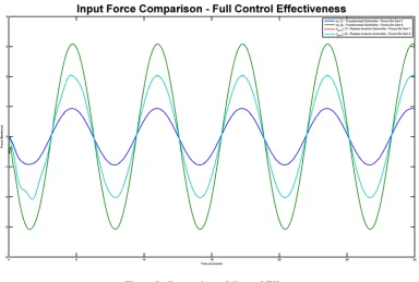
Figure 9: Comparison of Control Effort

In addition to the simulation of State Three, shown above, States One, Two, and Four were also simulated. The resulting tracking accuracy and control effort are then rolled up via cost functions into performance metrics. These numbers allowed direct comparison between the two techniques across all four simulations.

The cost function used to characterize control effort is shown in Equation (123). The lower the resulting number, the less control effort was demanded by the controller:

𝑎𝑣𝑒𝑟𝑎𝑔𝑒𝑐𝑜𝑛𝑡𝑟𝑜𝑙𝑒𝑓𝑓𝑜𝑟𝑡 =� ���30|𝑢|𝑑𝑡

0 �/30�

(123)

Realized in MATLAB functions as:

𝑐𝑜𝑛𝑡𝑟𝑜𝑙𝑒𝑓𝑓𝑜𝑟𝑡= 𝑠𝑢𝑚(𝑡𝑟𝑎𝑝𝑧(𝑎𝑏𝑠(𝑢)./𝑡𝑖𝑚𝑒(𝑒𝑛𝑑)) (124)

The cost function for tracking accuracy is shown in Equation (125). The lower the resulting number, the better the tracking:

In MATLAB the syntax below was used. Of note eps() was added to xi to prevent divide by

zero errors:

𝑡𝑟𝑎𝑐𝑘𝑖𝑛𝑔𝑎𝑐𝑐𝑢𝑟𝑎𝑐𝑦=𝑠𝑢𝑚(𝑎𝑏𝑠(𝑥𝑑𝑖_𝑥− 𝑥𝑖

𝑖 +𝑒𝑝𝑠)) (126)

The previous metrics were then used to track each controller’s response at tracking each state. Control effort is shown below in Table 1 and the tracking effort is shown in Table 2. It becomes readily apparent in Table 2 that the tracking accuracy how the new method outperformed the legacy technique. On all four trials its tracking accuracy far exceeded the Moore-Penrose method. In terms of control effort, simulations on States Three and Four showed higher control effort, but as discussed previously, is acceptable since tracking accuracy is significantly

improved over the alternative. Of note, the control effort did not change for any of the legacy pseudo inverse simulations as the technique does not adjust its control methodology for various states.

Table 1: Mass-Spring-Damper Control Effort Comparison

State Number State

Description

Average Control Effort T-Matrix

Average Control Effort P-Inverse

1 Cart 1 Position 2665.2 9890.8

2 Cart 2 Position 10318.5 9890.8

3 Cart 3 Position 9515.7 9890.8

4 Cart 4 Position 867.4 9890.8

Table 2: Mass-Spring-Damper Tracking Accuracy Comparison

State Number State

Description

Average Tracking Accuracy T-Matrix

Average Tracking Accuracy P-Inverse

1 Cart 1 Position 1146.2 45382.3

2 Cart 2 Position 4562.0 19034.7

3 Cart 3 Position 6288.6 17726.6

4 Cart 4 Position 3811.3 40460.3

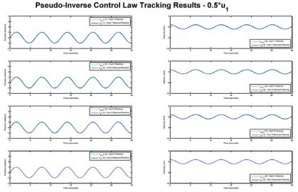
4.1.6 Control Allocation

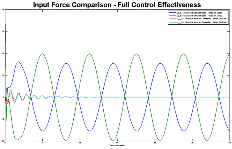
To demonstrate the control allocation properties of the technique a 0.5 scaling gain was applied to one of the input force terms. As shown in the plots below, the controller experienced minimal performance impact other than the additional control effort bourn by the remaining

Figure 10: Four Mass Spring Damper – Transformed Matrix - Control Allocation

Figure 12: Tracking Error - Control Allocation

Figure 13: Control Effort - Control Allocation

While tracking error increases for the non-selected states (shown in Figure 15), and control effort used is higher (shown in Figure 16), the tracking remains near perfect for the selected state.

Figure 14: Non-Optimal Input - Tracking Results

Figure 16: Non-Optimal Input - Control Effort

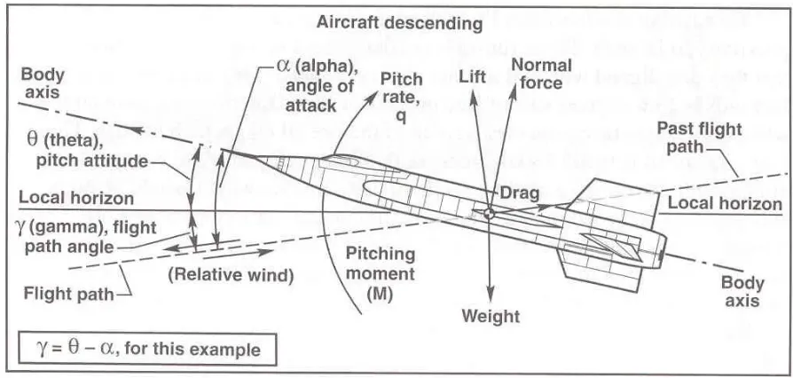
4.2 Longitudinal Aircraft Model

This model is representative of a high performance jet aircraft and provides an opportunity to demonstrate the controller performance in a real world application. For sake of clarity, the model has been limited to only its longitudinal states which consist of velocity (Vt), flight path angle

Figure 17: Longitudinal Terms of a Climbing Aircraft (image courtesy of NASA OLD)

Figure 18: Longitudinal Terms of a Descending Aircraft (image courtesy of NASA OLD)

4.2.1 Pseudo-Inverse Controller

Figure 19: Legacy Implementation

𝑢 = − 𝑝𝑖𝑛𝑣(𝐵)∗[(𝐴+𝛾 ∗ 𝐼)𝑥 −(𝛾 ∗ 𝑥𝑑)− 𝑥𝑑̇ ] (127)

Figure 20: Moore-Penrose Pseudo-Inverse Controller

4.2.2 Transformed Matrix Controller

The transformed matrix controller Simulink implementation is shown in Figure 21 below. The details of the implementation are highlighted in Figure 22 and rely on the MATLAB standard matrix inverse (suitable for square matrices) inv()applied to the product of B and its

Figure 21: Transformed Matrix Simulink Implementation

𝑢 = − 𝑖𝑛𝑣(𝑇∗∗ 𝐵)𝑇 ∗[(𝐴+𝛾 ∗ 𝐼)𝑥 −(𝛾 ∗ 𝑥𝑑)− 𝑥𝑑̇] (128)

Figure 22: Transformed Matrix Implementation Detail

4.2.3 Results and Comparison of Techniques

To analyze the performance of the expanded transformation technique, it was applied to the previously discussed longitudinal aircraft model across three sets of simulations including:

• Nominal operation – Demonstrate the suitability of the derived controller to the example system (a longitudinal aircraft model) and its performance compared to the Moore-Penrose pseudo-inverse method.

• Wind gusts – Demonstrate that the derived controller retains the external disturbance rejection capability of the standard sliding mode controller, and outperforms the Moore-Penrose pseudo-inverse method in disturbance laden environments.

4.2.3.1 Nominal Response

The system was simulated for 30 seconds with the desired state inputs being a sine wave at 1 rad/sec for states 1 and 3, and negative cosine at 1 rad/sec for states 2 and 4. The transformation matrix inversion technique was setup to optimize tracking of state 3 (flight path angle) in the Q matrix, and control allocated in the R matrix towards the elevator actuator.

Figure 23: Longitudinal Aircraft Model – Flight Path Tracking

Figure 24: Longitudinal Aircraft Model – Flight Path Tracking – Tracking Error

The error plot in Figure 24 better shows the resulting tracking differences between the

techniques. In terms of tracking a non-directly connected state, in this case tracking State Two, the transformed matrix technique is superior to the legacy pseudo-inverse method.

In terms of control effort, the legacy method primary uses the throttle, a non-ideal control method in this case, while the transformed matrix method uses the elevator. This is due to the small coupling term present in the input influence matrix that cannot be adjusted for in the legacy technique. The transformed matrix method can be weighted via the R matrix to account for this.

Figure 26: Longitudinal Aircraft Model – Control Deflections– Flight Path Tracking

Figure 26 shows the control deflections throughout the simulation. Quickly apparent is the movement of the throttle to track flight path, a non-optimal use of control effort.

Once again a set of cost functions were utilized to characterize the two controller’s performance across a set of state selections. Average control effort was defined again as below. Lower is better:

𝑎𝑣𝑒𝑟𝑎𝑔𝑒𝑐𝑜𝑛𝑡𝑟𝑜𝑙𝑒𝑓𝑓𝑜𝑟𝑡 =� ���30|𝑢|𝑑𝑡

0 �/30�

(129)

And implemented in MATLAB as:

𝑐𝑜𝑛𝑡𝑟𝑜𝑙𝑒𝑓𝑓𝑜𝑟𝑡= 𝑠𝑢𝑚(𝑡𝑟𝑎𝑝𝑧(𝑎𝑏𝑠(𝑢)./𝑡𝑖𝑚𝑒(𝑒𝑛𝑑)) (130)

The tracking accuracy metric is shown in Equation (131). Lower is better:

MATLAB implementation:

𝑡𝑟𝑎𝑐𝑘𝑖𝑛𝑔𝑎𝑐𝑐𝑢𝑟𝑎𝑐𝑦=𝑠𝑢𝑚(𝑎𝑏𝑠(𝑥𝑑𝑖_𝑥− 𝑥𝑖

𝑖 +𝑒𝑝𝑠)) (132)

The results from these sets of simulations are shown in the tables below. The comparison of control effort has two items of note. First the control effort for the pseudo-inverse does not change despite the change in desired state. This gives insight into the fact that the legacy method is unable specifically target a desired state. Secondly, the average control effort utilized by the transformed matrix method is significantly lower than the legacy method. Again, this is intuitive since the legacy method does not have a method minimize the utilized effort.

Table 3: Longitudinal Aircraft State Control Effort Comparison

State Number State

Description

Average Control Effort T-Matrix

Average Control Effort P-Inverse

1 Velocity 16.1 156.2

2 Flight Path 15.1 156.2

3 Pitch Rate 9.8 156.2

4 Pitch 9.9 156.2

The tracking accuracy comparison is mixed between the transformed matrix and legacy method. The pseudo-inverse has direct control of velocity and pitch rate and thus can exceed the tracking performance of the transformed matrix on those states. However, keep in mind that the legacy technique does not consider control effort, and with optimization of the Q matrix, improvement on those two states is likely achievable with minimal impact on overall system performance. The remaining states of flight path and pitch are tracked with significantly better accuracy with the transformed matrix method without any additional optimization of state weighting.

Table 4: Longitudinal Aircraft State Tracking Accuracy Comparison

State Number State

Description

Average Tracking Accuracy T-Matrix

Average Tracking Accuracy P-Inverse

1 Velocity 2050.3 560.9

2 Flight Path 3715.6 9234.8

3 Pitch Rate 794.3 125.4

4.2.3.2 Noise Rejection Properties

One of the benefits of utilizing a sliding mode controller is its rejection of external disturbances. The longitudinal aircraft model was again used to model the controllers ability to track a given flight path, however in this case a wind gust model was placed in-line with the state-space model output to model disturbances on the system. Given the variances listed in Table 5 below, and the Dryden Wind Model [U.S. Military Handbook MIL-HDBK-1797, 19 December 1997], the model was simulated for 30 seconds to track a given flight path, using the elevator as the primary control input.

Table 5: Wind Gust Variances

Parameter Variance

Vt_variance 0.1

gamma_variance 0.01

qb_variance 0.01

theta_variance 0.01

The Dryden gust model computed the α and Vt turbulences from the given variances and random

noise generators as shown in Figure 27 below. Figure 28 shows how the coupling between the gust model and the turbulence model was implemented.

Figure 28: Noise Injection Model

The flight path tracking results from both the transformed matrix and pseudo-inverse are documented below. The transformed matrix controller response, as expected, was exceptional; whereas the pseudo-inverse suffered significant lag and lacked the ability to track the input accurately (never approaching the desired path by more than 50%).

Figure 30: Longitudinal Aircraft Model – Pseudo-Inverse – Flight Path Tracking – Noise Rejection

Figure 31: Longitudinal Aircraft Model – Control Effort – Flight Path Tracking – Noise Rejection

4.2.3.3 Control Allocation

Demonstrated now is the control allocation properties of the technique. This allows a system designer to select a state to control in a system while minimizing the control effort required. This is of importance, for example, in situations where actuators may have failed, or suffer from reduced effectiveness. In the example below the longitudinal aircraft model discussed in Section 4.2 is again used. The tracking of a desired flight path using the elevator was demonstrated in Section 4.2.3.1. Here, tracking the flight path state is attempted using only the throttle (for example as in the event of a loss of control on an elevator). This is due to the (weak) link between flight path angle (γ) and throttle as seen in the system input influence matrix (B) [B(2,2)].

𝐵 =�

0.069 0.191 0.130 0.011

−9.383 0.039

0 0

� (133)

Recall the near perfect tracking of flight path with elevator control shown in Figure 23 and Figure 24 previously. The R matrix was reconfigured to force throttle control only, and is shown in Equation (134). The Q matrix remained the same as shown in the nominal example, setting the desired tracking state again to 2 (flight path angle).

𝑅 =�0.01_{0 1000}0 � (134)

Figure 33 shows an overlay of the desired tracking response and the actual system responses with the two controllers. The tracking performance of the legacy pseudo-inverse technique is subpar in comparison to the new transformation matrix. It is apparent that the legacy technique is unable to track flight path, with only directly connected states tracking with any accuracy.

Figure 33: Longitudinal Aircraft Model – Flight Path Tracking – Control Allocation

Figure 35: Longitudinal Aircraft Model – Control Effort – Flight Path Tracking – Control Allocation

Figure 37 below shows the near perfect tracking of flight path with throttle control only while the inability of the legacy technique to track a given flight path is shown; with only the directly connected states tracking with any accuracy. The transformed matrix technique does require additional control effort relative to the legacy method to achieve perfect tracking, however in real-world implementations this is often an acceptable trade-off. As shown in Figure 40 control chatter does not appear to be an issue in this case, however if noise were present in the system, mitigation techniques (such as low pass filters or saturation elements) may become required.

Figure 38: Longitudinal Aircraft Model –Flight Path Tracking Error Using Throttle Only

Figure 40: Longitudinal Aircraft Model – Flight Path Tracking Using Throttle Only – Control Deflections

In summary, the performance of the transformed matrix technique is superior to the legacy pseudo-inverse method in several areas. First, its tracking is often nearly perfect and nearly always at a lower control effort cost. Secondly, the control method provides for excellent

rejection of noise and modeling imperfections, assuming they are bounded. Third, control can be easily allocated by a system designer to address desired system performance traits, and/or

Conclusions

5

5.1 Conclusions

It has been demonstrated that among the methods to implement a dynamic inversion style

controller, commonly utilized methods have several shortcomings and the investigated technique addresses some of those shortcomings. The Moore-Penrose pseudo-inverse lacked the ability to select states to control other than those directly connected to the actuators. While dynamic extension can provide a solution to MIMO problems it lacks a general solution and therefore must be re-derived for every application and left the technique impractical to implement in practice. Schokda’s original squaring transformation matrix technique developed the initial use of the method on single input, linearized systems but did not demonstrate the control allocation properties of the technique, or situations where system noise was present. Finally, DiFiroe’s work addressed a specific class of nonlinear under actuated systems, using system order matching to collapse the problem match the SISO solution, again avoiding the over-actuated class of problems, and control allocation.

This thesis has demonstrated an extension of Shkoda’s transformation matrix technique to linearized MIMO systems. Through this effort the minimization of control effort, along with control allocation properties have been shown to perform as desired across two example

problems. Additionally, system noise was simulated on the longitudinal aircraft model, to which the derived controller showed excellent resistance. The results from both the four-mass-spring-damper and the longitudinal aircraft model simulations support the conclusion that the derived technique meets the desired performance goals.

5.2 Future Work

This thesis was focused on extending the discussed technique to MIMO systems and

demonstrating its performance compare to legacy techniques across several operational goals such as noise rejection, control effort, and control allocation properties, however the selection of parameters such as Q, R, in the LQR problem were not optimized. Future efforts could

investigate the optimal selection of these LQR parameters and how the parameters relate to system performance using techniques such as Monte Carlo simulations. Additionally, the optimization of γ in the SMC control function may provide opportunities for controller performance improvements.

Other areas for future research could seek to include more accurate actuator effects such as time delays into the system model and simulate the response and performance impact. Additionally, the method could be extended yet again to address non-linear systems and eventually

Societal Impact

6

References

7

[1] B. Friedland, Control System Design: An Introduction to State-Space Methods, McGraw-Hill, Inc., 2002.

[2] J.-J. E. Slotine and W. Li, Applied Nonlinear Control, Prentice-Hall, Inc., 1991.

[3] J. Liu and X. Wang, Advanced Sliding Mode Control for Mechanical Systems, Beijing: Tsinghua University Press (Springer), 2012.

[4] D. Enns, D. Bugajski, R. Hendrick and G. Stein, "Dynamic Inversion: An evolving methodology for flight control design," International Journal of Control, 1992.

[5] I. Hameduddin, "Generailized dynamic inversion for multiaxial nonlinear flight control," in

American Control Conference, San Francisco, 2011.

[6] R. Schkoda and A. Crassidis, "Dynamic Inversion Control for Non-Square Systems with Application to Aircraft Longitudinal Control," in AIAA Atmospheric Flight Mechanics Conference and Exhibit, Hilton Head, 2007.

[7] D. C. DiFiore, "Sliding Mode Control Applied to an Underactuated Fuel Cell System," Rochester, NY, 2009.

[8] R. Penrose, "A generalized inverse for matrices," Proceedings of the Cambridge Philosophical Society, vol. 51, pp. 406-413, 1955.

[9] E. H. Moore, "On the reciprocal of the general algebraic matrix," Bulletin of the American Mathematical Society, vol. 26, no. 9, pp. 394-395, 1920.

[10] R. Harron, "MAT-203: The Leibniz Rule," Boston.

[11] J. B. Tatum, Classical Mechanics, Victoria, 2013.

[12] W. J. Palm, System Dynamics, McGraw-Hill, Inc., 2004.

[13] E. Kreyszig, Advanced Engineering Mathematics, 2006: John Wiley & Sons.

[14] R. C. Nelson, Flight Stability and Automatic Control, McGraw-Hill, Inc., 1998.