A Neural Framework
for Low-Shot Learning
The Harvard community has made this
article openly available.
Please share
how
this access benefits you. Your story matters
Citable link
http://nrs.harvard.edu/urn-3:HUL.InstRepos:38811499
Terms of Use
This article was downloaded from Harvard University’s DASH
repository, and is made available under the terms and conditions
applicable to Other Posted Material, as set forth at http://
Thesis advisor: Professor Alexander Rush Alex C. Wang
A Neural Framework for Low-Shot Learning
Abstract
There has been a growing interest in developing machine learning models that are capable of low-shot learning, the machine learning problem of learning from little data. Progress on low-shot learning has important practical applications to domains in which data for training state-of-the-art algorithms are scarce, for example in identifying rare diseases in medical images or personalizing online services to a user’s activity. Improvements on this task would also have important theoretical implications, as a successful solution in low-shot learning would likely also push the boundary in representation learning, natural language or image understanding, etc.
Contents
1 Introduction 1
2 Model 4
2.1 Problem Definition . . . 5
2.2 Matching Networks . . . 6
2.3 Low-Shot Training . . . 7
2.4 Full-Context Embeddings . . . 8
2.5 Prototypes . . . 11
3 Related Work 13 3.1 Low-Shot Learning . . . 13
3.2 Memory Networks . . . 16
4 Experiments 18 4.1 Tasks . . . 19
4.2 Implementation . . . 25
4.3 Results . . . 26
5 Analysis 30 5.1 Visualizing Convolutional Filters . . . 31
5.2 Visualizing Word Embeddings . . . 31
6 Conclusion 35 Appendix A Common Neural Architectures 38 A.1 Convolutional Neural Networks . . . 38
A.2 Recurrent Neural Networks . . . 40
Appendix B Additional Visualizations 45 B.1 Convolutional Filters . . . 46
Acknowledgments
It would be an injustice not to take a moment to express my gratitude towards all the people that have made this work possible.
First, I cannot give enough thanks to my adviser, Professor Alexander Rush. I first started work-ing with Professor Rush a year and a half ago, and it is only now as I am preparwork-ing to leave Harvard that I have started to realize how fortunate I am that our paths crossed. Professor Rush first intro-duced me to the wild, wacky world of machine learning research, and he has been a phenomenal mentor along the way. I could sing praises for as long as this thesis is, but in short, this has been the truth about Professor Rush in my experience: you would be extremely hard-pressed to find some-one more intelligent, thoughtful, and caring than Sasha, and I, as I imagine many other students and faculty at Harvard are, am far better off having known him.
Second, I also want to thank the Computer Science Department at Harvard. I have taken a few courses now in the department and had the opportunity to learn from many of the professors here, every one of whom I can attest is a brilliant thinker, an excellent educator, and a genuinely good person that cares about their students. In particular I want to thank Professors Yaron Singer and David Parkes for their mentorship provided over the years, without which I would undoubtedly not be where I am today.
Third, I am immensely grateful towards the Harvard Natural Language Processing Group. In particular, discussions with Yoon were instrumental in helping me understand and implement my models, and advice from Ankit helped me get access to GPUs more quickly so I could actually run them.
Fourth, I also want to thank all of the people who took the time to review and edit early drafts: Frances, Jimmy, David, Richard, Ankit, and Jeffrey. This work would have been far worse and far more typo-ridden without your thoughts and comments.
Finally, thank you to all of the friends, particularly my roommates Andrew and Aaron, that en-couraged me throughout the process of writing this thesis.
1
Introduction
Recent advancements in machine learning have led to marquee successes on a variety of
tasks previously thought to be decades out of the scope of computers’ abilities: playing Go,
caption-ing pictures, translatcaption-ing text, or drivcaption-ing cars. The key caption-ingredients to these advancements have been
the resurgence of neural algorithms, an abundance of processing power, and, of course, a deluge of
Turk has acted as a font of data that have in turn led to the creation of datasets containing hundreds
of thousands, if not millions or even billions, of data points for nearly any task or application
imag-inable.
However, for some problems and domain areas, data is not as abundant and remains the
bot-tleneck in the application of sophisticated data-hungry models. For example, even in well-studied
machine learning applications, such as statistical machine translation or computer vision based
can-cer detection, we may face problems of insufficient data, such as when trying to translate English
text into a rare language or trying to identify a rare type of cancer in X-rays. More practically,
con-sider the problem of personalization, such as in targeted ads or adapting spam filters to a particular
user’s emails. Whereas thousands of users together may create enough personal data to train
cur-rent state-of-the-art algorithms, if we are interested in applying the same algorithm to an individual
user, then our efforts will likely fail as each user may only generate a handful of data points to use.
Alternatively, data may be plentiful but unlabeled, and it may be too expensive to gather human
annotations.
From a more theoretical standpoint, our models’ reliance on a torrential amount of data is
dis-satisfying because we know that this ability to learn rapidly from few examples is present in nature.
Humans, even from a young age, are able to learn and generalize from a single example of a new
concept, as opposed to thousands. For example, a child is able to recall a new animal or person after
only seeing it a handful of times. This ability persists into adulthood: as adults, we are able to apply
new concepts after seeing a single instance. However, this ability remains out of the reach of most
state-of-the-art machine learning models.
These practical and theoretical limitations motivate the problem of low-shot learning: the
abil-ity to learn from very few examples of a new class. In other words, we want to develop models and
algorithms that can accurately predict or classify future instances of a class after only seeing a few
In this work, we focus on a particular approach to low-shot learning known as matching
net-works, first introduced byVinyals et al.(2016). Matching networks combine a nonparametric
ap-proach with the recent success of neural networks to create a model that is fully general, so it can be
applied to any problem domain, and fully differentiable, so it can be trained end-to-end. In the
orig-inal work,Vinyals et al.(2016) showed that matching networks perform promisingly on standard
low-shot learning benchmarks. We further test the generality of matching networks and its
exten-sions by evaluating it on a diverse set of tasks and compare it to a strong baseline. We find that for
relatively easy tasks such as character recognition, specialized architecture is not necessary for good
low-shot learning performance. When we move to more challenging tasks, however, we get
signifi-cant performance boosts from using matching networks and its extensions.
In Chapter 2, we give a formal problem description and fully specify matching networks, as well
as a number of extensions. In Chapter 3, we provide a background on low-shot learning and related
concepts. In Chapter 4, we experiment with all forms of our model evaluated on a diverse set of
tasks, spanning both vision- and language-based applications. Finally, in Chapter 5, we qualitatively
2
Model
We now provide a technical problem description and full technical specification of the models
2.1 Problem Definition
Intuitively, low-shot learning is the problem of learning to predict future examples accurately from
only a few training examples. We followVinyals et al.(2016) in defining the problem of low-shot
learning formally. We are given a setS = {(xn,k,yn,k)}N,Kn=1,k=1of supporting examples where each
examplexn,k∈Rdin the set is ad-dimensional vector (e.g. in our experiments,xn,kwill be an image
or sequence of integers each representing a word) belonging to one ofNclasses, as indicated by the
corresponding label vectoryn,k ∈ {0,1}N. The label vectors are one-hot: every value is zero except
at the index of the true class, where the value is 1. For our setup, we haveKexamples for each of the
Nclasses, but it is possible to have situations where there is a different number of training examples
per class. We want to learn a mappingm : S → cS(·)that takesSand outputs a classifiercS(·)for
theNclasses based on the examples inS. Note that low-shot learning is considered a meta-learning
[image:11.612.106.474.392.542.2]problem: rather than learn a classifier, we want to learn how to learn a classifier.
2.2 Matching Networks
Matching networks were inspired by the realization that nonparametric models such as k-nearest
neighbors are able to perform low-shot learning in certain settings because once given an example of
a new class, they can classify future examples of that new class if the future examples are “close” to
the provided supporting example in some feature space. Matching networks, then, seek to combine
the inherent low-shot learning ability of nonparametric models with the powerful representations
learned by neural networks. Intuitively, matching networks use some type of neural network to
produce vector representations of the test input and the support set, which are then used in a
k-nearest neighbors like approach.
Formally, for a given test inputˆx, a matching network calculates the probability distributionP(ˆy) over theNclasses as:
P(ˆy) =
N
∑
n=1
K
∑
k=1
a(ˆx,xn,k)yn,k (2.1)
In words, the matching networks calculates a similarity scorea(ˆx,xn,k)betweenˆxand each
exam-ple in the given support set. The network then uses the similarity scores to combine the labelsyn,kof
the support set examples to compute the probability distributionP(ˆy)over theNlabels. The most
probable class is taken as the predicted class:ˆy=arg maxi∈{1,2,...,N}P(ˆy)i.
This general definition of matching networks gives it significant flexibility. Though we will
ulti-mately parametrize the scoring functiona(·,·)using various neural networks, it is worth noting that
with appropriate specifications of the similarity function, we can recover various familiar
nonpara-metric algorithms. For example, if we define the scoring function asa(u,v) = k1 ifvis one of thek
closest vectors touaccording to some distance metric and zero otherwise, then we recover k-nearest
A key modeling decision, then, is our choice of the scoring functiona(·,·). As we would
ulti-mately like to use a neural network that we can train using a variant of gradient descent, we want to
choose a differentiable function so that we can use back-propagation to tune the parameters of the
underlying neural network end-to-end. Furthermore, we ultimately want to have a valid probability
distribution over the classes so that we can train our model by minimizing negative log-likelihood.
These requirements lead us to choose the softmax function:
a(ˆx,xi,j) =
exp{c(f(ˆx),g(xi,j))}
∑N
n=1
∑K
k=1exp{c(f(ˆx),g(xn,k))}
wheref(·)andg(·)are embedding functions. An embedding function takes an input, for
exam-ple an image or a piece of text, and maps it (or “embeds” it) into a point in some high-dimensional
spaceRd. The choice of embedding function often depends on the problem domain and input, and
we present some common ones for text and vision applications in Appendix A. The functionc(u,v)
is some function that computes the similarity between vectorsuandv. Thus, our modeling problem now involves choosing an embedding function, which is usually the same form forf(·)andg(·)but
perhaps with different parameters, and a similarity functionc(·,·), which is usually cosine similarity. A graphical depiction of this matching network definition is shown in Figure 2.2.
2.3 Low-Shot Training
First introduced inSantoro et al.(2016) and also utilized inVinyals et al.(2016), low-shot training
was the result of a realization that training time and test time conditions should match. In other
words, if at test time we will evaluate our model’s ability to low-shot learn, then we should also train
the model to low-shot learn. Concretely, this means that rather than using the standard training
procedure of presenting the model with a training input and modifying the model parameters to
Figure 2.2:Basic matching network architecture. The batchBin this figure consists of one image and is passed through the embedding func onf(·). The support set consists of one example for five classes(N = 5,k = 1)
and is passed through the embedding func ong(·), possibly sharing weights withf(·). Both embedding func ons produced-dimensional vectors. The embeddings are combined by taking the cosine similarity between each input in the batch and each support set member, and then compu ng the so max over the cosine distances from a batch element to all the support set elements to produceP(ˆy). The probabili es for each class are then computed by sum-ming the probabili es for the corresponding examples.
{B,S}, where the supporting setSis defined as above andB={ˆxj}Jj=1is a set, or batch, of “test”
in-puts, each of which belong to one of theNclasses. We then train the model to maximize the
proba-bilities of the correct labels of the elements ofBconditioned on the examples inS, back-propagating error through both the batch embeddings and the support set embeddings. Figure 2.1 depicts a
training episode.
2.4 Full-Context Embeddings
A noticeable limitation of the base matching network is that each of thexn,kandˆxjare embedded
ro-bust enough that there is no benefit to sharing information between the elements of the support set
or between the support set and batch inputs. However,Vinyals et al.(2016) find in practice that in
some cases there is benefit in giving the model the capacity to modify its initial embeddings based on
the other elements in the episode. Intuitively, allowing the model to modify embeddings in this way
could allow it to focus on a portion of the embedding that is particularly relevant in identifying a
batch input given the embeddings of the support set. Alternatively, the model could learn to modify
the support set elements of the same class such that their embeddings more broadly cover that class’s
subspace of the embedding space.
Vinyals et al.(2016) call their solution to this limitation “full context embeddings”. At a high
level, the idea behind full-context embeddings is to use recurrent neural networks, specifically LSTMs
(see Appendix A) to modify the batch embeddings conditioned on the support set embeddings and
the support set embeddings conditioned on each other. For completeness, we provide a full
techni-cal specification of full-context embeddings and some justification of modeling decisions along the
way.
We modify the test input embedding functionf(ˆx)to also take in the set of support example embeddingsg(S), so that the test embedding function signature now becomes˜f(ˆx,g(S),T), where
we use aT-step LSTM with attention over theg(S)at every time step:
˜f(ˆx,g(S),T) =h
T (2.2)
ht= ˆht+f(ˆx) (2.3)
ˆ
rt=
|S|
∑
i=1
a(ht−1,g(xi))g(xi) (2.5)
a(ht−1,g(xi)) =
h⊤t−1g(xi)
∑|S|
i=1h⊤t−1g(xi)
(2.6)
In words, at every time steptthe LSTM is passed the original test embeddingf(ˆx), and com-putes a pseudo-hidden stateˆhwith an LSTM update (equation 2.4) using the previous hidden state
[ht−1,rt−1](a concatenation of two vectors to be defined) and the previous cell statect−1. We
com-putehtusing a skip connection between the pseudo-hidden state and the input (equation 2.3). The
vectorrt−1that is concatenated toht−1is a soft-attention vector where the attention is over theg(S)
(equation 2.5) and computed using a softmax (equation 2.6). At a high level, each time step updates
the current batch input using attention over the set inputs. The parametrization of˜f(ˆx)as an LSTM
is closely related to memory networks (see Ch 3), where we can view the support set elements as the
“memories”.
In a similar spirit, we modify the support set embedding functiong(xi)to take in the entire
sup-port set˜g(xi,S)so that the model has the capacity to modify each set element conditioned on the
other elements in the set. We parametrize˜g(xi,S)using a bidirectional LSTM:
− →
hi,−→c i=LSTM(g(xi),−→hi−1,−→c i−1)
←−
hi,←−c i=LSTM(g(xi),←−hi+1,←−c i+1)
˜g(xi,S) =←−hi+−→hi+g(xi)
where we initialize−→h0,−→c 0,←−h|S|,←−c |S|to be zero vectors.
us-ing only two passes of an LSTM because information about each input is preserved in the LSTM
hidden and cell states. If we had some non-recurrent˜gto condition eachg(xn,k)on the other set
elements, then we would need to pass˜gthe entire setg(S\ {xn,k})for eachxn,k, which would be
cumbersome.
On the other hand, by using an LSTM, we are forced to impose an ordering on an unordered
setg(S), and it has been observed that the ordering we choose matters to the LSTM (Vinyals et al.,
2015). Though not a perfect solution, in practice we work around this by randomizing the order
of the support set elements for each training episode and across epochs so that the model does not
memorize the order of the support set elements.
2.5 Prototypes
A limitation of the vanilla matching networks is that the runtime to evaluate a test input scales
lin-early in the size of the support set because we need to compare the test input to each support set
example. One approach to reduce this runtime is to use the idea of class prototypes, which considers
all examples of a class and generates an example that summarizes them (Snell et al.,2017). A
sim-ple approach to generating the prototype of a class is to average the embeddings of every examsim-ple
belonging to the class:
cn = 1
K
K
∑
k=1
g(xn,k) (2.7)
The benefit of using prototypes is two-fold. First, using prototypes reduces the runtime
complex-ity of test time evaluation fromO(NK)toO(N), assuming all class prototypes have been
precom-puted and stored. Second, there is abundant evidence from psychology research pointing to the use
of concept prototypes in human thinking. For example, in thinking of a car, it is difficult to think
mostly have four wheels but could have three; they mostly have four doors but could only have two;
etc. Instead of thinking of the concept of a car as a rule-based definition, we mostly think of a
pro-totypical example, e.g. a four-door sedan. The use of prototypes in matching networks corresponds
3
Related Work
3.1 Low-Shot Learning
Interest in low-shot learning first began as a problem of recognizing new object classes in visual
ob-ject recognition (Fei-Fei et al.,2006). We do not go in-depth with early developments, but instead
choose to focus on the renewed interest in low-shot learning spurred by the release of Omniglot.
interest in developing models capable of low-shot learning. The dataset was constructed by
col-lecting 20 handwritten examples of 1623 character classes from 50 different alphabets (e.g. English,
Hebrew, etc.), as well as the process of writing each character (where each stroke started and ended,
how long it took, etc.). The task associated with this dataset is to identify what character an example
belongs to givenKexamples from each ofNcharacters. ForN = 20,k = 1, human accuracy is
95%, and a baseline comparing Hausdorff distances between two images had 62% accuracy. Their
approach to this problem uses Bayesian program learning, a hierarchical generative model. Using
the stroke data, they define a set of stroke primitives (e.g. a half circle), a collection of which define
a character concept (e.g. usually two half circles stacked on top of each other form a “3”). Then for
each character, they fit a conditional distribution over the particular instantiation of the character’s
primitives present in the image given the class. Thus, there are two generative models: the primitives
generate character classes and the character classes generate examples of that class. The authors argue
that this bottoms-up approach to one-shot learning captures the underlying concept learning that
happens in humans, and indeed their model achieves 97% accuracy on the 20-way, one-shot learning
task.
Koch(2015) introduced one of the first neural network architectures for tackling the Omniglot
dataset. Their model, a convolutional Siamese neural network, uses two convolutional neural
net-works (CNNs) with shared parameters. Given an input image, each network computes a vector
representation of that image via a series of convolutional, ReLU, and max pooling layers, followed
by a fully connected and sigmoid layer (see Appendix A for details). Each CNN is given a
differ-ent image, and the two resulting represdiffer-entations are then used to compute the probability that the
two images are of the same class. Thus, the entire network is actually trained to verify whether two
images belong to the same class. In order to use this model for one-shot learning, the network
com-putes the probability of the same class between the test exampleˆxand each supporting examplexn,k,
accuracy, this method underperforms the baselines established inLake et al.(2015).
Santoro et al.(2016) further develop neural networks for one-shot learning with two key insights.
First, their proposed model, the memory augmented neural network (MANN), incorporates an
ex-ternal memory component, which they argue is important for meta-learning tasks such as one-shot
learning because it allows a network to “learn to rapidly cache representations in memory stores”. In
practice, they adapt a neural Turing machine (Graves et al.,2014) with some minor changes. Their
second change is to propose a training scheme that matches the test time conditions, as opposed to
the Siamese network setting wherein training and test tasks differed. They formulate their
prob-lem as having a sequence{xi,yi}Ti=1of examples. At each timestept, the model is shown the pair (xt,yt−1), i.e. the current input and the correct label from the previous timestep, where the first pair
shown is(x1,NULL). Because the correct labels for an input are provided in a time-delayed manner,
the authors argue, the model must learn to store representations of previous inputs in its memory
component. Together, these two developments achieve 82.8% one-shot accuracy and 95% five-shot
accuracy. Two limitations of this work are that its results significantly underperform compared to
previous work and that the data must now be structured in this sequence format.
Finally, we are heavily inspired by and borrow our models fromVinyals et al.(2016). The authors
directly build off of the aforementioned MANN work. They first specified the matching network, a
general nonparametric model where the distance function between two examples is parametrized by
a neural network. From a neural network perspective, the distance function can be viewed as an
at-tention score and the supporting set as a memory component. The authors are also careful in
mak-ing sure that their trainmak-ing and test conditions match, though they do not impose a time-delayed
sequencing of their data. These two developments lead to 98% accuracy on one-shot Omniglot
clas-sification, surpassing that ofLake et al.(2015). They also test their model on one-shot versions of
object classification on ImageNet and language modeling on Penn TreeBank.
3.2 Memory Networks
As aforementioned, matching networks can be viewed as a specific instance of memory networks, a
class of neural network models first described formally inWeston et al.(2014) andSukhbaatar et al.
(2015). Memory networks generally consist of a neural network model with an external memory
component that is used to store representations of previous inputs. For any input, a memory
net-work uses that input to update the state of its memory. Then, the netnet-work uses the memories to
update its input representation, which is done either with a hard selection of a memory to use or
a weighted average of all memories. In order to allow the memory network to be able to combine
memories, particularly in the hard selection case, they allow the model to make multiple updates, or
“hops”, of the input representation using the memories. The modified input is then used to predict
a desired output.
A matching network is a memory network where the support set embeddings are the memories.
Taking the softmax of the cosine distances between the input and support set embeddings is one
“hop” over the memories to update the input. Using full-context embeddings to modify the input
embedding is roughly equivalent to using multiple “hops” over the support set embeddings. Using
full-context embeddings to modify the support set embeddings does not have a perfect analog to
memory networks, but can be seen as allowing the memories to interact.
Unlike standard memory networks, however, we do not have a mechanism through which the
input representation is used to update the memories. This difference is in part due to the fact that in
our setting there is not as strong a notion of sequentiality; we view low-shot learning as a one-time
problem, rather than needing to update the memory after each input. If we were to use matching
networks in an on-line setting, however, such a mechanism may be more necessary.
Some of the language tasks that memory networks were originally designed to tackle are
passage from a children’s book and a question regarding that passage. At test time, the model has
never seen any of the passages before, though it has seen some of the words that appear in the
pas-sage. We chose not to evaluate matching networks on this style of language task, however, because
these datasets are designed to be solved using machine reasoning, rather than matching
4
Experiments
We now report on a set of experiments designed to evaluate the efficacy of matching
Figure 4.1:Example images from (a) Omniglot (b) FaceScrub (c) Caltech-UCSD Birds (d) QANTA. The Omniglot dataset consists of black and white images of characters from a diverse set of alphabets, include La n-derived, East Asian, and Braille. Caltech-UCSD Birds and FaceScrub are large collec ons of colored images of birds and celebrity faces in the wild. Due to greater image diversity in the la er two, Omniglot is the easiest of the three image datasets. In (d), the top ques on and answer are an example of the preprocessed history split while the bo om ques on and answer come from the literature split.
4.1 Tasks
We evaluate our model on a variety of vision- and language-based tasks. We walk through the
spe-cific format, preprocessing, and quirks of each task and respective dataset, as well as an overall
sum-mary of dataset statistics in Table 4.1.
For true one-shot learning (k = 1) we experiment withN = 5 andN = 10 to study the effects when varying the number of new classes the model must decide between. To evaluate the use of
prototypes, we also experiment with five-shot learning (k=5).
For each dataset we follow roughly the same procedure for building training, validation, and test
episodes by first samplingNdistinct classes from among the split’s classes uniformly at random.
For each class, we then sampleKexamples at random to comprise the support set. Each batch of test images accompanying the support set consists of 10 examples from among theNclasses, not
necessarily evenly divided amongst them. For all the datasets, we construct each split with enough
episodes such that on expectation, each unique example (before augmentations) will appear at least
once in the dataset.
4.1.1 Omniglot
Omniglot (Lake et al.,2015) is a dataset consisting of 1623 characters from 50 different alphabets.
Each character is drawn by 20 different individuals. Thus the Omniglot dataset has many classes
with few examples per class, making it the standard dataset for testing low-shot learning methods.
The task is to predict what character an image depicts.
FollowingVinyals et al.(2016), we preprocess the data in the following ways:
• We downsample images from 150x150 to 28x28, which greatly speeds up runtime.
• The images originally were binary valued, but due to resizing were allowed to take on values
in [0,1].
• We randomly select 1200 characters for training and used the remaining 423 characters for
testing and validation. Notably this means that for some alphabets, the characters may be
divided across training and testing.
• For the training classes only, we augment the data by considering random rotations of
mul-tiples of 90 degrees of the original classes as new classes. Thus, for training there were
• We use 5000, 500, and 500 episodes respectively for train, validation, and test across all
experi-mental settings.
For our embedding function, we use a CNN consisting of four stacked modules, each of which
consists of a 3x3 convolution with 128 filters, batch normalization, a ReLU, and 2x2 max-pooling.
For all CNNs used, at the convolutional layers we pad such that the convolution preserves image
dimensions, and we do not pad the pooling layers.
4.1.2 FaceScrub
We consider the problem of low-shot facial recognition, where we are given a few instances of a
per-son’s face and are asked to identify other examples of that person from a set of pictures of faces.
Given the important applications of facial recognition in security systems, law enforcement, etc.,
automatic facial recognition is a fairly well-studied problem. Historically, the computer vision field
has focused on facial verification, i.e. the problem of deciding whether two pictures of faces are the
same person or not, but in recent years there has been greater focus on facial recognition because the
latter task more closely resembles the desired use case.
We use the FaceScrub dataset (Ng & Winkler,2014), which originally consists of approximately
100,000 natural images of 530 different celebrities. Due to some copyright constraints, we had to
manually download all the images in the dataset, and because some image links had been taken
down or otherwise removed, in practice we had around 75,000 images for 530 people. Notably we
do not use the Labeled Faces in the Wild (LFW) dataset (Huang et al.,2007), which has been a
stan-dard benchmark in facial verification and recognition tasks. This is due in part to the fact that we are
not using specialized facial recognition architectures and thus are not competitive with
state-of-the-art techniques for such, and also because we want to evaluate our model on low-shot settings where
We employed the following preprocessing techniques:
• We use bounding box information to get image crops that roughly include only the face.
• For efficiency reasons, we scale each image (in some cases upsampled, in some cases
down-sampled) to 128 x 128.
• We scale each pixel intensity to be in [0,1].
• We did not normalize the data.
• We augment the data with vertical reflections.
• ForN =5,K =1, we use 5000, 1000, and 1000 episodes for train, validation, and test splits.
ForN=5,K=5 andN=10,K=1 we use 2500, 500, and 500 episodes.
For our embedding function, we use a CNN designed similarly to the one used for Omniglot
experiments. The CNN is composed of 7 stacked modules, each module consisting of a 128 filter
convolution, batch normalization, a ReLU layer, and 2x2 max-pooling. FollowingKoch(2015), we
vary the sizes of our convolutional filters, starting with larger filters at the beginning and decreasing
filter size with deeper layers. The filter sizes are 7x7, 5x5, 5x5, 5x5, 3x3, 3x3, 3x3. This CNN
architec-ture, though powerful in its own right, is notably not specialized in any way for facial recognition.
4.1.3 Caltech-UCSD Birds-200-2011
Finally, we explore the use of matching networks in a more natural image setting. The
Caltech-UCSD birds dataset (CUB;Wah et al.(2011)) consists of approximately 12,000 natural images of 200
different species of birds. In place of using raw images, we train on 1024-dimensional features
ex-tracted by GoogLeNet inReed et al.(2016), which used the same weights as the original GoogLeNet
The following preprocessing techniques were applied:
• For each image in the original dataset, we extract features for upper left, upper right, lower
left, lower right, and middle crops, as well as their vertical reflections, so that there were ten
times as many images for training. For testing, we only use the unreflected middle crops.
• We also follow their class splits of 100, 50, and 50 classes for train, validation, and test
respec-tively.
• We do not use any of the class meta-information provided in the dataset.
• ForN = 5,K = 1, we use 5000, 1000, 1000 episodes for train, validation, and test. For
N=5,K=5 andN=10,K=1, we use 2500, 500, 500 for train, validation, and test.
4.1.4 QANTA
We also explore the application of matching networks to a language setting. We use the QANTA
dataset (Iyyer et al.,2014), a collection of question prompts derived from high school quiz bowl
contests. Each prompt consists of a series of sentences describing an entity or concept. Contestants,
computer or otherwise, must guess the entity described based off the clues provided in the sentences,
which are structured such that each sentence alone uniquely describes the answer.
FollowingIyyer et al.(2014), we use questions from the history and literature categories as two
separate datasets because there are sufficient numbers of answers and questions per answer in each
category. We also describe the preprocessing we andIyyer et al.(2014) used to prepare the data:
• Because each sentence of a quiz bowl prompt uniquely identifies the answer, we break all
prompts into sentences and use each sentence as a question.
• A named entity recognizer was used to replace instances of question answers with a single
• Vocabulary sizes were approximately 20,000 and 25,000 words for the history and literature
datasets, respectively
• There was no special token for unknown words; all words were included in the vocabulary.
• We padded the beginnings and ends of sentences with a special token “<s>”.
• To account for unequal sentence lengths within a batch, we padded sentences in front with a
special blank token “<blank>”
• Numerical values were not replaced by a single token, meaning that years such as “1848” or
“1984” had their own word embeddings.
• Punctuation and capitalization information was not included in the data.
• We used pretrained word embeddings that were learned by a word2vec language model,
specifically a hierarchical skip-gram model with window size of five words, trained on the
question data. Notably, due to different splits than the original QANTA model, this means
that the word embeddings used were trained on some of our test data.
• We allowed fine-tuning of the embeddings throughout training.
• We zeroed out the word embedding of “<blank>” and froze that embedding throughout
training.
• For both subjects, we use 500, 150, 150 episodes respectively for train, validation, and test.
For our embedding function, we use a simple bag-of-words embedding: we average the word
em-beddings for all the words in a sentence. We also experimented with an LSTM but found that due
to the differing sentence lengths within each support set and batch, the model performed
dataset type # examples # classes # examples per class
Omniglot vision 32,460 1623 20
FaceScrub vision 106,863 530 ~200
CUB vision 11,788 200 ~60
QANTA (history) language 8,149 409 ~20
[image:31.612.113.502.96.194.2]QANTA (literature) language 10,567 445 ~20
Table 4.1: Dataset sta s cs. Good low-shot learning datasets have a high number of classes and number of ex-amples per class. Low-shot learning research efforts have largely focused on vision applica ons, par cularly facial recogni on, because of the availability of data for those domains and the large number of applica ons. Building good language-based datasets for low-shot learning remains an open challenge.
4.2 Implementation
We compare our models against a simple baseline: for each dataset, we use the same embedding
function but do not use low-shot learning. More technically, for a given input, we use the same
embedding function as the matching network to get a normalized embedding. We then pass the
embedding through a fully connected layer, and then into a softmax to get a probability distribution
over the training classes. We train the baseline model to maximize likelihood of the true class. At
test time, we evaluate the same way as for the matching network by extracting the embeddings (just
before the fully-connected layer) for each of the support set and batch inputs for an episode. To
ensure a fair comparison, the training data for the baseline models consists of all the examples seen
by the matching network in training, including augmentations.
We implemented all of our models using Torch, a Lua library for deep learning. We initialized
all parameters from a uniform distribution on [-.05, .05]. When applicable, we initialized LSTM
hidden and cell states with appropriately sized zero vectors and usedT = 5. For training, we used
the Torch optim library’s implementation of Adagrad with learning rate.01 except when using
full-context embeddings, where we used learning rate.001 for greater training stability. We also decayed
model Omniglot FaceScrub CUB
Baseline 98.3% 27.8% 74.1%
Matching Network 92.3% 47.0% 74.1%
Matching Network+FCE (only f) 95.3% 55.9% 77.6% Matching Network+FCE (only g) 94.2% 55.4% 77.2%
Matching Network+FCE 92.5% 52.2% 77.3%
Baseline 96.9% 14.6% 63.1%
Matching Network 92.3% 29.2% 62.8%
Matching Network+FCE (only f) 94.3% 36.7% 64.3% Matching Network+FCE (only g) 92.3% 34.5% 61.5%
[image:32.612.124.496.95.272.2]Matching Network+FCE 90.44% 35.1% 64.5%
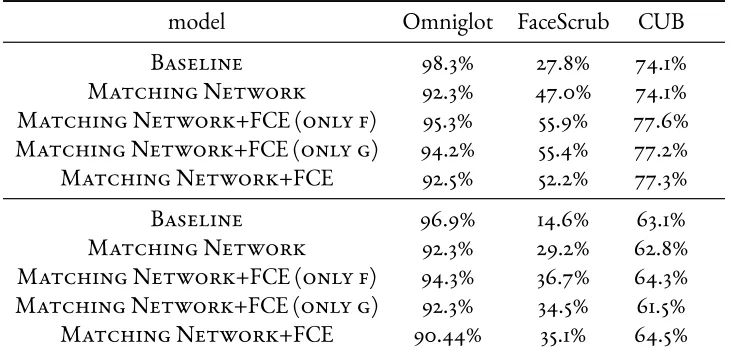
Table 4.2: Test accuracies for different models on vision tasks withN =5,k = 1(top half) andN =10,k = 1
(bo om half). The difference between Baseline and Matching Networks is the use of low-shot training, which we find to have mixed results. On an easier dataset like Omniglot, we find that the baseline outperforms the specialized training. We find the opposite for FaceScrub. Low-shot training is not applicable to CUB because we used pretrained features. We experiment with the effects of using full-context embeddings (FCE) on onlyf(·), onlyg(·), and on both. We find that using FCE generally improves accuracy, though not necessarily using both types.
trained for 20,15,50,25 epochs respectively for Omniglot, FaceScrub, CUB, and QANTA.
Whenever relevant, we tied the parameters between the embedding functionsf(·)andg(·)so that
the model learned the same embedding space for both inputs rather than two different spaces. We
found that this almost always led to improved performance than leaving the models untied.
4.3 Results
We present the results of our one-shot vision tasks forN =5 andN = 10 in Table 4.2. The results of the five-shot learning experiments are reported in Table 4.3. Language experiment results are
4.3.1 Low-Shot Training and Full-Context Embeddings
We highlight a number of interesting trends from our results of one-shot vision experiments. For all
tasks, we see a predictable trend of decreased accuracy when moving fromN =5 toN=10 because
the task is harder when needing to distinguish between more classes. Among all three tasks, the
Omniglot results are the highest, which is unsurprising given the relative easiness of this task. Our
results are in-line with other papers applying one-shot learning methods to this dataset, e.g.Koch
(2015) andVinyals et al.(2016). The CUB results are surprisingly high given the relative difficulty
of the dataset, largely because the features used are from a highly expressive and thoroughly trained
model. Finally, perhaps unsurprisingly, the FaceScrub results are the lowest of the three tasks. They
are significantly below that of state-of-the-art results, but we reiterate that the strength of the model
and embedding function used is that they are very general, rather than being crafted for the
particu-lar task of facial recognition.
Unlike what was found byVinyals et al.(2016), we find that our simple baseline is able to
essen-tially solve these two Omniglot tasks, outperforming any of our specialized low-shot learning
mod-els. On the other hand, low-shot training does seem to lead to significant gains on FaceScrub. For
the CUB dataset, because we are using pretrained features and we evaluate the baseline and
match-ing networks in the same way, there is predictably little difference in test accuracy. The discrepancy
between the benefits of low-shot training is perhaps due to the properties of the dataset. There is
less variation between different classes in Omniglot; most images are a black character in the middle
of a white background. Thus, the patterns that the convolutional filters learn to detect likely carry
over well to new classes. On the other hand, there is significant variation within and between classes
for FaceScrub: faces can be rotated, under different lighting conditions, wearing accessories, etc.
Thus, training to identify people belonging to one set of classes may not carry over as well to
model Omniglot FaceScrub CUB
Baseline 99.62% 31.2% 87.6%
Matching Network 96.9% 56.7% 88.0%
[image:34.612.117.496.97.180.2]Matching Network+prototypes 98.2% 60.0% 90.5% Matching Network+FCE+prototypes 94.9% 62.3% 85.7%
Table 4.3: Test accuracies for experiments with different models on vision tasks withN =5,k=5. We find again that matching networks and all variants are outperformed by our baseline on Omniglot. For all datasets, we see an accuracy improvements over the base matching networks when using prototypes. But when we combine prototypes with full-context embeddings, we get mixed results.
matching networks noticeably underperform the baseline on Omniglot.
We see some modest to significant accuracy gains in using either full-context embeddings forf(·)
org(·)for almost all our experiments. Across all datasets, we see a performance bump when using
onlyf(·)context embeddings relative to the basic matching networks. When we only use full-context embeddings forg(·), we usually see a performance increase, though smaller than that off(·),
and we occasionally get no increase or a small decrease. When we combine the full-context
embed-dings for bothf(·)andg(·), we see either no change or a performance decrease as compared to the
basic matching networks. This decrease is perhaps due to the difficulty in training both types of
full-context embeddings simultaneously. Due to stability issues, we found it necessary to train with a
lower learning rate. Overall, these trends suggest that there is a benefit in giving the model
parame-ters to share information between the support set and batch element embeddings, particularly when
the dataset is relatively complex, for example if it had natural images.
4.3.2 Prototypes
We find many of the similar trends in moving to the five-way, five-shot setting. Where comparable,
the models perform better because the task is easier with five examples per new class rather than only
model QANTA (hist.) QANTA (lit.)
Baseline 23.2% 25.7%
Matching Network 47.5% 40.4%
Matching Network+FCE (only f) 42.9% 37.9% Matching Network+FCE (only g) 44.2% 39.1%
[image:35.612.128.484.95.195.2]Matching Network+FCE 42.4% 36.8%
Table 4.4: Test accuracies for different models on language tasks withN =5,k =1. We find that using low-shot training significantly improves upon using standard training methods. Using any type of full context embedding, on the other hand, degrades performance no ceably.
We see a modest accuracy bump in using class prototypes that is consistent across all datasets,
suggesting that the prototypes do better summarize the class than the examples of that class
individ-ually. Results are mixed when combining prototypes with full-context embeddings. For FaceScrub,
using both leads to a performance increase. With Omniglot and CUB we see a large drop in
perfor-mance, perhaps again pointing to the difficulty of training full-context embeddings.
4.3.3 Language Results
For our language experiments, we find that without using low-shot training, we are not able to get
test accuracy much above that of random guessing. In using low-shot training, we saw initial
train-ing and validation accuracy around 20%. By the end of traintrain-ing, traintrain-ing accuracy jumped to > 90%,
while validation hovered around 40%, indicating that our models had both generalized and overfit
the training data. As the only learnable parameters in the basic matching networks are the word
em-beddings, it seems that allowing fine-tuning of the word embeddings to the task is crucial in getting
good performance. We explore these tuned embeddings in Chapter 5. We also find that using any
5
Analysis
We now explore various methods to better understand what each model learned and
the differences between model architectures.
Visualizations are a powerful qualitative tool in gaining insight to what a model has learned. We
can visualize each model’s weights to inspect for interpretable patterns or lack thereof, and to some
5.1 Visualizing Convolutional Filters
Developing techniques for visualizing what a CNN learns is an active body of research in itself. A
simple visualization method is visualizing the early convolutional layers’ weights. We do so by
rescal-ing the filter weights to normal pixel intensity ranges and display the weights as a images. We show
our visualizations from our baseline and basic matching network models trained on Omniglot and
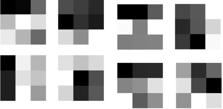
Facescrub in Figures 5.1, 5.2, 5.3, and 5.4. We display a greater subset of filters in Appendix B.
For the Omniglot filters, darker squares correspond to higher weight values. Based off the
pat-terns of darker squares, it appears that both networks learn to pick up on edges and corners. This
matches common intuition that the early convolutional layers should act as low-level feature
extrac-tors, for example by picking up on edges, corners, or color patterns. The similarity of the two sets of
filters is unsurprising given that both performed well on the Omniglot task.
For FaceScrub, both networks’ filters seem to primarily pick up on patches of different colors, for
example in the blue patches or skin-tone patches. This again seems to match our intuition of early
filters as low-level feature detectors. A few filters also seem to activate on color gradients, hinting
at some edge detection capabilities. A substantial portion of the filters are largely grayish, which
possibly indicate dead filters or insufficient training. Between the two networks, anecdotally the
matching network filters seem more intense in color and less grayish, which perhaps begins to get at
performance differences between the two. However, by and large, the two sets of filters seem similar.
More filters are shown in Appendix B.
5.2 Visualizing Word Embeddings
For the language tasks, we can visualize the word embeddings for the model before and after
fine-tuning for low-shot learning. Visualizing these embeddings is particularly insightful because the
Figure 5.1:Visualiza on of a subset of the first convolu-on layer weights (3x3) in the baseline Omniglot model. Darker shaded squares indicate higher weight values. The model learns to pick up on edges and corners, match-ing our intui on that they should detect low-level image features.
Figure 5.2:Visualiza on of first convolu on layer weights (3x3) in the basic matching network model applied to Omniglot. Similar to the baseline model, the matching network filters pick up on edges and corners.
Figure 5.3:Visualiza on of a subset of the first convolu-on layer weights (7x7) in the baseline Facescrub model. The filters seem to pick up on different colors, another low-level feature. The models seem to learn similar first
[image:38.612.110.506.394.593.2]account for the nearly 20% difference in performance.
For each dataset, we take the 2000 most common words and use the t-SNE algorithm (Maaten &
Hinton,2008) to project them to two dimensions, which we can then use to plot the embeddings.
The t-SNE algorithm is a stochastic algorithm that focuses on preserving local structure of the
high-dimensional vector space in projecting to a lower-high-dimensional space. However, the t-SNE algorithm
is not ideal for comparing across models because of its stochasticity. We present a subset of the
re-sulting plots in Figures 5.5, 5.6, 5.7, and 5.8, and present the full t-SNE plots in Appendix B
The original word vectors for both subjects were trained using a word2vec model (Mikolov
et al.,2013), which has been found to produce word vectors that capture semantic meaning. We
can see this effect in Figures 5.5 and 5.7. The t-SNE algorithm tends to preserve clusters in the
high-dimensional space, and we can see in our plots that the embeddings for historical leaders and authors
are clumped together, indicating that the original word vectors carried significant semantic
infor-mation about each word. However, using the untuned word embeddings get train and test accuracy
only slightly above random chance (~20%). When tuned for low-shot learning, train accuracy shoots
up to >90% while test accuracy jumps to approximately 40%. These scores indicate that the model is
overfitting the parameters to the training data, but there is still some generalization happening,
per-haps due to similarity of question formats and common references in train and test data. In training
we lose the semantic coherence of the word embeddings, as shown by the dispersion of the
previ-ously clumped entities amongst nonentity words in Figures 5.6 and 5.8. There is no obvious
inter-pretation to the new embedding space that the model learns, perhaps indicating that there are other
factors than semantic meaning that are important in solving this one-shot task, such as sentence
Figure 5.5:Subset of t-SNE plot of word embeddings for QANTA history ques ons before fine-tuning for low-shot learning. Featured are a clump of historical figures, including Richard_Nixon and Abraham_Lincoln, which matches our intui on that the word vectors of words with similar seman c meaning are close in the embedding space.
Figure 5.6:Subset of t-SNE plot of word embeddings for QANTA history ques ons a er fine-tuning for low-shot learning. The clump of historical figures has become dispersed, as shown by the Richard_Nixon and Abra-ham_Lincoln now spread amongst non-en ty tokens. As a whole the word embeddings do not cluster by seman c meaning clearly as before.
Figure 5.7:Subset of t-SNE plot of word embeddings for QANTA literature ques ons before fine-tuning for low-shot learning. Featured are a clump of authors, including Nikolai_Gogol and Thomas_Mann, demonstra ng that the word vectors for this dataset similarly cluster word vectors
[image:40.612.105.510.406.562.2]6
Conclusion
In this work we performed a close study of matching networks, a recently proposed
neural network and nonparametric hybrid designed for low-shot learning, by evaluating it against a
strong baseline on a diverse set of tasks.
We saw that matching networks indeed are general enough to be applied to a broad range of tasks
datasets, existing models are already able to perform low-shot learning by virtue of the
represen-tations they learn. For more complex datasets, however, specialized low-shot learning methods do
yield significant performance gains over non-specialized approaches. Visualizing what a matching
network learned as compared to a baseline or pretrained weights reveals that when both do well, the
models learn similar feature representations. On the other hand, when matching networks
outper-form, they do seem to learn different, albeit less interpretable, representations, suggesting that there
is still progress to be made in representation learning for text.
There are a number of interesting directions to continue exploring. First, from a modeling
per-spective, we could implement sensible architectures to use the input embeddings to modify the
sup-port set embeddings, akin to the memory update in memory networks. Relatedly, it seems
worth-while to explore simpler architectures to implement full-context embeddings to see if the gains are
from giving the model the parameters to share information or from the specific architecture we
used.
Second, the runtime of matching networks scales linearly in the size of the support set, or at least
the number of classes if we use class prototypes. For some applications, however, this may still be
infeasible because of a very high number of classes, for example if we wanted to perform one-shot
learning over all of the Omniglot classes. There has been a number of recent papers exploring
hierar-chical approaches to prediction over a large number of classes that would be interesting to combine
with matching networks.
Third, for some of our datasets, our model still had access to tens of thousands of examples
throughout training. It would be interesting to see how well the model holds up when it only sees a
few thousand or even fewer examples during training.
Additionally, a benefit of having such a general model is that it can be applied to nearly any
prob-lem. There many more applications of matching networks worth exploring, such as to medical
In sum, there remains a significant amount of work to be done before we have general
architec-tures capable of true low-shot learning. Future progress on this task will likely require building
bet-ter representations for specific problem domains as well as building betbet-ter general low-shot learning
frameworks. We hope that our work inspires the development of new model architectures, datasets,
A
Common Neural Architectures
A.1 Convolutional Neural Networks
Convolutional neural networks (CNNs) were largely born out of a need to create models that could
process images with relatively few parameters. Using a fully connected layer to process an image,
meaning multiplying each pixel intensity (3 intensities per pixel for a standard RGB image) of the
~50,000 weights for a single layer. Over multiple layers and larger images, this architecture would
quickly become unwieldy. CNNs get around this issue by using a small weight matrix that is
ap-plied as a dot product to each possible patch in the image, so that the weights are shared across all
image patches. Intuitively, we can think of this weight matrix as detecting or filtering for a specific
pattern within the image patch it is applied to, and thus we typically refer to the matrix as a filter
or kernel. By “sliding” the filter across the image to apply it to all image patches, we are convolving
it with the image, the eponymous convolution. Within a convolutional layer, we do not need to
restrict ourselves to a single filter, but instead we can use multiple convolutional filters so that the
model can learn to detect multiple patterns at each layer while still using far less parameters than
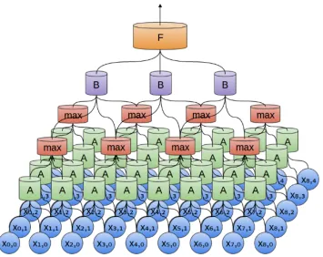
fully connected layers. Figure A.1 depicts the process of applying a convolution over an image.
While it is possible to stack convolutional layers (i.e. apply a convolution to the output of a
con-volution), in practice it is more common to use pooling layers between convolutional layers, which
like convolutional layers perform some operation over a small patch and are repeated over the
en-tire input. Unlike convolutional layers, however, pooling operations typically do not involve extra
parameters. The most common pooling operation is max-pooling, which takes the max value over
some image patch, but other common operations include average pooling and min pooling.
Pool-ing is commonly used to reduce the size of its input and have the added benefit of makPool-ing the CNN
somewhat robust to small affine change or rotations in an image. For both convolution and pooling
layers, we can not only vary the size of the kernel, but we can also vary the frequency with which we
apply the filters. The pooling operation is also depicted in Figure A.1.
The two other types of layers that we use in our CNNs are nonlinear layers and batch
normal-ization layers. Nonlinear layers are any nonlinear function applied elementwise to its input, and for
neural networks it is common to use the rectified linear unit (ReLU;f(x) = max(0,x)), sigmoid
(f(x) = 1+e1−x), or tanh (f(x) = e x−e−x
ex+e−x). Batch normalization was introduced byIoffe & Szegedy
but on a high level batch normalization works by normalizing (subtracting the mean and dividing
by the standard deviation) over a batch and then applying an affine transformation that is learned
throughout training. This procedure stabilizes training by making the inputs to the following layer
follow the same distribution throughout training rather than shifting.
We compose our CNNs by arranging convolution modules, each of which consists of a
convolu-tion, followed by batch normalizaconvolu-tion, a ReLU nonlinearity, and a max pooling layer. We pad each
of our convolution layers such that the convolution preserves the input shape, and we do not pad
the max-pooling layers but do use stride 2, so that the max-pooling layer halves each input
dimen-sion.
A.2 Recurrent Neural Networks
Recurrent neural networks (RNN) are a class of neural networks that are designed to give the
mod-els some internal capacity for “memory” to remember its previous inputs. In broad terms, this
“memory” is achieved by adding a hidden state vectorhtto the model that encodes the sequence
of previous inputsx1,x2, . . .xt−1that the model has seen. With each input, an RNN updates its
hid-den state using the current hidhid-den state and input:ht =R(ht−1,xt)whereh0is initialized to some
value, most commonly the zero vector. Recurrent neural networks, then, are so named because we
must recursively apply the functionR(·)in order to get an output.
We provide a more specific formal description of the variant of RNN we use in our experiments,
known as the long short-term memory (LSTM;Hochreiter & Schmidhuber(1997)). We closely
followGreff et al.(2016) in defining the LSTM. The notation introduced here is independent of the
notation used elsewhere in this work.
An LSTM is designed to better capture long-range dependencies within a sequence via a series
inputs, as well as two types of internal state: the hidden stateht ∈ Rd′and the cell statect ∈ Rd′.
At each time step, new values for the gates are computed from the current input, hidden state, and
cell state. The inputxt ∈ Rdis combined with the previous hidden stateht−1to producezt ∈Rd
′
.
The input gateitcontrols how much of this combinationztis passed forward to compute the new
cell state. The forget gateftcontrols how much from the previous cell statect−1is carried over. The
input and forget gates are combined with their respective information flows to compute the new
cell statect. Finally, the output gateotcontrols how much of this new cell state is passed forward to
compute the next hidden stateht. This process is depicted in Figure A.2.
More technically, gates and states are computed using the following update rules:
zt=σ(Wzxt+Rzht−1+bz) (A.1)
it=σ(Wixt+Riht−1+pi⊙ct−1+bi) (A.2)
ft=σ(Wfxt+Rfht−1+pf⊙ct−1+bf) (A.3)
ct=ft⊙ct−1+it⊙zt (A.4)
ot=σ(Woxt+Roht−1+po⊙ct−1+bo) (A.5)
ht=ot⊙tanh(ct) (A.6)
also applied pointwise to its argument. Usingσsquashes the gate values to be in[0,1], where 0
cor-responds to passing no information through and 1 corcor-responds to passing all information through.
Thep∗vectors are known as peephole connections because they allow the model to “peep” at the
current cell state in computing the gate next values. The matricesW∗ ∈ Rd×d′andR∗ ∈ Rd′×d′, biasesb∗ ∈Rd′, and peepholesp∗ ∈Rd′are learnable parameters that are trained used
backpropa-gation.
For a sequencex1,x2, . . . ,xTwe can apply an LSTM to the elements of the sequence in order
and also apply an LSTM to the sequence in reverse, and then combine the two resulting sequences
of hidden states in some way, e.g. vector addition or concatenation. Using two LSTMs in this way
produces a bidirectional LSTM.
In applying LSTMs to matching networks, we use LSTMs for our full-context embeddings.
Specifically, we use a bidirectional LSTM to embed the support set conditioned on each other
and we use an LSTM with attention over the support set at each time step to embed the batch of
test inputs as specified in the model. We also briefly explored using an LSTM over the words of
the QANTA questions but found that it did not perform well due to issues with uneven sentence
Figure A.1:A diagram of a CNN. The blue circles at the bo om represent the input. Each of theAcylinders is the same convolu onal filter that computes a dot product between its weights and all possible 2x2 patches in the input, as indicated by the blue circles each is connected to. No ce that each circle in the input is operated on by mul ple
Figure A.2:A diagram of the computa on graph for a single me step update in an LSTM. Arrows represent values being passed as func on inputs,⊗represents elementwise mul plica on, the node immediately a er the cell is a
tanh(). The inputxt(le ) is combined with the hidden stateht−1to computezt. The input, output, and forget gates
are computed using cell state, hidden state, and input. The input gate is combined elementwise withztand the forget
gate is combined elementwise with the previous cell statect−1. Those two products are used to compute the current
cell statect, which is then mul plied elementwise with the output gate to compute the new hidden stateht. Figure
Additional Visualizations
[image:52.612.124.486.241.537.2]B.1 Convolutional Filters
B.2 Word Embeddings
[image:56.612.151.477.199.531.2]Note: these figures won’t be readable in print, but can be zoomed in on in electronic formats.
References
Fei-Fei, L., Fergus, R., & Perona, P. (2006). One-shot learning of object categories. IEEE transac-tions on pattern analys and machine intelligence, 28(4), 594–611.
Graves, A., Wayne, G., & Danihelka, I. (2014). Neural turing machines. arXiv preprint arXiv:1410.5401.
Greff, K., Srivastava, R. K., Koutník, J., Steunebrink, B. R., & Schmidhuber, J. (2016). Lstm: A search space odyssey.IEEE transactions on neural networks and learning systems.
Hill, F., Bordes, A., Chopra, S., & Weston, J. (2015). The goldilocks principle: Reading children’s books with explicit memory representations.arXiv preprint arXiv:1511.02301.
Hochreiter, S. & Schmidhuber, J. (1997). Long short-term memory. Neural computation, 9(8), 1735–1780.
Huang, G. B., Ramesh, M., Berg, T., & Learned-Miller, E. (2007). Labeled fac in the wild: A database for studying face recognition in unconstrained environments. Technical report, Technical Report 07-49, University of Massachusetts, Amherst.
Ioffe, S. & Szegedy, C. (2015). Batch normalization: Accelerating deep network training by reduc-ing internal covariate shift.arXiv preprint arXiv:1502.03167.
Iyyer, M., Boyd-Graber, J. L., Claudino, L. M. B., Socher, R., & Daumé III, H. (2014). A neural network for factoid question answering over paragraphs. InEMNLP(pp. 633–644).
Koch, G. (2015). Siamese neural networks for one-shot image recognition. PhD thesis, University of Toronto.
Lake, B. M., Salakhutdinov, R., & Tenenbaum, J. B. (2015). Human-level concept learning through probabilistic program induction.Science, 350(6266), 1332–1338.