Global Waste
Management Outlook
i
t
e
d
n
a
t
i
o
n
s
e
n
v
i
r
o
n
m
e
n
t
P
r
o
g
r
a
m
m
e
United Nations Environment Programme P.O. Box 30552 Nairobi, 00100 Kenya
Tel: (254 20) 7621234 Fax: (254 20) 7623927 E-mail: [email protected]
web: www.unep.org
www.unep.org
U
n
i
t
e
d
n
a
t
i
o
n
s
e
n
v
i
r
o
n
m
e
n
t
P
r
o
g
r
a
m
Copyright © United Nations Environment Programme, 2015
This publication may be reproduced in whole or in part and in any form for educational or non-profit purposes without special permission from the copyright holder, provided acknowledgement of the source is made. UNEP would appreciate receiving a copy of any publication that uses this publication as a source.
No use of this publication may be made for resale or for any other commercial purpose whatsoever without prior permission in writing from the United Nations Environment Programme.
Disclaimer
The designations employed and the presentation of the material in this publication do not imply the expression of any opinion whatsoever on the part of the United Nations Environment Programme concerning the legal status of any country, territory, city or area or of its authorities, or concerning delimitation of its frontiers or boundaries. Moreover, the views expressed do not necessarily represent the decision or the stated policy of the United Nations Environment Programme, nor does citing of trade names or commercial processes constitute endorsement.
Mention of a commercial company or product in this publication does not imply endorsement by the United Nations Environment Programme
ISBN: 978-92-807-3479-9 DTI /1957/JA
UNEP promotes
environmentally sound
practices globally and in
its own activities. This publication
Acknowledgements
This publication is dedicated to the memory of Matthew Gubb, who passed away during the development of the Global Waste Mangement Outlook (GWMO). As Director of UNEP-IETC, Matthew was heavily involved in the initial planning of the GWMO, but he was sadly unable to participate in its preparation.
Core Team Editor-in-Chief
David C. Wilson (Independent waste and resource management consultant and Visiting Professor in Waste Management at Imperial College London, UK).
Authors
David C. Wilson, Ljiljana Rodic (Senior Researcher, Wageningen University and Research Centre, Wageningen, The Netherlands), Prasad Modak (Executive President of Environmental Management Centre (EMC) LLP, India), Reka Soos (Director of Resources and Waste Advisory Group and Managing Director of Green Partners, Romania), Ainhoa Carpintero Rogero (Associate Programme Officer, UNEP-IETC), Costas Velis (Lecturer in Resource Efficiency Systems, School of Civil Engineering, University of Leeds, UK), Mona Iyer (Associate Professor at Faculty of Planning, CEPT University, Ahmedabad, India), and Otto Simonett (Director and co-founder of Zoï Environment Network, Switzerland).
Authorship of the six chapters and specific contributions Chapter 1: Waste Management as a Political Priority
David C. Wilson and Ainhoa Carpintero Rogero
Chapter 2: Background, Definitions, Concepts and Indicators David C. Wilson and Ainhoa Carpintero Rogero
Chapter 3: Waste Management: Global Status Prasad Modak, David C. Wilson and Costas Velis Chapter 4: Waste Governance
Ljiljana Rodic
Chapter 5: Waste Management Financing Reka Soos, David C. Wilson and Otto Simonett
Chapter 6: Global Waste Management – The Way Forward David C. Wilson
Case Studies
Mona Iyer and Ainhoa Carpintero Rogero Academic advisors
Costas Velis, Ljiljana Rodic Communications advisor Otto Simonett
Project Coordinator Ainhoa Carpintero Rogero
Special support from: Kata Tisza (Technical Manager, ISWA) and Rachael Williams Gaul (Technical Manager, ISWA – until February 2015).
Supervision
Surendra Shrestha (Director, UNEP-IETC), Surya Chandak (Senior Programme Officer, UNEP-IETC), David Newman (President, ISWA) and Hermann Koller (Managing Director, ISWA).
Steering Committee
Gary Crawford (Vice President – Sustainable Development Technical, Scientific and Sustainable Development Department, Veolia Environmental Services, France), Johannes Frommann (Senior Advisor, Deutsche Gesellschaft fuer Internationale Zusammenarbeit (GIZ), Germany), Christian Holzer (Director General Federal Ministry of Agriculture, Forestry, Environment and Water Management, Austria), Hermann Koller (Managing Director, ISWA, Austria), Raquel Lejtreger (Vice Minister, Subsecretary, Ministry of Housing, Spatial Planning and Environment, Uruguay) Stanley Motsamai Damane (Director, National Environment Secretariat, Ministry of Tourism, Environment and Culture, Lesotho), Nadzri bin Yahaya (Director General, National Solid Waste Management Department, Ministry of Housing and Local Government, Malaysia), Carlos RV Silva Filho (CEO ABRELPE, Brazil), Surendra Shrestha (Director UNEP-IETC, Japan).
Peer reviewers and contributors
UNEP peer reviewers and contributors
Meriem Ait Ali Slimane, Cristina Battaglino, Matthew Billot, Garrette Clark, Ludgarde Coppens, Christopher Corbin, Charles Davies, Heidelore Fiedler, Carla Friedrich, Mijke Hertoghs, Arab Hoballah, Shunichi Honda, Matthias Kern, Birguy Lamizana, Mushtaq Memon, Llorenç Milà i Canals, Desiree Montecillo Narvaez, Jordi Pon, Pierre Quiblier, Heidi Savelli, Ibrahim Shafii, Elisa Tonda, Mick Wilson, Kaveh Zahedi.
Thanks to our UNEP colleagues, in particular to: Fuaad Alkizim, Utako Aoike, Junko Fujioka, Azumi Nishikawa, Solange Montillaud-Joyel, Mayumi Morita, Moira O’Brien-Malone, John Peter Oosterhoff, Michiko Ota, Sheeren Zorba.
Thanks to ISWA Members/colleagues, in particular to: Jos Artois (Indaver, Belgium), Josef Barth (Informa, Germany), Gunilla Carlsson (Sysav, Sweden), Adam Read (Ricardo-AEA), Marco Ricci-Jürgensen (CIC Italian Composting and Biogas Consortium, Italy) and the ISWA General Secretariat team.
International Solid Waste Association General Secretariat
Auerspergstrasse 15/41, 1080 Vienna, Austria Tel: +43 1 2536 001 Fax: +43 1 253 600199 E-mail: [email protected] Web: www.iswa.org
Editor: Tara Cannon
WASTE
MANAGEMENT:
GLOBAL
STATUS
3
CHAPTER
Chapter 3 provides a context or setting to the GWMO by presenting data as an evidence
base regarding waste generation and its management across the world.
The Chapter starts by looking at the relative quantities of different types of wastes from
various sources (Section 3.2). The focus then turns to municipal solid waste (MSW) where
data on quantities and composition as well as past trends and future projections are presented
(Section 3.3). Section 3.4 overviews the status of MSW management across income groups
and regions. It focuses first on the protection of public health by ensuring that all wastes are
collected, and then on environmental protection by phasing out uncontrolled disposal and
open burning of waste.
The later sections focus on resource recovery (Section 3.5), looking at collection for recycling,
the importance of source segregation, and available technologies for resource recovery. This
is followed by an examination of the global industry in secondary materials (Section 3.6).
3.1
SUMMARY OF THE CHAPTER – KEY MESSAGES ON THE GLOBAL STATUS OF
WASTE MANAGEMENT
1•
A best ‘order of magnitude’ estimate of the total global arisings of municipal solid waste (MSW) is around 2 billion tonnes per annum. A broad grouping of ‘urban’ wastes, including MSW, commercial and industrial (C&I) waste, and construction and demolition waste (C&D), is estimated at around 7 to 10 billion tonnes per annum.•
Although generation rates vary widely within and between countries, MSW generation per capita is strongly correlated with national income. In high-income countries, MSW generation rates are now beginning to stabilize, or even show a slight decrease, which may indicate the beginning of waste growth ‘decoupling’ from economic growth. However as economies continue to grow rapidly in low- and middle-income countries, one can expect per capita waste generation to increase steadily.•
Waste generation is growing rapidly in all but the high-income regions of the world, as populations rise, migration to cities continues, and economies develop. In 2010, the traditional high-income countries accounted for around half of all waste generation. That is forecast to change quickly, with Asia overtaking these countries in terms of overall MSW generation by around 2030 and Africa potentially overtaking both later in the century.•
Organic fractions comprise a greater percentage of the MSW arisings in low-income countries (where organic waste is typically 50 to 70% of all MSW) than in high-income countries (where organics account for typically 20 to 40%). The percentage of paper appears to be proportional to income levels (23% of MSW in high-income, 19% to 11% in middle-income and 7% in low-income countries). Plastic levels generally appear high across the board (8% to 12%), not showing as much dependence on income level as other waste types. ‘Dry recyclable’ materials (metals, glass and textiles) range from 12% of MSW in high-income to 12% and 9% in middle-income and then 6% in low-income countries. Household hazardous waste (HHW) is estimated to make up less than 1% of all MSW across all income ranges, but its presence makes certain management options much more difficult.•
Extending MSW collection to 100% of the urban population is a public health priority. Evidence suggests that significant progress has been made in many middle-income countries over the past few years, particularly those with gross national income (GNI) per capita above USD 2500 per year. At the same time, median collection coverage is still around 50% in low-income countries and figures are much lower in some countries. It also drops sharply in the more rural areas of many countries. It is estimated that at least 2 billion people worldwide still lack access to solid waste collection.•
Eliminating uncontrolled disposal is a priority for protecting the environment. Evidence suggests considerable progress has been made. However, the 100% and 95% controlled disposal rates in high- and upper-middle income countries respectively are in stark contrast with rates that are often well below 50% in low-income countries, and 0% controlled disposal is still relatively common in rural areas in many countries. In lower-income countries, waste disposal is often in the form of uncontrolled dumpsites with open burning. It is estimated that at least 3 billion people worldwide still lack access to controlled waste disposal facilities.•
Recycling may provide a source of income, help conserve scarce resources and reduce the quantities of waste requiring disposal. However the success of recycling depends critically on materials being kept separate and clean and being found in sufficiently high concentrations. Recycling rates in high-income countries have progressively increased over the last 30 years, driven largely by legislative and economic instruments. In lower-income countries, the informal sector is often achieving recycling rates of 20 to 30% for MSW.•
The secondary materials industry operates globally, with active international ‘commodity’ markets for ferrous and non-ferrous metals, paper, plastics and textiles. Most secondary materials come from industry and most are utilized inside national boundaries, but a sharp increase in the availability of materials from MSW recycling since the 1990s, together with the relocation of much of the world’s manufacturing industry to Asia in general and to the People’s Republic of China (PRC) in particular, has led to an increasingly transboundary and even global market. The PRC accounts for 60% by weight of global imports ofaluminium scrap, 70% of recovered paper and 56% of waste plastics. Other Asian countries are also major importers, with Turkey the recipient of 30% of the total world trade in steel scrap.2
•
Resource recovery from waste includes processes both for the recovery and recycling of the organic fraction and for energy recovery. Global activity in new waste processing facilities is high. Over the past two years, waste processing investment projects worth more than 300 billion USD have been active, of which 85 billion USD was directed to MSW processing (although not all of these projects will be built). Most of this investment activity is in the high-income countries, including energy from waste projects utilizing biomass and so on.•
Some waste streams require particular focus. Topic sheets are provided in the GWMO for large-volume C&D waste; for high-risk hazardous waste and e-waste; for plastic waste and for its associated problem of marine litter, which is receiving global attention; for waste from disasters; and for food waste, the scale of which is huge when considered alongside food scarcity and global starvation.•
Mining and quarrying and agriculture and forestry residues and wastes are generally managed close to source, with most agriculture and forestry wastes either being returned to the soil as soil improvers and nutrients or used as biomass fuel. These large volume streams are thus generally outside of national waste control regimes and data are not reported. A very rough, ‘order of magnitude’ estimate is that each of these major sectors generates 10 to 20 billion tonnes per annum of residue and waste. Mine tailings merit further attention as waste due to their potential for health and environmental impacts.•
The definitions of waste categories vary widely; waste quantities are often not measured; national reporting systems are often weak. As a result, it is not surprising that international data on MSW generation, composition and management lacks adequate breadth and depth and is weak and unreliable. The international data situation is still worse for other waste types. Use is made here of recent work that developed indicators to benchmark the performance of a city’s MSW management system on a consistent basis. It is recommended that waste and resource management data are actively included within wider international action as part of the data revolution to improve data for sustainable development, that a globally recognized and internationally agreed methodology be developed for collecting and reporting waste data at the local (municipal) and national levels, and that the available performance indicators be subjected to widespread testing, with the results used to inform further work to develop standardized indicators.2 Excluding intra-EU trade.
Compost
© Ainhoa Carpintero
Textile waste
3.2
OVERVIEW OF GLOBAL WASTE GENERATION
[image:9.595.178.449.290.438.2]Providing a global overview of total waste generation would appear to be a fundamental element of the GWMO, but in reality it is almost impossible to do so with sufficient accuracy.3 Where data exist, they generally refer to MSW,4 hence that is the focus for most of this chapter. A wider compilation of data on waste from different points in the material and product life cycle exists mainly in higher-income countries, especially in OECD countries. Therefore these data have been used as a ‘proxy’, to show the relative quantities of waste from different sources.
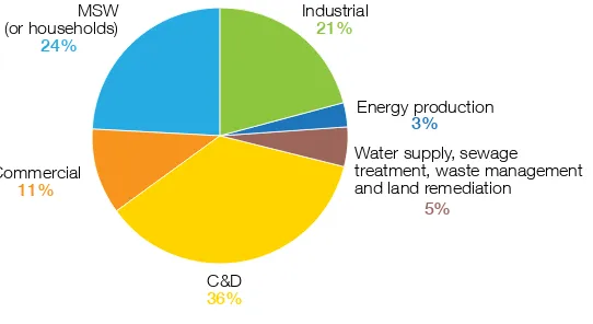
Figure 3.1 suggests that the three major waste streams of construction and demolition (C&D), commercial and
industrial (C&I – appearing as two segments in Figure 3.1) and municipal solid waste (MSW) predominate. In the higher-income OECD countries from which these data are taken, MSW is generally managed by municipalities and C&I and C&D waste by the waste generators themselves through the waste industry (through business to business [B2B] arrangements).5 However, even in these cases there is overlap between the definitions and considerable variation between countries. The distinctions between these three major waste types are even more ‘fuzzy’ in developing country cities.6
Figure 3.1 Relative quantities of waste from different sources in the material and product life cycle
MSW (or households)
24%
Industrial
21%
Energy production 3%
Water supply, sewage treatment, waste management and land remediation
C&D 36% Commercial
11%
5%
Notes: Data is for the OECD countries as a proxy, due to limitations on availability of data from the rest of the world. All data exclude agricultural and forestry and mining and quarrying wastes. Where there are significant gaps in the OECD database for a particular waste arising in a specific country, other sources have been used (using the EMC Master database [2014, n.p.] compiled for the GWMO), or an estimate has been made. Estimate of waste from a broad range of municipal, commercial and industrial sources (total waste quantity generated in the OECD countries, including construction and demolition (C&D) but excluding agricultural and forestry and mining and quarrying): 3.8 billion tonnes per annum.
Figure 3.1 distinguishes two further types of waste, which are reported separately in the OECD database. Wastes
arising from water supply, sewage treatment, waste management and land remediation represent around 5% of the total, while waste from power generation represents around 3%. These sources are interesting, as they represent the best measure available of those residues which have been removed from emissions to air and water, and concentrated as ‘solid waste’.7
In principle, it is possible to attempt to extrapolate from the OECD data in Figure 3.1 to estimate total worldwide waste arisings. Such extrapolation is facilitated by the availability of waste data for some non-OECD countries, in particular Russia and the PRC.8 Extrapolating from the EMC database prepared for the GWMO to estimate 2010 worldwide MSW arisings results in an estimate of around 2 billion tonnes per annum, which is roughly twice the MSW figure for the OECD.
For the other waste streams, extrapolation is even more challenging. Based on the available information, the best ‘order of magnitude’ estimate of total arisings worldwide for the broad grouping of ‘urban’ wastes (municipal, commercial and industrial wastes, including C&D waste) comparable to the data indicated for the OECD in Figure 3.1 is in the range of 7 to 10 billion tonnes per annum. However, more reliable, measured data are urgently needed: a major recommendation from the GWMO is to ensure that waste and resource
3 See Section 2.5.2 on the quality and availability of waste-related data.
4 See Section 3.3 for an overview of municipal standard waste generation, its composition and its properties. 5 See Chapter 5, in particular Sections 5.3 and 5.5.
management data are actively included within wider international action as part of the data revolution to improve data for sustainable development.
A decision was taken early in the development of the GWMO to focus on the ‘higher risk’ grouping of wastes included in Figure 3.1. The two major sectors ‘Agricultural and Forestry’ and ‘Mining and Quarrying’ had been set aside, as these sectors’ residues and wastes are generally managed close to source, with most agricultural and forestry residues either being returned to the soil as nutrients or used as biomass fuel; are often outside of national waste control regimes; and data for them are generally not reported.9 The quantities are potentially very large, as these wastes include crop residues, animal manure and wood residues from agriculture and forestry as well as rock, over-burden and processing residues from mining and quarrying. Based on data from the few countries which collect and report them, and on estimates based on production data and assumptions concerning residues per unit of production, it is possible to make rough, ‘order of magnitude’ estimations of total worldwide arisings of residues and wastes, which are in the range of 10 to 20 billion tonnes per annum for each of the two sectors. The main component of interest in the GWMO, due to its potential impacts on public health and the environment, is mine tailings, on which a specific follow-up study is recommended.
3.3
OVERVIEW OF MSW GENERATION
3.3.1 MSW generation
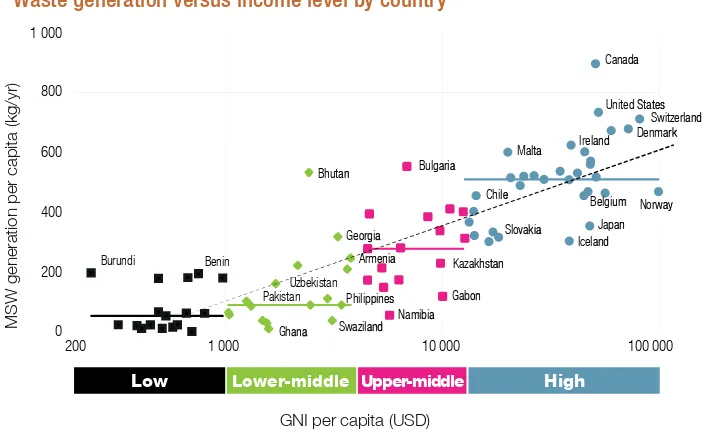
[image:10.595.121.473.428.645.2]MSW generation rates vary widely within and between countries. The generation rates depend on income levels, socio-cultural patterns and climatic factors. Figure 3.2 shows the relationship between waste per capita10 and income levels per capita for 82 countries. Despite the ‘scatterplot’, there is a strong positive correlation, with the median generation rates in high-income countries being about six-fold greater than in low-income countries. There is also considerable variation within countries. For example, Brazil’s national database shows state waste generation per capita in 2012 ranging from a low of 310 kg per capita per annum to a high of 590 kg per capita per annum.11
Figure 3.2 Waste generation versus income level by country
0 200 400 600 800 1 000
200 1 000 10 000 100 000
Low Lower-middle Upper-middle High
MSW generation per capita (kg/yr)
GNI per capita (USD) Burundi Benin
PakistanUzbekistan
Ghana Swaziland Namibia Philippines
Armenia Georgia
Bhutan Bulgaria
Malta
Chile
Slovakia
Kazakhstan
Iceland Japan Belgium Norway Ireland Denmark
Switzerland United States Canada
Gabon
Notes: Based on data from 82 countries using the latest available data within the period 2005-2010. For 12 countries, the latest available data was older than 2005.
Regression: y = 109.67ln(x) – 651.45, R² = 0.72
Data sources: EMC’s Master Country Database (n.p., 2014) using primarily data from the EU, OECD and World Bank; Lawless (2014), Waste Atlas: Recycling and resource recovery around the world (Unpublished master’s thesis). University of Leeds, Leeds, UK. Both were prepared for the GWMO (see Annex B, under Waste databases).
9 See Section 2.2.3.
10 It is important to note that data reported for many countries is likely to be MSW collected rather than generated. This not only affects interpretation of the waste generation data but also the data on waste composition.
3.3.2 MSW Composition and Properties
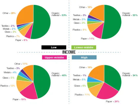
In spite of the high variability and low reliability of source data, a comparison of average compositions relative to the countries’ income level shows some interesting patterns (see Figure 3.3).
•
One major difference is in organic fractions, which are significantly higher in middle- and low-income countries (averaging 46 to 53%) than in high-income countries (averaging 34%). Yet in fact these averages might be understating the differences. One comparative study contrasts an average of 67% across many middle- and low-income cities with 28% for cities in Europe, North America and Australia.12 Also, the nature of the organic waste differs. In middle- and low-income countries, most organic waste is ‘unavoidable’, as it is the organics left over after the preparation of fresh food – organic matter that could not have been eaten. In contrast, in high-income countries there is a great deal of avoidable food waste – that is, food that could have been eaten.13•
The percentage of paper waste appears to be proportional to income levels, rising steadily from 6% in low-income countries, through 11% to 19% in middle-income and 24% in high-income countries. These figures are in line with data on the annual per capita consumption of paper worldwide, which ranges from 240 kg in North America, through 140 kg in Europe, to 40 kg in Asia and 4 kg in Africa. There has long been speculation that per capita consumption of printing and writing paper and newsprint in high-income countries has been falling due to electronic readers. The world average per capita consumption had shrunk by 4% in 2012 compared to the peak recorded in 2007.14•
While plastic levels appear generally high, they perhaps do not show as much dependence on income level as might be expected, with the averages for all income categories having a fairly narrow range of 7 to 12%. However, these averages do hide considerable variation between countries, with much higher values being reported in certain countries. For example, a regional comparative report indicated high levels for both Jordan (about 16%) and Mauritania (about 20%).15•
Levels of other ‘dry recyclable’ materials, which include metals, glass, and textiles, are all relatively low. Taken in aggregate, there is a small but steady increase in this type of waste as incomes rise, from 6% in low-income countries, through 9% and 12% in middle-income to 12% in high-income nations.•
MSW now increasingly contains relatively small amounts of hazardous substances. Often known as household hazardous waste (HHW), typical sources may include mineral oils such as motor oil; asbestos products such as roofing and heating blankets; batteries; waste electrical and electronic equipment (WEEE or e-waste); paints and varnishes; wood preservatives; cleaning agents such as disinfectants; solvents such as nail varnish; pesticides such as rat poison; cosmetics such as hair dyes; and photo lab chemicals such as developer. Statistics are unavailable on the percentage of household hazardous waste in MSW on a global basis. Estimates suggest a percentage of household hazardous waste in MSW of less than 1%, but up to 5% if e-waste is included.16Waste composition affects the physical characteristics of the waste, including density, moisture content and calorific value, which in turn affect waste management and the choice of technology for collection, treatment and the 3Rs. For example, the ash content of MSW in high-income countries has decreased over the last 50 years, while the content of paper, plastics and other packaging materials has increased, significantly reducing the bulk density and increasing the calorific value. Reduced density has increased the need for compaction during collection to achieve higher and more economic vehicle payloads, while increased packaging content and rising calorific values make both recycling and energy from waste (EfW) more attractive. Conversely, the higher levels of organic waste in lower-income countries means that the waste is wetter, denser and has a lower calorific value, so there is less need for compaction during collection and the MSW may not burn without auxiliary or support fuel.
Some plastic wastes, in particular PVC, can result in air emissions of toxins such as dioxins and furans if unmanaged wastes are subjected to open burning, or if the thermal treatment and pollution control at EfW
12 Wilson et al. (2012). Comparative Analysis of SWM in 20 cities. 13 of the 15 ‘Southern’ middle- and low-income countries are within the range 48–81% (average 67%); while the five cities in Europe, North America and Australia (i.e. the four high-income cities plus Varna in Bulgaria) report 24–34% (average 28%). Source listed in Annex A, under Chapter 1, Waste management.
13 See Topic Sheet 11 on Food Waste and Case Study 3 on reducing food waste, both found after Chapter 3.
14 Bureau of International Recycling (2014). Recovered paper market in 2012 (2014 report), listed in Annex A, Chapter 3, Global secondary materials industry. 15 Sweepnet (2014a), listed in Annex A, Chapter 2, Waste data and indicators.
facilities are inadequate. In light of this, it is important to establish a reliable database on waste composition and characteristics and monitor the trends.
Figure 3. 3 Variation in MSW composition grouped by country income levels
Other •19%
Textiles •1%
Metals •5%
Organic material •34%
Paper •24%
Glass •6%
Plastics •11% Other •11%
Textiles •3%
Metals •4% Organic
material •46%
Paper •19%
Glass •5%
Plastics •12%
Other •18%
Textiles •3%
Metals •3%
Organic material •53%
Paper •11%
Glass •3%
Plastics •9% Other •28%
Textiles •2%
Metals •2%
Organic material •53%
Paper •6%
Glass •2%
Plastics •7%
Low Lower-middle
Upper-middle High
INCOME
Notes: Based on data from 97 countries (22 in Africa; 14 Asia-Pacific; 35 Europe; 19 Latin America/Caribbean; 2 North America; 5 West Asia). Dates of the data vary between 1990-2009. “Other” means other inorganic waste.
Source: EMC’s Master Country Database (n.p., 2014) using primarily data from the UN and World Bank and Hoornweg & Bhada-Tata (2012)17
3.3.3 Trends in MSW generation
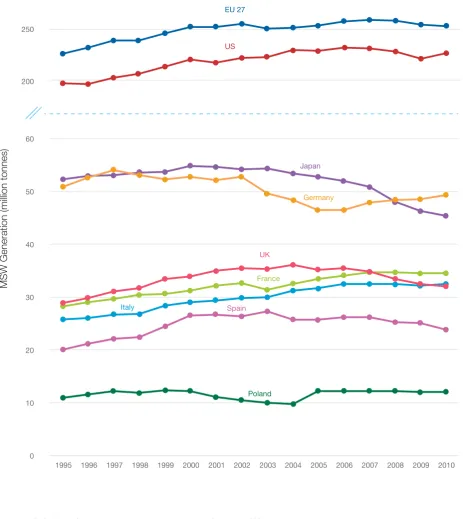
Waste generation per capita has risen markedly over the last 50 years and shows a strong correlation with income level. Figure 3.4 shows data for the last 20 years in some high-income countries. This figure also suggests that MSW generation rates are beginning to stabilize in high-income countries, or even show a slight decrease. This is often cited as evidence for the beginning of waste growth ‘decoupling’ from economic growth, as the trend became apparent before the 2008-09 financial crisis. However, the previous rising trend may resume if economic growth returns to previous levels. Also, a contributing factor may be the shifting of manufacturing industries to emerging economies. This shift would not be such a major factor in MSW generation, but would be expected to have a larger impact on industrial waste quantities.
Figure 3. 4 Trends in MSW generation since 1995 in selected high-income countries
0 10 20 30 40 50 60 200 250 300
1995 1996 1997 1998 1999 2000 2001 2002 2003 2004 2005 2006 2007 2008 2009 2010
France
UK
Japan
US EU 27
Germany
Italy Spain
Poland
MSW Generation (million tonnes)
Data source: EMC’s Master Country Database (n.p., 2014) using data from Eurostat and OECD
The best available data on current total world generation of MSW come from a combination of ‘real’ national statistics, where waste arisings have been systematically measured, recorded and reported; and calculated figures where population data have been combined with estimates for MSW generation per capita. Forward projections of both population and waste per capita data are needed to project these figures into the future and forecast future changes in MSW arisings.
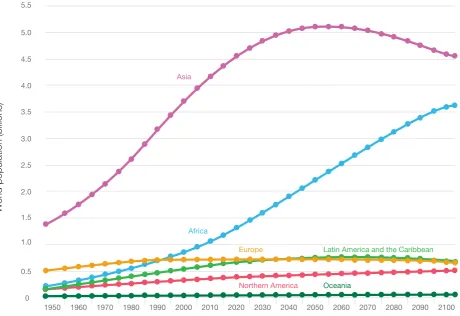
Forecasting population has been a major focus for the world’s statisticians. The UN’s World Population Prospects18 publishes a range of scenarios for future population growth through to 2100, although the scenarios begin to show an increasingly broad range in their forecasts beyond the next 30 years. Figure 3.5 shows estimated and projected world population by region from 1950 to 2100 for the ‘medium variant’. The general
trend is an initial rise, followed by a levelling out and then either a stabilization or a fall. Under this scenario, Asia is forecast to reach its peak population around 2050 while Africa continues to grow through to 2100.
Figure 3. 5 Estimated and projected world population by region
0 0.5 1.0 2.0 2.5
1.5 3.0 3.5 4.0 4.5 5.0 5.5
1950 1960 1970 1980 1990 2000 2010 2020 2030 2040 2050 2060 2070 2080 2090 2100
Asia
Africa
Europe Latin America and the Caribbean
Northern America Oceania
W
orld population (billions)
Notes: Estimates: 1950-2010; Medium variant: 2015-2100 Source: UNDESA, Population Division (2013)19
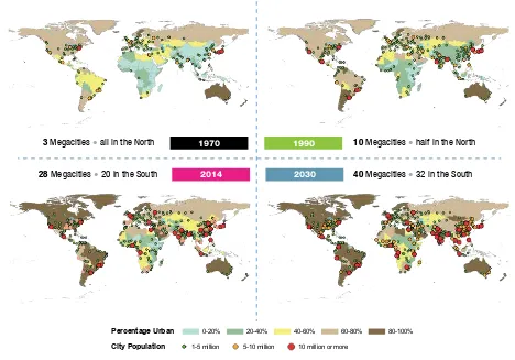
Since waste generation is significantly greater in urban than in rural areas, forecasting the split between urban and rural populations is also important. Figure 3.6 presents UN data showing the percentage of people living in urban areas by country, and also the location of cities in three size ranges above 1 million people, for four ‘snapshots’ in time. The shift from rural to urban areas since 1970 has been marked, and the projection for 2030 reinforces the trend. The only three megacities with a population over 10 million in 1970 were in Japan and the US; by 2014, there were 28 megacities, of which 20 were in the global ‘South’; by 2030, it is forecast that there will be 12 more megacities, all in the ‘South’. Urban populations are already at or approaching 80% in much of the Americas, Europe, Japan and Australia; the trend of migration to the cities still has a long way to run in Asia and particularly in sub-Saharan Africa – which coincides with the regions where total population is also forecast to continue growing most strongly.
Using these data to forecast waste arisings in individual cities in the fastest growing regions provides quite startling results. To take one example, Kinshasa in the Democratic Republic of the Congo had a population of less than 4 million in 1990, had risen to 11 million by 2014 and is forecast to reach 20 million by 2030. Allowing for increases in waste per capita with development, the total MSW generation in the city now is more than three times that in 1990, and will likely have doubled again by 2030. The challenge of providing basic MSW management services to such rapidly growing cities which are already under-served is enormous.
Unlike world population and urbanization trends, there are no authoritative UN forecasts of future waste generation per capita, and filling that gap is one of the GWMO’s recommendations for future work. As shown in
Figure 3.2, there is a clear link between waste per capita and income level; so unless specific waste prevention
measures are taken, one can assume that per capita waste generation levels in the current low- and middle-income countries will increase as their economies continue to develop and gross national middle-income (GNI) levels rise.
[image:15.595.56.524.186.513.2]Box 3.1 shows the results of a recent research project which has attempted to project MSW generation forward to 2100. It is worth repeating here the caveat that any projection beyond 2050 becomes extremely speculative. It should be interpreted as a scenario of what might happen under a particular set of assumptions, rather than a forecast of what is likely to happen.
Figure 3.6 Percentage of urban population and locations of large cities, 1970 – 2030
Percentage Urban 0-20% 20-40% 40-60% 60-80% 80-100%
City Population 1-5 million 5-10 million 10 million or more
1970 1990
2014 2030
3 Megacities • all in the North
28 Megacities • 20 in the South
10 Megacities • half in the North
40 Megacities • 32 in the South
UN disclaimer: Designations employed and the presentation of material on this map do not imply the expression of any opinion whatsoever on the part of the Secretariat of the United Nations concerning the legal status of any country territory or area, or of its authorities, or concerning the delimitation of its frontiers or boundaries.
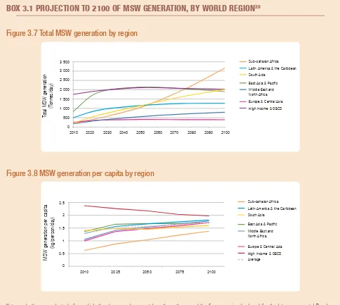
BOX 3.1 PROJECTION TO 2100 OF MSW GENERATION, BY WORLD REGION
20Figure 3.7 Total MSW generation by region
Total MSW genera
tion
(T
onnes/da
y)
0 1 500 1 000 500 2 000 2 500 3 000 3 500
2010 2020 2030 2040 2050 2060 2070 2080 2090 2100
Sub-saharan Africa
East Asia & Pacific
Europe & Central Asia Latin America & the Caribbean South Asia
Middle East and North Africa
[image:16.595.62.546.49.482.2]High income & OECD
Figure 3.8 MSW generation per capita by region
MSW genera
tion per ca
pita
(kg/person/da
y)
0 1
0.5 1.5 2 2.5
2010 2025 2050 2075 2100
Sub-saharan Africa
East Asia & Pacific
Europe & Central Asia Latin America & the Caribbean South Asia
Middle East and North Africa
High income & OECD Average
Notes: In the research study from which the above graphs were taken, the authors used the five scenarios developed for the Intergovernmental Panel on Climate Change (IPCC) that relate climate change and socioeconomic factors such as population expansion, urbanization, economic and technological development.21 The five scenarios on the shared socio-economic pathways (SSP) are: “SSP1 – Low challenges; SSP2 – Intermediate challenges, business
as usual; SSP3 – High challenges; SSP4 – Adaptation challenges dominate; SSP5 – Mitigation challenges dominate.” The scenario used for the projections shown in Figures 3.7 and 3.8 is SSP2, defined as “middle of the road, or business as usual,” in which the current trends continue and the world makes some progress towards sustainability. In that scenario, by the year 2100, population is around 9.5 billion and slightly declining. Waste per capita is linked to GNI per capita by a series of linear relationships, the gradient of which is assumed to decline over time. Five lines are used, from 2010, 2025, 2050 and 2075.
Source: Hoornweg et al. (2015). Peak Waste: When Is It Likely to Occur? Journal of Industrial Ecology, 19 (1), 117-128. http://onlinelibrary.wiley.com/enhanced/ doi/10.1111/jiec.12165/ Listed in Annex A, Chapter 3, MSW management.
While projections of outcomes so far into the future are speculative, particularly beyond 2050, they do provide some interesting insights.
Figure 3.7 shows that in the “high income and OECD” group of nations, waste generation first rises only slowly, then stabilizes and declines. As a percentage of the world total, it is declining rapidly, initially as the contribution of the two Asia regions increases rapidly, before they too stabilize. As would be expected from the previous discussion on population and urbanization, the contribution of Africa, and particularly sub-Saharan Africa, starts as relatively small, and begins to rise very quickly after 2050. What is both surprising and speculative is the forecast that Africa may become the dominant region in terms of total waste generation. Figure 3.8 provides the corresponding data for waste per capita. It should be noted that this is part input data on how waste per capita is assumed to change as GNI per capita levels rise in individual countries, and part output, back-calculated from the results in Figure 3.7 and population projections.
20 This box summarizes and provides commentary on a research project led by Daniel Hoornweg of the University of Ontario Institute of Technology. See Hoornweg et al. (2013, 2015), listed in Annex A, Chapter 3, Municipal solid waste management.
3.4
CURRENT STATUS OF MSW MANAGEMENT: PROTECTION OF PUBLIC
HEALTH AND THE ENVIRONMENT
MSW management is an essential utility service. The first steps in ensuring sound MSW management are providing a reliable collection service to all citizens and eliminating uncontrolled dumping and open burning. The world’s progress towards this target is the focus of this section.
3.4.1 Collection coverage
Providing a regular and reliable waste collection service to 100% of the urban population has been a public health objective since at least the mid-19th century. Data compiled for the GWMO from 125 countries gives the average collection coverage in low-income countries as 36% (the World Bank provides an average of 43%), lower-middle income countries 64% (World Bank 68%) and upper-middle income countries 82% (World Bank 85%), with higher income countries showing collection coverage approaching 100%. On a regional basis, collection coverage has the following ranges: Africa (25% to 70%); Asia (50% to 90%); Latin America and Caribbean (80% to 100%), Europe (80% to 100%) and North America (100%). Although these estimates are quoted as country-wide data, some incorporate the entirety of the population, both urban and rural, while others focus on urban areas. Many countries show
great variation in degree of coverage among local areas or regions. For example, the national database for Brazil gives a national average of 90.2% in 2011, but the State averages range from 60% to 99.2%.22 Similarly, in India, ministry data for 105 major cities shows collection coverage ranging from 40 to 100%.23 Because rural areas typically have lower rates of collection coverage than urban areas, national averages on collection coverage are likely to be lower than the averages of urban areas alone.
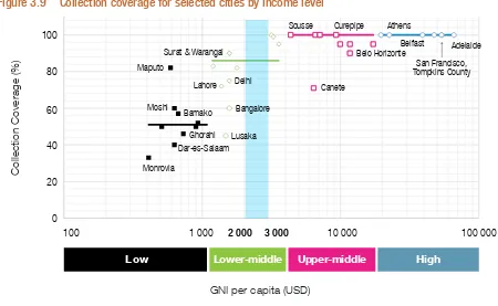
In order to assess the status of collection coverage just at the city level, Figure 3.9 shows data on 39 cities for which Wasteaware ISWM indicators are available.24Figure 3.9 appears to fall into two parts: at lower income levels, collection coverage appears to increase with increasing income, while above a certain threshold, collection reaches ‘saturation’ as levels approach 100%. If one apparent outlier (Canete, Peru) is set aside, then the threshold income level for this transition appears to lie at a GNI per capita in the range 2,000 to 3,000 USD per year. It needs to be borne in mind that data for entire cities may conceal a gap between the ‘haves’ and ‘have-nots’, in which often, the central business district and affluent neighbourhoods have near 100% coverage, while low-income and unlawful settlements often have none.
Supporting evidence comes from the 2014 comparative report for member countries of the SWEEP-Net consortium in North Africa and the Near East.25 The consortium reports collection coverage for nine countries at an average of 63%, with an average across urban areas of 75% (range 30 to 100%), and for rural areas of 40% (four at 0%, and the others at 35%, 70%, 70%, 90% and 100%).
The World Bank assessment of collection coverage quoted on their website, that “30 to 60% of all the urban solid waste in developing countries is uncollected and less than 50% of the population is served,”26 appears to be more of a reasonable historical baseline applying up to 2000 than a current estimate. If that is indeed the case, then the data presented here, both from the GWMO and from the World Bank’s own project data,27 suggests that there has been significant progress since that time, particularly in cities in those countries with an income above about 2,500 USD per capita per year (which represents approximately the mid-point in the
22 Annual reports on Brazilian waste statistics (in Portuguese). www.abrelpe.org.br
23 India, Ministry of Urban Development (2012), listed in Annex A, Chapter 3, Collated data sources.
24 Wilson et al. (2015), listed in Annex A, Chapter 2, Waste data and indicators. See also Section 2.5.3 for more information on indicators. 25 SWEEP-Net (2014), listed in Annex A, Chapter 2, Waste data and Indicators.
26 World Bank (n.d.). Urban Solid Waste Management. http://go.worldbank.org/A5TFX56L50 27 Hoornweg & Bhada-Tata, What a Waste (2012)
A resident handing over waste, India
range of lower-middle income countries). However, it is clear that many low-income cities still have collection coverage in the range of 30 to 60%, and that the figures may be much lower in some countries, and also in the more rural areas of many countries. If the figures here for collection coverage are combined with the 2014 data for world population by country income groups,28 then it can be estimated that at least 2 billion people worldwide still lack access to solid waste collection.
Figure 3.9 Collection coverage for selected cities by income level
Low Lower-middle Upper-middle High
Collection Coverage (%)
GNI per capita (USD) Monrovia
Dar-es-Salaam Ghorahi Lusaka Bamako
Moshi Bangalore Lahore Delhi
Sousse Curepipe
Belo Horizonte Athens
Belfast Adelaide
San Francisco, Tompkins County Canete
Surat & Warangal Maputo
0 20 40 60 80 100
100 1 000 2 000 3 000 10 000 100 000
Notes: Figure shows collection coverage versus gross national income (GNI) per capita on a logarithmic scale. The cities are those for which Wasteaware indicators29 were available in May 2014. The blue vertical bar represents an apparent ‘collection coverage threshold’ (GNI of 2000-3000 USD
per capita), as it was first discussed in Wilson et al. (2012). Below that threshold, collection coverage increases with income level; above the threshold, collection coverage reaches ‘saturation’ as levels approach 100%. The four coloured horizontal lines show the median collection coverage for each income group.
Source of data: Wasteaware – University of Leeds.
Waste collection services come in a wide variety of shapes and forms (Box 3.2). Services may be delivered by the formal sector, through either public- or private-sector operators, or by the community or ‘informal’ sector, through for example community based organizations (CBOs), non-governmental organizations (NGOs) or micro- and small enterprises (MSEs).30 Services may be on a relatively small scale, providing primary collection to local neighbourhoods, or on a larger scale, providing either secondary collection or an integrated collection service across the city. Pickup is carried out by a range of vehicle types, such as bicycles, tricycles, tractor and trailer, tipper trucks or purpose-build compaction vehicles, and sometimes by pushcarts or animal powered carts.31 To optimize collection systems, the use of GPS and GIS, or even route optimization software, may be relevant for large municipalities or substantial collection coverage areas.
28 World Urbanization Prospects, 2014 Edition. http://esa.un.org/unpd/wup/ 29 See Section 2.5.3 as well as Wilson et al. (2015).
30 See Section 5.6 on a financing model for delivering services.
BOX 3.2
EXAMPLES OF DIVERSITY IN MSW COLLECTION PRACTICES
Scale of operation
SMALLER-SCALE
PRIMARY COLLECTION SECONDARY COLLECTIONLARGER-SCALE
Cycle cart, India Close truck collection, Nigeria
Push cart, Vietnam Open collection, Mali
Small truck collection, China Truck collection, Spain
Primary collectors delivering waste to a secondary refuse collection vehicle, India © KKPKP © Photo courtesy: Odeniyi Ra
© Ainhoa Carpintero
© Ainhoa Carpintero © Petri Rogero © GIE Salambougou by Erica Trauba
3.4.2 Controlled disposal
Uncontrolled disposal (through open dumping and open burning) was the norm everywhere until the 1960s,32 and according to the World Bank is still the norm in most developing countries.33 This practice gives rise to substantial public health and environmental risks. These risks are significantly increased in cases in which hazardous waste is delivered to a dumpsite alongside MSW.34
The high-income countries have learned that ‘cleaning up the sins of the past’ can be significantly more expensive than disposing of waste in an environmentally sound manner (ESM).35 Legislation phasing out uncontrolled disposal was first introduced in high-income countries in the 1970s, and the standards required for ESM facilities have since been gradually raised.36
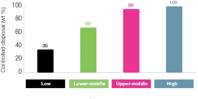
Figure 3.10 shows progress around the world in achieving the first step of eliminating open dumps and achieving
[image:20.595.149.466.322.481.2]controlled disposal, as measured by the Wasteaware controlled disposal indicator.37 This novel indicator is the percentage by weight of the residual waste remaining after collection for recycling that is received at a controlled treatment or disposal facility. ‘Controlled’ disposal involves adequate treatment of waste and operation of secured facilities so as to meet defined compliance requirements. However, a controlled facility does not necessarily have to meet the latest EU or US standards. It can also for example be an ‘intermediate’ engineered landfill or an upgraded dumpsite.38
Figure 3.10 Controlled disposal for selected cities by income level
Contr
olled disposal (wt %)
0 20 40 60 80 100
Income group
High Upper-middle
Lower-middle Low
35
68
96 100
Notes: Graph shows average percentage of controlled disposal for each of the four standard World Bank income level categories. ‘Controlled disposal’ is the primary quantitative environmental indicator defined in the Wasteaware ISWM indicator set. Data are for the 39 cities for which the indicators were available in May 2014.
Source of data: Wasteaware – University of Leeds
Phasing out uncontrolled disposal practices is one of the first objectives in improving MSW management in developing countries. Besides the 100% controlled disposal generally achieved in high-income countries, the rates in upper-middle income cities (with an average of 95%) and in lower-middle-income cities (with an average of 70%) are still substantially better than the historical ‘0% norm’. Even the average 35% in the lower-income cities is better than the historical norm. Evidence to support this apparent recent progress is given by other sources. The Brazilian national database divides disposal into three categories: sanitary landfill, which makes up 57% of the nation’s disposal on average; other landfill, at 24%; and uncontrolled dumping, at 18%. This means that in Brazil, despite relatively high controlled disposal rates, the waste from around 35 million people is dumped in an uncontrolled manner, amounting to some 15 million tonnes annually. It also suggests a comparable controlled disposal indicator likely around 80% on average. The averages for controlled disposal at
32 See Section 2.3 on drivers for waste and resource management.
33 World Bank (n.d.). Urban Solid Waste Management. http://go.worldbank.org/A5TFX56L50
34 See Box 1.2 in Chapter 1. Also, Topic Sheet 2, found after Chapter 1, provides information on ‘the 50 biggest dumpsites in the world’. 35 The costs of inaction are documented in Section 5.2.3.
36 See Sections 2.3 on waste history and Section 4.3.4 on environmental legislation. 37 See Section 2.5.3 on waste management indicators.
an individual state level range generally from 40% to 90%, with one outlier below 20%. The 2014 comparative report for the SWEEP-Net consortium in North Africa and the Near East gives controlled disposal rates in the range of 10 to 70% across nine countries, with an average of 24%. As of 2010 there were 7,518 waste disposal sites officially reported in Russia, of which around 23% were MSW landfills, 7% industrial waste disposal sites, and 70% unauthorized dumps.39 In 2011, the PRC achieved a national average controlled disposal rate of around 90%.40
A case study of the successful elimination of open dumping in a small town in Colombia is shown in Box 3.3.
In summary, the status as assessed in 2015 using the latest available data appears to be significantly better than mere dumping as the norm across developing countries. The Wasteaware data suggest that significant progress is being made by some cities in middle-income countries, with controlled disposal rates often in the range of 70 to 95%, although there is a lot of variation both within and between countries. Such achievements are impressive and compare well with the early take-up of controlled disposal in Europe in the 1970s and 1980s. The situation is much worse in low-income countries, where controlled disposal rates are often well below 50% overall and 0% in rural areas. If the figures here for controlled disposal are combined with the 2014 data for world population by country income groupings,41 then it can be estimated that at least 3 billion people worldwide still lack access to controlled waste disposal facilities.
BOX 3.3 VERSALLES, COLOMBIA: AN EXAMPLE OF INTEGRATED MUNICIPAL SOLID
WASTE MANAGEMENT
42In Versalles, a small town in Colombia, open dumping was a common sight until 1997. Through technical support from Suna Hisca, a non-profit Colombian organization, and financial support from Corporación Autonoma Regional del Valle (CVC), an integrated municipal solid waste management plan was devised. The implementation of this plan enabled Versalles to stop the contamination of its water resources and avoid potential health impacts from this practice.
The objectives of the Plan of Integrated Management of Solid Waste (PIMSW) were: (a) to achieve adequate collection, transport and disposal of municipal solid waste; (b) to engage the active participation of the stakeholders (users, the utility, the municipal administration, recyclers); (c) to get the community to practice source separation into three fractions: organics (food waste), recyclables (plastic, cardboard, metal, etc.) and sanitary waste (items contaminated with blood, urine or excreta such as sanitary towels, wound dressings, nappies, or incontinence pads); (d) to build an Integrated Solid Waste Plant to process the solid waste; (e) to create a public utility; (f) to generate employment; and (g) to improve municipal environmental sanitation. A public utility called Cooperativa Campo Verde was responsible for implementing the plan and is responsible for the collection and transportation of the waste, as well as for the operation of the plant.
As a result of the plan’s successful implementation, the rate of separation at source in 2015 was above 80%, with recoverable materials marketed and organic matter transformed into compost for sale. Of the 42 tonnes of waste generated by the community per month, 27 tonnes of organic matter and 7 tonnes of recycled materials are recovered and transformed. Overall, the town has reduced by 83% the amount of waste it would have otherwise sent to landfill. Figures 1 and 2 show the town’s new weighbridge and a new vehicle for the separate collection of solid waste.
39 IFC (2014), listed in Annex A, Chapter 3 Collated data resources 40 China Statistical Yearbook 2014, listed in Annex B.
41 World Urbanization Prospects, 2014 Edition. http://esa.un.org/unpd/wup/
3.3
RESOURCE RECOVERY
Sitting alongside the public health driver for waste collection and the environmental driver to phase out uncontrolled disposal is the resource value driver for the ‘4Rs’ – reduce, reuse,43 recycle and recover. The focus here is on recycling and recovery, of MSW in particular but not exclusively.
3.5.1 Collection for recycling
Most ‘recycling rates’ for MSW refer to the waste collected for recycling.44 Corrections are sometimes made for subsequent ‘rejects’ – materials not passed on up the materials value chain for eventual recycling – but it is difficult to audit how far corrections have been done, especially in globalized value chains of secondary materials, such as in the case of waste plastics.45 The data presented here include the collection of materials for both ‘dry recycling’ (e.g. paper, plastics, metals, glass, textiles) and organic recycling. The downstream processing of the collected waste materials
for recycling is dealt with in subsequent sections.
[image:22.595.280.512.231.500.2]Official data for MSW recycling often come from municipal governments, which in many developing countries focus on managing the MSW they collect (or which is collected on their behalf by the ‘formal sector’, leaving collection of materials for recycling often to the ‘informal sector’). Official data, either at the city level or compiled from city data by national governments, are thus likely to be under-reporting recycling rates. This was indeed one of the motivations behind the methodology developed to collect the data for the city-level Wasteaware ISWM indicators, that the system being studied should be the complete waste and recycling system for the city.46 Recycling rates were calculated with the assistance of a material flow analysis (MFA) developed for each city. Waste flows were estimated and cross-checked against each other using the MFA.47
Figure 3.11 shows the Wasteaware recycling rates from a sample of 39 cities across various income groups.
This figure shows no clear relationship between recycling rates and income levels. While recycling rates are indeed highest in the high-income countries, some low- and lower-middle income countries do collect quite reasonable percentages of their total MSW for recycling (20 to 40%). Interestingly, there is some evidence that recycling rates are lower in some of the more developed, upper-middle income countries, perhaps reflecting the history in the developed world where formalization of solid waste management as a municipal service displaced pre-existing informal recycling systems as standards of living rose, prior to the more recent ‘rediscovery’ of recycling and a resurgence in recycling rates in the high-income countries.48 More research would be required to confirm this hypothesis.
43 Both ‘reduce’ and ‘reuse’ are addressed in the Topic Sheet 4 on waste prevention, which follows Chapter 2. 44 Velis & Brunner (2013), listed in Annex A, Chapter 3, Recycling.
45 Velis (2014), listed in Annex A, Chapter 3, Global secondary materials industry. 46 See Section 2.5.3 and Table 2.3, both on indicators.
47 See Section 2.4.2 on life cycle analysis.
48 See Section 2.3.1 on historical drivers in developed countries.
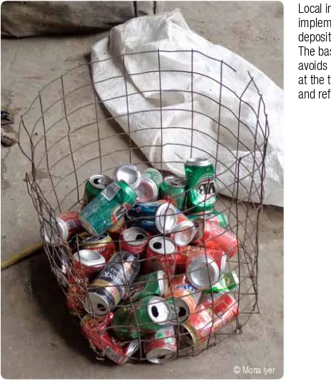
Local innovation to implement the container deposit system. The basket for 500 cans avoids manual counting at the time of deposit and refund, Kiribati
Figure 3.11 Average recycling rates for 39 cities by income level
Recycling rate (%)
GNI per capita (USD) Monrovia
Maputo Nairobi
Lusaka Sousse
Surat
Quezon City
Varna
Cigres
Bahrain Singapore
Rotterdam Belfast Adelaide Antwerp San Francisco
Tomkins County
Athens Kampala
200 100
1 000 10 000 100 000
80
60
40
20
0
Low Lower-middle Upper-middle High
Notes: Verified and consistent data from application of the Wasteaware indicators49 to benchmark recycling performance. In calculating recycling rates,
consideration has been given to both the formal municipal SWM system and any informal/community recycling being carried out in parallel (whereas ‘official’ statistics often understate recycling by ignoring the latter). The cities are those for which Wasteaware indicators were available in May 2014. Data covers both dry recyclables and organics. Where possible, correction has been made for materials collected for recycling, but ultimately disposed of after initial processing (reject fraction).
Source of data: Wasteaware – University of Leeds.
Information on recycling rates in the EU countries is now collected regularly and systematically but inconsistencies in the definition still exist (e.g. regarding counting collection for recycling vs. counting outputs of MRFs and composting plants, regarding whether or not to count metals and aggregates obtained as the output of EfW combustion plants) and the level of data reliability still differs among the EU countries. Figure 3.12 provides statistics on recycling rates in the EU countries. It may be observed that the recycling rates in the EU have increased substantially between 2001 and 2010, as the lower-performing countries have worked towards meeting the EU-wide targets.50
Figure 3.12 Municipal solid waste recycling in the European Union
http://www.eea.europa.eu/data-and-maps/figures/municipal-waste-recycling-rates-in
0% 10% 20% 30% 40% 50% 60%
70% Bulgaria Turkey Romania Croa2a
Lithuania
Slovakia
Latvia
Malta
Czech Republic
Greece
Portugal
Cyprus
Estonia Poland Hungary Iceland Slovenia Finland Spain France Italy Ireland United Kingdom
Norway Denmark Luxembourg
Sweden Switzerland
Netherlands Belgium
Germany (including Austria
MSW total recycling
2001 2010
Source: http://www.eea.europa.eu/data-and-maps/figures/municipal-waste-recycling-rates-in
49 See Section 2.5.3 as well as Wilson et al. (2015)
[image:23.595.151.416.517.714.2]3.5.2 The importance of segregation
Recycling depends critically on two aspects of ‘segregation’. The first is the degree of mixing of different elements or materials within a product, or the concentration at which the element is present, which can be addressed through design for recyclability. The second is to keep different ‘wastes’ separate at the point of generation, to ensure that they remain clean and uncontaminated by other waste streams. This can be addressed through segregation at source. These two aspects are elaborated here in turn.
[image:24.595.124.484.310.598.2]Design for recyclability
Figure 3.13 shows a plot of recyclability versus the degree of material mixing for a wide range of consumer
products. This clearly shows that products with lower degrees of material mixing are easier and more economical to recycle than others, with the degree of mixing at which recycling is feasible increasing as the value of the recycled materials rises. Products with a lower degree of mixing and higher values of the component materials are economic to recycle, while those with higher degrees of mixing and lower values are not.
One way to ‘manipulate’ this relationship is to address recyclability explicitly in the design process. For example, automobile manufacturers have recently focused on designing their products to facilitate both future dismantling (design for dismantling – DfD) and recycling (design for recycling – DfR).
Figure 3.13 Single product recycled material values
10-3
0 0.5 1 1.5 2 2.5 3 3.5
10-2
10-1
101
102
103
100
Single pr
oduct r
ecycled material value in the
United States (USD)
Material mixing, H (bits)
cantalytic converter
automobile
refrigerator automobile battery automobile tire
desktop computer work chair
laptop computer cell phone coffee maker
aseptic container PET bottle (#1)
glass bottle steel can
newspaper aluminium can
HDPE bottle (#2)
cordless screwdriver television fax machine
Apparent
Recycling
Boundary
Note: Material mixing (H) and recycling rates (for 20 products in the USA. Recycling rates are indicated by the size of the spheres: for example, automobile and catalytic convertor recycling rates are 95%, newspapers 70%, PET bottles 23% and televisions 11%. The ‘apparent recycling boundary’ separates the graph into two regions: where recycling tends to take place and where it tends not to take place. Material mixing incorporates the number of components as well as the concentrations of the components in a product, expressed as ‘H’, which is the average number of binary separation steps needed to obtain any material from the mixture (i.e. the product). For a simple product consisting of a single material only (e.g. a glass bottle), H is zero. H is therefore proportional to the complexity of the product. For instance, automobiles contain many materials and are thus more complex, so they therefore have a very high value of H. However, this graph does not indicate the actual recyclability via liberation of items by manual, mechanical or thermal processing means. Initial complexity is one thing, but the ability to liberate material is another, more critical feature.
Source: Dahmus & Gutowski (2007). What gets recycled: an information theory based model for product recycling. Environmental Science & Technology 41: 7543–7550.
all of which are either used in high concentrations and/or have a high value. Although more than half the metals have very low recycling rates of less than 1%, many of them are regarded as ‘critical materials’, including indium and gallium, or are rare earth metals including lanthanum, cerium, praseodymium, neodymium, gadolinium and dysprosium. These metals are all used in a wide range of electronic products including screens, chips and speakers and microphones and also in the magnets that are critical in many renewable energy technologies. The problem with recycling these critical metals is that the concentrations are often very low while the degree of mixing with other elements is very high. A major challenge moving forward is to ensure that design for dismantling and design for recyclability is prioritized in these rapidly growing industrial sectors.
Figure 3.14 End of life recycling rates for 60 metals
103 Lr 102 No 101 Md 100 Fm 99 Es 98 Cf 97 Bk 96 Cm 95 Am 94 Pu 93 Np 92 U 91 Pa 90 Th 89 Ac
** Actinides
71 Lu 70 Yb 69 Tm 68 Er 67 Ho 66 Dy 65 Tb 64 Gd 63 Eu 62 Sm 61 Pm 60 Nd 59 Pr 58 Ce 57 La
* Lanthanides
118 Uuo (117) (Uus) 116 Uuh 115 Uup 114 Uuq 113 Uut 112 Uub 111 Rg 110 Ds 109 Mt 108 Hs 107 Bh 106 Sg 105 Db 104 Rf ** 88 Ra 87 Fr 7 86 Rn 85 At 84 Po 83 Bi 82 Pb 81 Tl 80 Hg 79 Au 78 Pt 77 Ir 76 Os 75 Re 74 W 73 Ta 72 Hf * 56 Ba 55 Cs 6 54 Xe 53 I 52 Te 51 Sb 50 Sn 49 In 48 Cd 47 Ag 46 Pd 45 Rh 44 Ru 43 Tc 42 Mo 41 Nb 40 Zr 39 Y 38 Sr 37 Rb 5 36 Kr 35 Br 34 Se 33 As 32 Ge 31 Ga 30 Zn 29 Cu 28 Ni 27 Co 26 Fe 25 Mn 24 Cr 23 V 22 Ti 21 Sc 20 Ca 19 K 4 18 Ar 17 Cl 16 S 15 P 14 Si 13 Al 12 Mg 11 Na 3 10 Ne 9 F 8 O 7 N 6 C 5 B 4 Be 3 Li 2 2 He 1 H 1 Period 18 17 16 15 14 13 12 11 10 9 8 7 6 5 4 3 2 1 Group # 103 Lr 102 No 101 Md 100 Fm 99 Es 98 Cf 97 Bk 96 Cm 95 Am 94 Pu 93 Np 92 U 91 Pa 90 Th 89 Ac
** Actinides
71 Lu 70 Yb 69 Tm 68 Er 67 Ho 66 Dy 65 Tb 64 Gd 63 Eu 62 Sm 61 Pm 60 Nd 59 Pr 58 Ce 57 La
* Lanthanides
118 Uuo (117) (Uus) 116 Uuh 115 Uup 114 Uuq 113 Uut 112 Uub 111 Rg 110 Ds 109 Mt 108 Hs 107 Bh 106 Sg 105 Db 104 Rf ** 88 Ra 87 Fr 7 86 Rn 85 At 84 Po 83 Bi 82 Pb 81 Tl 80 Hg 79 Au 78 Pt 77 Ir 76 Os 75 Re 74 W 73 Ta 72 Hf * 56 Ba 55 Cs 6 54 Xe 53 I 52 Te 51 Sb 50 Sn 49 In 48 Cd 47 Ag 46 Pd 45 Rh 44 Ru 43 Tc 42 Mo 41 Nb 40 Zr 39 Y 38 Sr 37 Rb 5 36 Kr 35 Br 34 Se 33 As 32 Ge 31 Ga 30 Zn 29 Cu 28 Ni 27 Co 26 Fe 25 Mn 24 Cr 23 V 22 Ti 21 Sc 20 Ca 19 K 4 18 Ar 17 Cl 16 S 15 P 14 Si 13 Al 12 Mg 11 Na 3 10 Ne 9 F 8 O 7 N 6 C 5 B 4 Be 3 Li 2 2 He 1 H 1 Period 18 17 16 15 14 13 12 11 10 9 8 7 6 5 4 3 2 1 Group #
<1% 1-10% >10-25% >25-50% >50%
103 Lr 102 No 101 Md 100 Fm 99 Es 98 Cf 97 Bk 96 Cm 95 Am 94 Pu 93 Np 92 U 91 Pa 90 Th 89 Ac
** Actinides
71 Lu 70 Yb 69 Tm 68 Er 67 Ho 66 Dy 65 Tb 64 Gd 63 Eu 62 Sm 61 Pm 60 Nd 59 Pr 58 Ce 57 La
* Lanthanides
118 Uuo (117) (Uus) 116 Uuh 115 Uup 114 Uuq 113 Uut 112 Uub 111 Rg 110 Ds 109 Mt 108 Hs 107 Bh 106 Sg 105 Db 104 Rf ** 88 Ra 87 Fr 7 86 Rn 85 At 84 Po 83 Bi 82 Pb 81 Tl 80 Hg 79 Au 78 Pt 77 Ir 76 Os 75 Re 74 W 73 Ta 72 Hf * 56 Ba 55 Cs 6 54 Xe 53 I 52 Te 51 Sb 50 Sn 49 In 48 Cd 47 Ag 46 Pd 45 Rh 44 Ru 43 Tc 42 Mo 41 Nb 40 Zr 39 Y 38 Sr 37 Rb 5 36 Kr 35 Br 34 Se 33 As 32 Ge 31 Ga 30 Zn 29 Cu 28 Ni 27 Co 26 Fe 25 Mn 24 Cr 23 V 22 Ti 21 Sc 20 Ca 19 K 4 18 Ar 17 Cl 16 S 15 P 14 Si 13 Al 12 Mg 11 Na 3 10 Ne 9 F 8 O 7 N 6 C 5 B 4 Be 3 Li 2 2 He 1 H 1 Period 18 17 16 15 14 13 12 11 10 9 8 7 6 5 4 3 2 1 Group # 103 Lr 102 No 101 Md 100 Fm 99 Es 98 Cf 97 Bk 96 Cm 95 Am 94 Pu 93 Np 92 U 91 Pa 90 Th 89 Ac
** Actinides
71 Lu 70 Yb 69 Tm 68 Er 67 Ho 66 Dy 65 Tb 64 Gd 63 Eu 62 Sm 61 Pm 60 Nd 59 Pr 58 Ce 57 La
* Lanthanides
118 Uuo (117) (Uus) 116 Uuh 115 Uup 114 Uuq 113 Uut 112 Uub 111 Rg 110 Ds 109 Mt 108 Hs 107 Bh 106 Sg 105 Db 104 Rf ** 88 Ra 87 Fr 7 86 Rn 85 At 84 Po 83 Bi 82 Pb 81 Tl 80 Hg 79 Au 78 Pt 77 Ir 76 Os 75 Re 74 W 73 Ta 72 Hf * 56 Ba 55 Cs 6 54 Xe 53 I 52 Te 51 Sb 50 Sn 49 In 48 Cd 47 Ag 46 Pd 45 Rh 44 Ru 43 Tc 42 Mo 41 Nb 40 Zr 39 Y 38 Sr 37 Rb 5 36 Kr 35 Br 34 Se 33 As 32 Ge 31 Ga 30 Zn 29 Cu 28 Ni 27 Co 26 Fe 25 Mn 24 Cr 23 V 22 Ti 21 Sc 20 Ca 19 K 4 18 Ar 17 Cl 16 S 15 P 14 Si 13 Al 12 Mg 11 Na 3 10 Ne 9 F 8 O 7 N 6 C 5 B 4 Be 3 Li 2 2 He 1 H 1 Period 18 17 16 15 14 13 12 11 10 9 8 7 6 5 4 3 2 1 Group #
Notes: The figure uses the periodic table to show the global average end-of-life (post-consumer) functional recycling for sixty metals. Functional recycling is recycling in which the physical and chemical properties that made the material desirable in the first place are retained for subsequent use. Unfilled boxes indicate that no data or estimates are available, or that the element was not addressed as part of the study. These evaluations do not consider metal emissions from coal from power plants.
Source: UNEP (2011b). Recycling Rates of Metals: A Status Report. http://www.unep.org/resourcepanel/Portals/24102/PDFs/Metals_Recycling_Rates_110412-1.pdf
The presence of hazardous components is particularly important: for recycling to be economically feasible, recycling streams should ideally be contaminant free. Household hazardous waste (e.g. spent batteries), if not segregated, can contaminate the organic fractions and result in compost that is contaminated by toxic heavy metals.51 Another example is that of waste paper containing polychlorinated biphenyls (PCBs), a persistent organic pollutant (POP) that is released when some older carbonless copy papers are recycled. A 2014 study on paper and board collected from Danish household waste suggested presence of measurable quantities of PCBs that could potentially have health and environmental consequences.52
51 Velis & Brunner (2013)