Vol. 8, No. 2, pp. 858–887
A Bayesian Approach to Sparse Model Selection in Statistical Shape Models∗
Ali Gooya†, Christos Davatzikos‡, and Alejandro F. Frangi§
Abstract. Groupwise registration of point sets is the fundamental step in creating statistical shape models (SSMs). When the number of points on the sets varies across the population, each point set is often regarded as a spatially transformed Gaussian mixture model (GMM) sample, and the regis-tration problem is formulated as the estimation of the underlying GMM from the training samples. Thus, each Gaussian in the mixture specifies a landmark (or model point), which is probabilistically corresponded to a training point. The Gaussian components, transformations, and probabilistic matches are often computed by an expectation-maximization (EM) algorithm. To avoid over- and under-fitting errors, the SSM should be optimized by tuning the required number of components. In this paper, rather than manually setting the number of components before training, we start from a maximal model and prune out the negligible points during the registration by a sparsity criterion. We show that by searching over the continuous space for optimal sparsity level, we can reduce the fitting errors (generalization and specificities), and thereby help the search process for a discrete number of model points. We propose an EM framework, adopting a symmetric Dirichlet distribution as a prior, to enforce sparsity on the mixture weights of Gaussians. The negligible model points are pruned by a quadratic programming technique during EM iterations. The proposed EM framework also iteratively updates the estimates of the rigid registration parameters of the point sets to the mean model. Next, we apply the principal component analysis to the registered and equal-length training point sets and construct the SSMs. This method is evaluated by learning of sparse SSMs from 15 manually segmented caudate nuclei, 24 hippocampal, and 20 prostate data sets. The generalization, specificity, and compactness of the proposed model favorably compare to a traditional EM based model.
Key words. statistical shape models, Gaussian mixture model, sparse inference, model selection, EM algorithm, caudate, hippocampi, prostate
AMS subject classifications. 62F15, 62P10
DOI. 10.1137/140982039
Notation.
α Concentration parameter of Dirichlet distribution
π = [π1, . . . , πNM]T Vector of Gaussian priors
δ Thickness of the level set narrow bands
∗Received by the editors August 12, 2014; accepted for publication (in revised form) January 20, 2015; published
electronically April 21, 2015. The research of the authors was partially funded by the European Commission’s Framework Program 7th (contracts agreements VPH-DARE@IT ICT-2011-9-601055 and MD-Paedigree FP7-ICT-2011-9-600932) and by the Marie Skodowska-Curie Individual Fellowship (contract agreement 625745).
http://www.siam.org/journals/siims/8-2/98203.html
†Center of Computational Imaging and Simulation Technologies in Biomedicine, Department of Electronic and
Electrical Engineering, University of Sheffield, Sheffield S1 3JD, UK (a.gooya@sheffield.ac.uk).
‡Center for Biomedical Image Computing and Analytics, Department of Radiology, University of Pennsylvania,
Philadephia, PA 19104 ([email protected]).
§Center of Computational Imaging and Simulation Technologies in Biomedicine, Department of Electronic and
Electrical Engineering, University of Sheffield, Sheffield S1 3JD, UK (a.frangi@sheffield.ac.uk).
858
γj(n) Responsibility of jth model point
T={Tk} Set of K rigid transformations
X={Xk} Set ofK training point sets
Σ= diag(σ2, . . . , σ2, σ2) Covariance matrix of Gaussians
mj Position vector of jth point on M
Tk ={sk,Rk,bk} Rigid transformation mappingMto Xk
Xk={xki} kth training point set constructed fromkth shape
˜xki = [xTki, φk(xki)]T Hybrid vector of ith point onkth shape
˜xki = [xTki, φk(xki)]T] Hybrid vector ofith point onkth shape
φ(mj) Signed distance function estimated atmj
φk Signed distance function ofkth training shape
Θ ={T,M,Σ,π} Set of unknowns
D Dimension of xki
Ekij(n) Posterior ofjth Gaussian, given˜xki at nth iteration
K Number of training sample shapes
N =Kk=1Nk Total number of points on the shapes
Nk Number of points on Xk
NM Number of points on the mean model
Q(Θ|Θ(n)) Lower bound on likelihood atnth iteration
z Sparsity parameter (linear in α)
1. Introduction. Statistical shape models (SSMs), originally proposed by
Cootes and Taylor in [13], have been historically applied to the automatic segmentation of
anatomical structures [37, 36, 41, 55, 57,11,47,39,50, 28]. By exploiting statistical shape priors, these models increase the robustness of the segmentations against imperfect imaging features such as weak edges and clutter. Constructing an SSM from a training set often in-volves estimating both the mean shape and the plausible (principal) modes of its variations.
For a comprehensive review of these methods, see Heimann and Meinzer [26]. The constructed
SSM depends on the shape representation, e.g., a popular approach is binary image
repre-sentation [49,15,31, 2]. In these models, the mean shape is registered to the training sets,
usually through diffeomorphic deformation fields as nonfolding and invertible mappings. Next, to identify the modes of variations, principal component analysis (PCA) is directly applied to
either the deformation [15] or the velocity fields [31] in the tangent spaces. In a closely related
approach, Leventon, Grimson, and Faugeras [37] and Rousson, Paragios, and Deriche [48]
represented the shapes by signed distance functions (SDFs). The level set values computed over the entire image domain was concatenated into a vector and subjected to PCA. Although this method conveniently handles topological variations, nonsparse representation frequently requires large computational resources.
More compact forms of shape expression are offered by surface representation. For in-stance, in one category, the surface is expressed as a vector in a coordinate frame spanned by
a set of orthonormal basis functions. Examples include Fourier descriptors [51] and spherical
harmonics [6,33], obtained by solving the Laplace equation on a sphere. The corresponding
shape vectors are statistically analyzed by PCA. These methods were originally designed for shapes homeomorphic to a sphere and are not easily extendible to more complicated and nonconvex structures.
Shape representation using point sets has been widely reported in the literature [14, 13,
21,8,18,17] because it is simple to implement. Landmarks are sparsely chosen on the surfaces
of the training sets, and concatenated into a vector representing each shape. Evidently, the PCA outcome depends on the order of the points in the concatenation: inconsistent ordering can result in artifactual variation modes. In other words, a pointwise “correspondence” should be specified for every landmark across the training samples. In addition, the actual location of the landmarks affects the quality of PCA. Established ways of tacking these problems are
summarized in section 1.1.
Here, we estimate the number of landmarks needed to represent the mean model. This problem can be important when creating an unbiased SSM from unregistered point sets con-taining differing number of points. Intuitively, including many landmarks on the mean model increases the degree of freedom and results in overfitting in the from of loose registration (and incorrect modes of variations). Conversely, few landmarks deteriorate geometrical details. In fact, the relation between the degree of freedom in a shape model and the under/overfitting
problem is also evident in the context of geodesic active contours [10]. In its simplest form, an
evolving contour is attracted toward image edges, while its shape is regularized by penalizing its length. This leads into a curve evolution scheme that consists in a curvature weighted term
to regularize the shape of the curve [23]. Reducing the weight of curvature often results in
an unregularized curve that does not necessarily match the target borders and could overfit to image background, whereas increasing the curvature weight yields overly simplified and underfitted curves. Therefore, motivated by these observations, we hypothesize that there must exist an optimal number of landmarks (or sparsity level as discussed in the rest of the
paper) that minimizes generalization and specificity errors.1
The optimal number of landmarks should ideally minimize both generalization and
speci-ficity errors [18]. In practice, however, the errors may not be minimized by the same number
of model points. Thus, rather than obtaining an SSM with a single optimal number of land-marks, we use cross-validation and directly measure the generalization/specificity errors in the left-out samples. We then identify a range of model point numbers giving reasonable error values.
More importantly, rather than searching in the discrete space, we propose a Bayesian framework replacing the discrete number by a continuous hyper-parameter. Starting from a large number of model points, the hyper-parameter controls the sparsity rate of model point pruning during the registration. To achieve this, we formulate groupwise registration as the estimation of a Gaussian mixture model (GMM) from the training points, corresponding each model point to a Gaussian component. In this setting, the sparsity hyper-parameter defines the “concentration” parameter of a symmetric Dirichlet prior imposed on the mixture weights in the GMM. Thus, the problem of selecting the number of model points becomes that of determining the correct sparsity level. We show that this process compacts the SSMs and
reduces their generalization and specificity errors, relative to those of established SSMs [30].
In machine learning studies, estimating the number of Gaussians in a GMM is regarded as
a particular example of the “model selection” problem [16], in which models with intermediate
1The first error is related to the distance between an actual and the model predicted shapes. The latter
specifies the ability of the model to instantiate correct shapes resembling the training data.
complexity (ratio of free parameters to training data) are known to be optimal in generalization. However, to our knowledge, estimating number of model points as a particular model selection problem has not been fully considered by the medical imaging community. Here, we demon-strate that an intermediate number of model points (sparsity levels) generally improves model efficiencies. To correctly highlight the contributions of this study, we briefly review some of
the seminal SSM studies in section 1.1
1.1. Review of related state-of-the-art SSM methods. Manual selection of landmarks
and setting their correspondences across training shapes [13] can be a time-consuming and
nonreproducible procedure. In fact, landmarks are matched by machine generated approaches,
traditionally by the iterative closest point (ICP) [42] algorithm. Other automatic methods
improve the matching by including curvatures and local neighborhood features [7,54,52]. The
robustness of matchings is enhanced by spatial regularization using Markov random fields [43],
currents [53], and diffeomorphic mappings [22]. In an alternative approach, Frangi et al. [21]
extracted a set of landmarks from a preconstructed atlas and assigned each set an example shape by nonrigid B-spline mappings. However, these methods do not necessarily optimize
groupwise statistics. Regarding this problem as homologous to the minimum variance
princi-ple, Hill and Taylor [27] and Baumberg and Hogg [3] minimized the trace of the covariance
matrix by displacing the landmarks in the surface normal direction. In an alternative
ap-proach, Kotcheff and Taylor [35] minimized the determinant of the covariance matrix and
introduced a free parameter to avoid zero eigenvalues. Inspired by the Occam’s razor
prin-ciple, which favors simple models over complex ones, Davis et al. [18, 17] minimized the
length of the binary code specifying the Gaussian distribution of the data. These methods are mathematically elegant but computationally expensive, and because of their parametric surface representation, they are not readily extendible to nonspherical topologies.
Identifying correspondences between landmarks becomes even more challenging when the
training sets cannot be exactly matched [44], either because of intrinsic anatomical differences
or because the number of points differs among the point clouds. In such cases, hard-binds
established between the landmarks could introduce dummy modes in the PCA variations.
To alleviate this problem, Rangarajan, Chui, and Bookstein [45] proposed the soft-assign
procrustes algorithm for matchings two sets of landmarks with different counts. Granger
and Pennec [25] proposed EM-ICP, a combination of expectation-maximization (EM) [19]
and conventional ICP that enables partial or probabilistic matching between points. Since EM based methods can deal with complex variations, they have been popularly applied in groupwise registrations and SSM constructions.
Chui et al. [12] proposed a forward-backward consistent deformable registration of point
sets to the mean model in an EM-like framework. Their algorithm iteratively updates the point correspondences, mean model, and deformations, but it does not consolidate the results
by PCA. In a similar but computationally less expensive framework, Hufnagel et al. [30]
applied an affine transformation to register the point sets. Based on the EM outcome (i.e., the registered point clouds with partial matches between points), they then performed a heuristic PCA on the “virtually correspondent” points. Recently, Rasoulian Rohling, and
Abolmaesumi [46], replaced the affine with a B-spline based registration model, and they
applied PCA to the computed deformation fields.
In the above studies, groupwise registration of point sets was reformulated as estimating the underlying probability density function (pdf) from spatially transformed noisy observa-tions of points. The pdf is often represented as a Gaussian mixture model, whose means (estimated by EM) determine the landmark locations. Determining an appropriate number of Gaussian components for a specified number of data points, the so-called model selection problem in machine learning, is ignored in these approaches. However, model selection can avoid under- and overfitting errors and thereby improve the generalization efficiency of the trained pdf. In an SSM context, model complexity can be influenced by the number of points
representing the mean shape, which is usually selected before the training phase [25,12,30,46].
The contributions of this study are twofold. First, we propose a Bayesian framework for sparse SSM construction. Within this framework, the number of model points is indirectly
determined during the training phase. Starting from a maximal number of model points,
sparsity is enforced by employing a symmetric Dirichlet prior on the mixture weights. Neg-ligible model points are pruned during each EM iteration by a quadratic programming (QP) technique. The sparsity rate is controlled by a hyper-parameter, namely, the concentration parameter of the Dirichlet prior. As is well known, the weights of the Gaussians in the GMM become sparse when this parameter is less than unity. We optimize the value of this param-eter in cross-validation experiments and identify an approximate range that generalizes well globally over various data sets. Second, we simplify the reconstruction of surfaces from points by representing each landmark as a hybrid vector containing the level set and coordinates.
Note that our representation is denser than that of Leventon, Grimson, and Faugeras [37],
who disregarded the coordinates.
This paper extends our preliminary work in [24]. Here, we provide the mathematical
details and apply our method to different and a larger number of data sets, two of which are nonhomeomorphic to a sphere. Topologically nonspherical data pose special challenges to
training SSMs by Davis et al. [17] and Keleman, Szekely, and Gerig [33]. Thus, we compare our
method to a closely related approach proposed by Hufnagel et al. [30], which is more flexible
compared to [17,33] and has been used as a reference in an independent recent study [46].
Sparsity has been applied to SSMs by several research groups. For instance, in the sparse
shape representation of Zhang et al. [56], any unseen shape is represented by a sparse linear
combination of the training samples. Alternatively, Durrleman et al. [20] enforced sparsity
on the deformation fields using an L1-type prior, which encodes the shape variations. By contrast, our approach focuses on the number of model points.
The remainder of this paper is organized as follows. Our model is formulated in section 2.
Sections 3 and 4 present the results and conclusions, respectively. Detailed mathematical
derivations are given in the appendix (section 5).
2. Methods. This section introduces our EM algorithm. This general framework allows us to (1) align given training point clouds and (2) prune out negligible points during the
registration. The result is a sparse mean model. We emphasize that in addition to the
number of model points, the properties of the principal modes of variations affect the efficacy of the SSM. However, because of its complexity, we do not explicitly optimize the variation modes but rather obtain them by independent PCA after registration. In fact, this problem
has been extensively studied in other works, such as [17, 27, 3, 35]. Having achieved these
(a) (b)
Figure 1. Shape representation using the explained hybrid point sets: (a)Binary representation of a shape in the training set. (b)Corresponding SDF, with overlaid narrow band (shading) and zero level set contour (thick line). The shape is represented as a set of the points in the narrow band, where each point is defined by concatenating its spatial coordinates and SDF value (i.e.,˜x= [xT, φ(x)]T). The latter can aid in reconstructing the shape with the correct orientation and topology.
goals, we construct the SSM in section 2.6by determining the virtual point correspondences
[30] and applying the PCA.
2.1. Shape representation. The input data to our algorithm consists ofK binary masks,
as D dimensional images, from which we constitute our training point sets. To this end, it
is customary to sample the points from the surface of the binary masks and thus ignore the orientation of the surfaces (or the polarity of the masks). Without this information, recon-struction of surfaces from points can be handled through various approaches. For instance,
Zhao, Osher, and Fedkiw [58] first computed an unsigned distance map from the points by
solving the Eikonal equation; then a geodesic active contour was driven toward the point set using advection on the distance map. This step is time-consuming and, during its evolution, contour can be trapped in a local minima. In other related works, the direction of normal
vectors to the surface is estimated and inconsistent normal vectors are flipped [29]. Then an
SDF is constructed by moving along the normals in both directions of the surface [9]. Without
explicit information on the surface normal, its automated extraction from geometry alone is a nontrivial and ambiguous process for complex and closed structures.
Here, we take a different approach and include additional distance features on a surface’s narrow band for unambiguous surface reconstruction. As shown in Figure 1, given a binary mask we first construct an SDF, whose zero level set represents the surface of the mask.
Next, we collect all the points within a narrow band of thickness δ around the zero level
set. Each point is defined as an augmented D+ 1 dimensional vector and consists of spatial
coordinates and the corresponding SDF value. Distance information is conveyed through our EM algorithm to the constructed statistical model and can be used to infer the implied surface from the mean model. To reconstruct a surface, we first interpolate the values of the SDF on
a regular grid of voxels and then extract the zero level set (see (3.2)).
2.2. Sparsity and alignment through EM algorithm. Let X={Xk}, 1≤k≤K, denote
the set of K observed (D+ 1) dimensional training point sets defined as Xk ={˜xki ∈RD+1|
1 ≤i≤Nk}. Let φk denote the SDF from the surface of the kth segmented training shape.
The points specifying Xk are then defined as˜xki= [xTki, φk(xki)]T, wherexki = [xki, yki, zki]T specify the spatial coordinates of each point. To minimize the number of required points, we
consider only those points within a narrow band of thicknessδsurrounding the surface. Thus,
in the implementation, we have set D= 3; however, we retain the general term Din the rest
of the paper.
Let M={m˜j ∈RD+1}, 1 ≤j ≤NM, be a model point set. Similarly, each model point
can be written as m˜j = [mTj, φ(mj)]T, where mj denotes the pure spatial coordinates and
φ(mj) is the corresponding level set value at that point. In addition, letT={Tk}be the set
of K rigid transformations defined asTk={sk,Rk,bk}, which includes scaling, rotation, and
translation parameters. Each Tk globally transforms the model pointsm˜j ∈ M to the space
of Xk by
Tkm˜j ≡
skRk 0
0 sk
˜ mj +
bk 0
.
(2.1)
Now let ˜xki ∈ Xk be a noisy observation vector sampled from a Gaussian
distribu-tion centered at Tkm˜j such that p(˜xki|Tk,m˜j,Σ) =N(˜xki|Tkm˜j,Σ), where Σ = diag (σ2, . . . , σ2, σ2) is a diagonal covariance matrix. In this constraint, the variances of the spa-tial coordinates are equal but different from that of the level set values, because the spaspa-tial coordinates generally have a larger span than the level set values in the narrow bands. Since
NM points exist on M, the conditional pdf of ˜xki can be given as a mixture of Gaussians:
p(˜xki|Tk,M,Σ,π) =Nj=1M πjp(˜xki|Tk,m˜j,Σ), where π= [π1, . . . , πNM]T.
Assuming that all Nk observed points on Xk are independent, the probability of Xk can
be written as p(Xk|Tk,M,Σ,π) =Ni=1k p(˜xki|Tk,M,Σ,π). Finally, to model the pdf of the
total observation X, we further assume that the K given points sets are jointly independent
and identically distributed such that
p(X|T,M,Σ,π) = K
k=1
p(Xk|Tk,M,Σ,π).
(2.2)
Next, we estimate the set of registration parameters and the mixture coefficients through maximum likelihood and Bayesian frameworks, respectively, by maximizing the following prob-ability. The formulation is
ˆ
T,M,ˆ Σˆ,πˆ = argmax
T,M,Σ,πlog[p(T,M,Σ,π|X)]
= argmax
T,M,Σ,π[logp(X|T,M,Σ,π) + logp(π)].
(2.3)
Note the following (1) This step generates only the postregistered point sets, which are then subject to an independent PCA to obtain SSM. However, we hypothesize that an optimal registration of the point sets optimizes SSM and reduces the generalization and specificity
errors. Thus, regardless of the value ofNM, we optimize the registration parameters. (2) The
likelihood term, i.e.,p(X|T,M,Σ,π) can be infinitely large if every training point corresponds
to a model point, i.e., NM = N, 2 which is a controversial result. Therefore, we cannot
2In that case, the Gaussian components in the mixture will approach infinity and the variance will be zero.
determine an optimal NM by maximizing the right-hand side in (2.3) w.r.t.NM. To identify a suitable number of model points, we instead adopt cross-validation schemes, which quantify
those generalization and specificity errors versusNM (or the sparsity level; see section 2.3).
2.3. Prior on the mixture coefficients. In this section, we propose a prior pdf for the set
of mixture coefficients π defined in the previous section, which enables the sparse estimation
of the model points. To enforce sparsity, π is drawn from a symmetric Dirichlet distribution
function [4], given by
p(π) = Γ(NM(N(α−1) + 1)) Γ(N(α−1) + 1)NM
NM
j=1
πjN(α−1), (2.4)
where N denotes the total number of observed points (N = Kk=1Nk), Γ is the Gamma
function, and α is the concentration parameter. Note that the prior given in (2.4) is proper,
i.e., the marginalization of the prior over π is unity.
When α = 1, this distribution reduces to a uniform distribution. For α >1, distribution
is maximized when all πi coefficients equal 1/NM. However, when α < 1, the power sign
becomes negative, and the distribution prefers sparsity on the mixture coefficients, i.e., the
πi’s approach zero. Sparsity is enforced by retaining the latter condition. The lower bound
on α is determined by 1−1/NM, as explained in the next subsection.
2.4. Optimization using EM. Since, the direct solution of (2.3) does not have a closed
form, we find a tractable solution through the EM algorithm [19]. Given an estimate of the
parameters Θ = {T,M,Σ,π} at the current iteration (n), EM maximizes the lower bound
on the right-hand side of (2.3), which takes the following form:
Q(Θ|Θ(n)) = K
k=1 Nk
i=1
NM
j=1
{E(n)
kij[log(πj)
+ log(N(˜xki|Tkm˜j,Σ))]}+ log(p(π)), (2.5)
where Ekij(n) specify the posterior probability that ˜xki are sampled from the Gaussian
compo-nent of meanm˜j in the current iterationn. The EM algorithm proceeds through two iterative
steps. In the E-step, the posterior probabilitiesEkij(n) are updated using the current parameter
estimates:
Ekij(n) = π
(n)
j N(˜xki|Tk(n)m(jn),Σ(n))
NM
l=1 π
(n)
l N(˜xki|Tk(n)m(jn),Σ(n))
.
(2.6)
In the M-step, the value of (2.5) is maximized w.r.t. the unknown parameters, giving a
set of updated equations. Using the results from the last step, we sequentially update each
parameter in the following order: T,M,Σ, and π. The first set is derived similarly to the
procedures outlined in [30] and [40] (see the appendix for the details). This section focuses
on the update rule for π, the main mechanism by which sparsity is enforced.
We plug (2.4) into (2.5) and keep the relevant terms in π. We then apply the constraint
NM
j=1πj = 1 through a Lagrange multiplier λ and maximize the following expression w.r.t.
each πj, 1≤j≤NM:
Q(Θ|Θ(n)) = K
k=1 Nk
i=1
NM
j=1
{[Ekij(n)+ (α−1)]log(πj)}
+λ
⎛ ⎝NM
j=1
πj−1 ⎞
⎠+O.T.,
(2.7)
where O.T. denotes π-independent terms. Differentiating (2.7) w.r.t. πj and eliminating λ
after some algebra, we obtain
πj = γ
(n)
j +α−1
NM(α−1) + 1, (2.8)
where N denotes the total number of the observed points (N = Kk=1Nk) and γj(n) = 1/N
K
k=1
Nk
i=1E
(n)
kij. This value can be regarded as the total responsibility of model point mj
in explaining the data. When α = 1, (2.8) reduces to the classic maximum likelihood based
estimation of mixture weights with no sparsity imposed.
Note that (2.8) allows negative mixture weights because no positivity constraint is imposed
when deriving (2.7). In fact, it is easily seen that for 1−1/NM ≤ α, if γj(n) < 1−α, then
πj < 0. In other words, if the total responsibility of the model point m˜j falls below 1−α,
its corresponding mixture weight becomes negative. However, since negative probabilities are
invalid, πj of such model points is set to 0 by the QP scheme explained below. Note that
sparsity can increase when α is very close to 1−1/NM. Hence, we specify in terms of an
auxiliary variable as z ∈ (0,1), specifically α using α = (1 −1/NM)z + (1−z). In this
definition, sparsity is proportional to z.
Having estimated all πj values, we update the mixture weights by solving the following
convex optimization problem using the generalized sequential minimal optimizer proposed in [32]:
π1(n), . . . , π(NnM) = argmin π1,...,πNM
NM
j=1
(πj −πj)2
s.t.
NM
j=1
πj = 1 ∧ 0≤πj ∀j. (2.9)
Equation (2.9) effectively finds the orthonormal projection of π∗ on the space of eligible
probabilities satisfying the above conditions. At the end of the M-step, model points with
zero corresponding mixture weight, i.e., π(in), are identified and pruned out. Next, NM is
updated by counting the remaining alivepoints.
Computationally, we observed this algorithm to be very efficient. Even for a large number
of model points (NM 104), the convergence time of QP is typically less than one second.
The method breaks the convex optimization of (2.9) into a series of smaller subproblems by
identifying mixture weights that violate the constraints [32].
The model points M are initialized by a k-means algorithm [4] and all spatial
transfor-mations in Tare set to the identity transformation. The initial number of model points NM
is the total number of available points (typically N −K to avoid extreme overfitting) and is
later reduced by the imposed sparsity. The algorithm alternately iterates between the E and M-steps until convergence (in our case, this is determined by a small variation in the estimated covariance matrix). Typically, sufficiently good convergence is achieved after 50 iterations of our EM algorithm. Higher numbers of iterations produce no significant change in the results. Thus, the number of iterations was fixed to 50 in all subsequent experiments.
2.5. Brief overview of the EM-ICP method. As discussed earlier, our EM algorithm is
motivated by the study of Hufnagel et al. [30]. Besides using an affine transformation model,
the Hufnagel et al. study differs from ours in several important ways: (1) we compute the
mixture coefficients using (2.8) and (2.9), whereas the Hufnagel et al. approach assumes that
all prior probabilities of the mixture components are fixed and equal toπj = 1/NM. Hence, no
sparsity is enforced in [30] and NM must be predetermined. (2) To prevent early trapping in
local minima because of sudden drop inσ2, the variance in [30] was manually reduced by some
factor (normally between 0.8 and 0.9). We hypothesize that early drops in σ2 are prevented
by our pruning process, which removes negligible points from the model. Intuitively, we expect that the observed points are sampled from fewer Gaussian components as the pruning proceeds. Thus, the variance of such Gaussians increases to preserve the likelihood of the
observed points. (3) The number of EM iterations in [30] was user-defined. While Hufnagel
the et al. model requires three free parameters (i.e., the prespecified number of landmarks
NM, a variance reduction factor, and the number of iterations), our model requires a single
parameter (z). Therefore, the Hufnagel et al. model is more complex than our model, and its
results are more dependent on user choices.
2.6. Construction of SSM. Using the EM algorithm described in the previous section,
we first register our training data sets in X to the mean shape M by estimating the rigid
transformations in T. The resulting mean model is insufficient for predicting unseen samples.
To properly construct a generalizable SSM, we should learn the plausible shape variations that exist in the training samples. This subsection explains how the modes of variations are
computed from the registered samples. The approach, described in [30], is included here to
ensure a self-contained report.
Shape models are popularly constructed by PCA [13]. However, this method requires
one-to-one point correspondences between the aligned training data and the mean shape. By contrast, no exact point correspondences are defined in our EM-ICP based method. In fact,
point correspondences are identified by the “virtual correspondence” [30], which resolves the
problem as follows: for any model pointm˜j a virtually correspondent point, denoted by m˘kj,
is induced by the training sample Xk as
˘ mkj =
NM
i=1
Ekij
lEkljT
−1
k ˜xki,
(2.10)
where Ekij denotes the posterior probability of ˜xki being sampled from the Gaussian
com-ponent that is specified by the model point m˜j. Computing these correspondences for all
training samples, we obtain K+ 1 virtually aligned shapes (including the mean shape). Next,
each shape is columnwise concatenated to a vector, and PCA is applied to the co-variance
matrix of the shape vectors. The result is the average vector ¯x∈R(D+1)NM and the matrix
of eigenmodes P∈R(D+1)NM×n, wheren≤K is the number of principal components
consid-ered in the analysis.3 Having defined these components, any unseen sample vector x is then
computed as
x= ¯x+Pb,
(2.11)
where b is the vector of coefficients. To eliminate the noise from x, each coefficient is
con-strained by|bi| ≤3√λi, whereλi is theith eigenvalue of the co-variance matrix of the training vectors [13].
3. Results. In this section, we first describe the caudate, hippocampus, and prostate data sets and explain the construction of our training point sets from segmented structures. All the data sets are publicly available and downloadable from the repositories of MICCAI Grand
Challenges.4 Since we aimed to evaluate the quality of the statistical models themselves,
no image segmentation was performed. In fact, for comparing our SSM with the Hufnagel et al. EM-ICP model, the acquired data sets were segmented by an expert and subjected to cross-validation experiments. Therefore, we used three well-known criteria introduced by
Davis et al. [18], i.e., generalization, specificity, and compactness. For brevity, we hereafter
refer to our model as SpSSM and to the Hufnagel et al. EM-ICP model as SSM. Finally, we present the principal modes of variations extracted by SpSSM.
3.1. Data specifications. The first data set (caudate) consists of 15 segmented sets
ac-quired from subjects with schizotypal personality disorder [38]. Magnetic resonance (MR)
images were acquired by a spoiled gradient-recalled imaging protocol with the parameters,
i.e., echo time (TE) = 5 ms, repetition time (TR) = 35 ms, repetition = 1, nutation angle = 45◦,
field of view = 24 cm, acquisition matrix 256×256×124, and voxel dimensions = 0.9375×
0.9375×1.5 mm. Each caudate nucleus was manually segmented by an expert (Figure 2(a)).
The second data set contains hippocampus segmentations of both epileptic patients and healthy control individuals. T1-weighted spoiled gradient echo recalled MR images were ac-quired by two scanners with different acquisition matrices and were subsequently segmented by
experts [34]. Twenty-four data sets were randomly selected and the resolutions were unified.
The final matrix and voxel sizes were 256×256×124 and 0.781×0.781×2 mm, respectively.
Sample manual segmentations of the left and right nuclei of a single subject, used as a training
set in our experiments, are shown in Figure 2(b).
Our third data set consists of prostate structures that were manually segmented from
transversal T2-weighted MR images [1]. Data were acquired from patients with benign (e.g.,
prostatic hyperplasia) or malignant lesions. Figure 2(c) shows a sample MR prostate image
in various slices overlain by an expert segmentation. Since this data set was contributed
3The number of principle components is usually decided when the sum of the considered n eigenvalues
accounts for 98% of the total trace of the covariance matrix.
4http://www.grand-challenge.org.
(a)
(b)
(c)
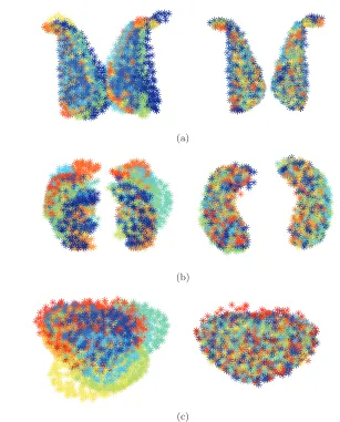
Figure 2. Sample of manually segmented slices of training data: (a) caudate nuclei, (b) hippocampal nuclei, and(c)prostate (shown in axial, coronal, and sagital slices from left to right).
by multiple centers adopting different scanning protocols, the acquired images with different resolutions. To maintain low computational burden, we chose 20 sets and resampled the expert
segmentations to element spacing of 2.0×2.0×2.0 mm. By implementing this step, we achieve a
consistent surface sampling rate across our training sets and consequently preserve the number of points generated for each individual across our populations. Naturally, this steps minimizes the possibility of artifactual bias toward oversampled or undersampled training shapes
3.2. Training point sets. For each of the caudate and hippocampus data-sets, the level
sets in the surrounding narrow bands were generated with thickness of δ = 1.5 pixels and,
approximately, 104 points per set. Next, these point sets were individually reduced to around
300 points by setting z = 0.95 and estimating no spatial transformation. Similarly, the level
sets of the prostate data sets were generated with a narrow band thickness of 1.5 mm and
approximately 3000 points per sample. In the second step, each of these point sets was
individually reduced to around 250 points by settingz= 0.7. The SSMs are constructed from
the resulting point sets in subsequent steps. Several samples of these point sets before and
following registration are shown in Figures 3(a) and3(b), respectively.
3.3. Quantitative model performance measures. Our SSM was compared to the
Hufnagel et al. model [30] in an exhaustive series of cross-validation experiments. The
gener-alization, specificity, and compactness measures were quantified for each model [18,17].
(a)
(b)
[image:13.612.143.450.89.470.2](c)
Figure 3. Registration of training point clouds by our method: (a)caudate nuclei,(b)hippocampal nuclei, and(c)prostate samples (left and right panels display the original and the registered clouds, respectively.)
The generalization performance indicates the ability of the trained model to predict unseen
test samples [18, 4]. The generalization in each fold of our cross-validation experiments was
evaluated in four steps: (1) Coregister the training set to the mean model M using the EM
algorithm. (2) Apply PCA to the coregistered training sets by (2.10) and (2.11) and compute
the matrix of eigen modes P and the mean of the registered samples ¯X. (3) Align each of the
point clouds in the left-out test set with the trained model ¯Xby reapplying the EM algorithm
but without updatingM. SetXj as the test set, which is now registered to ¯X. (4) ProjectXj
on the P space by (2.10) and (2.11) and thereby obtain X. The spatial normalization effects
on the training sets imposed by scaling, rotation and translation operations are visible in the
sample registrations shown in Figure 3. From these registered point clouds, we compute the
PCA space and project the left-out test point sets on that space.
Next, we quantify the difference between Xj (the reference point set) and ˆXj (the
model-predicted point set). The smaller the difference, the better the generalization. Following [30],
our first measure is the Hausdorff distance, defined for two given point sets as follows:
dH(Xj,Xˆj) = max{max
˜x∈Xj˜y∈minXˆjd(˜x,˜y),˜y∈maxXj˜x∈minXˆjd(˜x,˜y)}, (3.1)
where d(˜x,˜y) =||˜x−˜y||2 denotes the Euclidean distance between ˜x and ˜y. Thus, our first
generalization measure is defined as G= K1 Kj=1dH(Xj,Xˆj)
The Hausdorff distance properly quantifies the differences between details and between sharp geometrical features, such as the elongated tails of caudate nuclei. The overall similarity
of the shapes represented by X and Xj requires an alternative measure, here defined as the
average distance of the surfaces reconstructed from these point sets. To reconstruct a surface, the level set values on the three-dimensional grid of voxels are first interpolated from the scattered points by
ˆ
φ(vn) = m
φ(xm)k(||vn−xm||),
(3.2)
where ˆφ, φ are the interpolated and available level set values, k(·) is a radial basis kernel
function, and vn, xn represent the positional vectors of the query voxel n and scattered
point m, respectively. This interpolation is implemented using a fast and efficient library
[5]. Gaussian kernels were used and the bandwidth of the basis functions was set to 6 mm
and 30 mm for the caudate/hippocampus and prostate data sets, respectively. These values were retained throughout the experiments. Next, the zero level set is extracted from the
three-dimensional volume and a surface mesh is reconstructed [9].
The specificity determines the ability of the model to produce a valid output. The speci-ficity was computed by randomly sampling the SSMs within the range of valid parameters, [−3√λk,3√λk] and measuring S = R1 rR=1mink∈{1...K}dH(Xr,Xk). Here, R is the number
of randomly generated data sets,Xr is the random shape, andXkis the kth training sample.
The minimalism of the parameter set is quantified by the compactness measure, that is, the
cumulative sum of c eigenvalues of the covariance matrix of the aligned training samples,
normalized over the trace of the covariance matrix: C(c) =ck=1λk/Kk=1λk
3.4. Experiments. In this section, we compare our sparse SSM with the Hufnagel et al.
model [30]. The parameters space of both models were subjected to cross-validation
experi-ments, and the generalization, specificity, and compactness were evaluated at each point. The generalization was quantified using left-out test samples, whereas the specificity was
deter-mined from training sets. In SpSSM, the sparsity parameterzwas varied from 0.01 to 0.99 in
0.1 increments. However, the dimensions of the parameters in SSM were prohibitively large
because the NM, number of EM iterations, and variance reduction factor (section 2.5) were
freely selectable. Thus,NM was restricted to 100–3700 (approximate number of total available
points N =kNk) in increments of 400, while the other parameters were assigned typical
values.
3.4.1. Generalization. We performed threefold cross-validations on our caudate data. In each fold, 10 point sets were used for training and 5 point sets were left as test samples. We
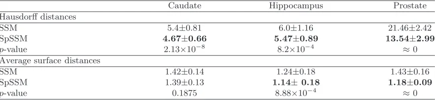
Table 1
Comparison of the minimum Hausdorff and surface distances (inmm) using SSM[30]and our sparse model (SpSSM). Measurements in bold are statistically different. The associated p-values are listed in the following rows.
Caudate Hippocampus Prostate
Hausdorff distances
SSM 5.4±0.81 6.0±1.16 21.46±2.42
SpSSM 4.67±0.66 5.47±0.89 13.54±2.99
p-value 2.13×10⁻⁸ 8.2×10⁻⁴ ≈0
Average surface distances
SSM 1.42±0.14 1.24±0.18 1.43±0.16
SpSSM 1.39±0.13 1.14±0.18 1.18±0.09
p-value 0.1875 8.88×10⁻⁴ ≈0
found that for any preselected z or NM, the EM algorithm converged to slightly different
registration results (different local minima) depending on the initialization achieved by k
-means. To minimize such randomness in the created shape models, we report the results of five experiments.
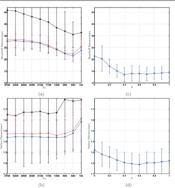
Figure 4 shows the generalization results. Evidently, the Hausdorff and surface distances
obtained by SSM depend on the number of EM iterations (specified by different colors in
Figure 4(a) and4(b)). In particular, the smallest Hausdorff distance is achieved after 15 EM
iterations; implementing more iterations does not improve the results. The distance improves as the number of model points increases to 500, but no absolute distance improvement is
observed thereafter. Comparing the results of SSM and SpSSM (Figure 4(c) and (d)), we
observe that our model reduces the errors for 0.2≤z≤0.6. The Hausdorff distance obtained
by the optimal SpSSM (at z = 0.4) 4.67±0.66 mm is significantly less than the minimum
Hausdorff distance obtained by SSM (5.40±0.81 mm) after 15 EM iterations withNM = 2500.
Table 1 summarizes the results of statistical paired t-tests of the difference analysis and the
corresponding p-values. The minimum average surface distances of the caudate data are not
significantly different between the models, suggesting that our SpSSM better captures the details (such as corners and tails), whose contributions to surface distance are attenuated by averaging, but which significantly contribute to the Hausdorff distances.
Next, we quantified the generalization by performing fourfold cross-validations on hip-pocampus data sets. In each fold, 18 sets were used for training and 6 sets were left as test
samples. To minimize randomness, which could be introduced by differentk-means
initializa-tions, we report the results of three experiments. Here, the variance reduction factor is set to
0.8 and the results are shown in Figure 5. Again, the distances computed for SSM depend on
the number of EM iterations, but more iterations do not improve the generalization efficiency
(Figure 5(a) and (b)). The Hausdorff and surface distances are minimized at 6.0±1.16 mm
(NM = 500) and 1.24±0.18 mm (NM = 1300), respectively. The results of SpSSM are shown
in Figure 5(c) and (d). The best distances of SpSSM are smaller than those of SSM when
0.1 ≤ z. In SpSSM, the Hausdorff and surface distances are minimized at 5.47±0.89 mm
(z= 0.7) and 1.14±0.18 mm, respectively. Both these errors are significantly less than their
SSM counterparts (p-values are shown in Table1).
Finally, we quantified the generalization on the prostate data sets by conducting 5 rounds of cross-validations. In each fold, 15 point sets were used for training, and 5 sets were left
3700 3300 2900 2500 2100 1700 1300 900 500 100 4 5 6 7 8 9 NM H a usdo rff D ist a n ce (mm) (a)
3700 3300 2900 2500 2100 1700 1300 900 500 100 1.3 1.4 1.5 1.6 1.7 1.8 1.9 2 NM Sur fa ce D is ta nc e( m m ) (b)
0 0.2 0.4 0.6 0.8 1
4 5 6 7 8 9 Z H a usdo rff D ist a n ce (mm) (c)
0 0.2 0.4 0.6 0.8 1
1.3 1.4 1.5 1.6 1.7 1.8 1.9 2 Z Sur fa ce D is ta nc e( m m ) (d)
Figure 4. Generalization errors obtained for15 caudate nucleus data sets (see section 3.4). Shown are the averages of 5 rounds of threefold cross validation experiments: (a) Hausdorff and (b) surface distances using the classic EM-ICP method [30] with different numbers of EM iterations (black: 25; blue: 20; red: 15; and variance reduction factor: 0.85). For comparison, the Hausdorff and surface distances obtained using our SpSSM are shown in(c)and(d), respectively. Our model reduces the Hausdorff and average surface distances (for0.2≤z≤0.6).
for testing. Figure 6(a) and (b) shows how the SSM outcomes depend on the number of
EM iterations in this data set. Comparing these to the SpSSM results in Figure 6(c) and
(d), we observe that the distances are reduced in SpSSM over the entire range of z range,
indicating better generalization by this method. The minimal Hausdorff and surface distances
are significantly smaller in the optimal SpSSM than in the optimal SSM (Table 1). The
differences between the model results are larger in the prostate data set than in the caudate and hippocampal data sets, probably because of larger variability in prostate data sets.
3.4.2. Specificity. The specificities of both models were compared by the Hausdorff dis-tances, which are more discriminative than the surface disdis-tances, as seen in the previous
3300 2900 2500 2100 1700 1300 900 500 100 3.5 4 4.5 5 5.5 6 6.5 7 7.5 NM H a usdo rff D ist a n ce (mm) (a)
3300 2900 2500 2100 1700 1300 900 500 100 0.95 1 1.05 1.1 1.15 1.2 1.25 1.3 1.35 1.4 NM Surfa ce D ist a n ce (mm) (b)
0 0.2 0.4 0.6 0.8 1
3.5 4 4.5 5 5.5 6 6.5 7 7.5 Z H a usdo rff D ist a n ce (mm) (c)
0 0.2 0.4 0.6 0.8 1
0.95 1 1.05 1.1 1.15 1.2 1.25 1.3 1.35 1.4 Z Surf a ce D ist a nc e( mm) (d)
Figure 5. Generalization errors in 24 hippocampal data sets (section 3.4). Shown are the averages of
3 rounds of fourfold cross validation experiments: Hausdorff (a)and surface (b)distances using the classic EM-ICP method [30]with different numbers of EM iterations (black: 25; red: 20; variance reduction factor:
0.8). For comparison, the Hausdorff and surface distances obtained by our sparse SSM are in (c) and (d), respectively. Our model reduces Hausdorff distance while preserving the quality of the distances (for 0.1≤z). The errors in(c)and(d)are slightly increased when the sparsity is over imposed.
subsection. Furthermore, for SSM, we consider only the EM iteration numbers and variance reduction factors yielding the best generalization outcome.
Figure 7(a)–(c) shows the specificity results for SSM. Comparing these graphs to the
corresponding specificities for SpSSM in (d)–(f), we confirm that our proposed model improves
specificity of the caudate data sets for 0.1 ≤ z ≤ 0.6 and of the hippocampal data set for
0.01≤z≤0.9. For the prostate data set, improvement is observed across the entire range of
z. Furthermore, analogous to the generalization errors in Figure 4, 5, and 6, the specificity
errors are minimized at intermediate sparsity values for all three data sets. However, the values that optimize the specificity are not necessarily those that minimize the generalization. Therefore, an optimal SpSSM model that minimizes both specificity and generalization errors is not easily determined.
3700 3300 2900 2500 2100 1700 1300 900 500 100 10 15 20 25 30 35 40 NM H a usdo rff D ist a n ce (mm) (a)
3700 3300 2900 2500 2100 1700 1300 900 500 100 1.1 1.2 1.3 1.4 1.5 1.6 1.7 NM S u rf a ce Di st a n ce( m m ) (b)
0 0.2 0.4 0.6 0.8 1
10 15 20 25 30 35 40 Z Ha u sd o rff D ista n ce (mm) (c)
0 0.2 0.4 0.6 0.8 1
[image:18.612.136.485.83.459.2]1.1 1.2 1.3 1.4 1.5 1.6 1.7 Z S u rf a ce Di st a n ce( m m ) (d)
Figure 6. Generalization errors obtained for20prostate data sets (section3.4). Shown are the averages of 5 rounds of fourfold cross validation experiments: Hausdorff(a)and surface (b)distances obtained by the EMICP method in [27] with different numbers of EM iterations (black: 30; blue: 25; red: 20; and variance reduction factor: 0.85). For comparison, the Hausdorff and surface distances obtained by our sparse SSM are shown in(c)and(d), respectively. In general, our model reduces the Hausdorff and surface distances.
3.4.3. Compactness. Figure 8 shows the compactnesses results of SSM and SpSSM. As
the sparsity parameter zincreases (asNM decreases), SpSSM (SSM) becomes more compact.
However, in both cases, models with good generalization and specificity generally have inter-mediate compactness. Although the compactness overlaps the three data sets, the proposed
sparse models with 0.1 ≤ z (for caudate) and 0.4 ≤ z (for hippocampus and prostate) are
at least as compact as SSM with adequate point counts (strong generalization performance
requires 100 < NM). Therefore, we conclude that (optimal) SpSSMs are generally more
compact than SSMs.
3.4.4. Optimality interval for sparsity parameter. Figure 9 summarizes the results of our quantitative comparisons. In this figure, for each data type we have highlighted the
ranges of z, where SpSSM outperforms SSM in various evaluation metrics. By considering
the intersection of these ranges shared across various data types, we can identify a range of
37003 3300 2900 2500 2100 1700 1300 900 500 100 4 5 6 7 8 9 NM H a usdo rff D ist a n ce (mm) (a)
33004 2900 2500 2100 1700 1300 900 500 100 4.2 4.4 4.6 4.8 5 5.2 5.4 5.6 5.8 6 NM Ha u sd o rff D ista n ce (mm) (b)
37008 3300 2900 2500 2100 1700 1300 900 500 100 10 12 14 16 18 20 22 24 26 NM Ha u sd o rff D ista n ce (mm) (c)
0 0.1 0.2 0.3 0.4 0.5 0.6 0.7 0.8 0.9 1 3 4 5 6 7 8 9 z H a usdo rff D ist a n ce (mm) (d)
0 0.1 0.2 0.3 0.4 0.5 0.6 0.7 0.8 0.9 1 4 4.2 4.4 4.6 4.8 5 5.2 5.4 5.6 5.8 6 z Ha u sd o rff D ista n ce (mm) (e)
[image:19.612.123.477.83.507.2]0 0.1 0.2 0.3 0.4 0.5 0.6 0.7 0.8 0.9 1 8 10 12 14 16 18 20 22 24 26 z Ha u sd o rff D ista n ce (mm) (f)
Figure 7. (a)–(c)Specificity errors in the caudate, hippocampus, and prostate data sets using the EM-ICP method in [30]. The corresponding errors obtained by SpSSM are shown in (d)–(f). The proposed method improves the specificities in the caudate and hippocampus data sets for 0.1 ≤ z ≤ 0.6 and 0.01 ≤ z ≤ 0.9, respectively. In the prostate data set (bottom row), the specificities are improved across the entire range z.
optimality of z, in which the proposed SpSSM is globally superior to SSM (regardless of the
data type,NM, and evaluation criterion). As seen in Figure9, this range is lower bounded at
z = 0.4 by the compactness of SpSSM on the prostate and upper bounded atz = 0.6 by the
specificity on the hipposcampus data sets. Thus, we hypothesize that a safe value forzcould
be selected in the range of 0.4≤z≤0.6 if no cross-validation experiments are considered. The
interval naturally favors models with intermediate complexities, where sparsity is in neither of extremities.
3.4.5. Sensitivity to initialization. As explained, the means of the Gaussian components
in our EM algorithm are initialized using k-means algorithm. We repeatk-means clustering
1 2 3 4 5 6 7 8 9 0 0.1 0.2 0.3 0.4 0.5 0.6 0.7 0.8 0.9 1
Modes of Variations
N o rm a li z ed C o m p a c tn ess 100 500 900 1300 1700 2100 2500 2900 3300 3700 (a)
2 4 6 8 10 12 14 16 0 0.1 0.2 0.3 0.4 0.5 0.6 0.7 0.8 0.9 1
Modes of Variations
N o rm a li z ed C o m p a c tn ess 100 500 900 1300 1700 2100 2500 2900 3300 (b)
2 4 6 8 10 12 14
0 0.1 0.2 0.3 0.4 0.5 0.6 0.7 0.8 0.9 1
Modes of Variations
No rm a li z ed C o m p a c tn ess 100 500 900 1300 1700 2100 2500 2900 3300 3700 (c)
1 2 3 4 5 6 7 8 9
0 0.1 0.2 0.3 0.4 0.5 0.6 0.7 0.8 0.9 1
Modes of Variations
N o rm a li z ed C o m p a c tn ess 0.0 0.1 0.2 0.3 0.4 0.5 0.6 0.7 0.8 0.9 1.0 (d)
2 4 6 8 10 12 14 16 0 0.1 0.2 0.3 0.4 0.5 0.6 0.7 0.8 0.9 1
Modes of Variations
N o rm a li z ed C o m p a c tn ess 0.0 0.1 0.2 0.3 0.4 0.5 0.6 0.7 0.8 0.9 1.0 (e)
2 4 6 8 10 12 14
0 0.1 0.2 0.3 0.4 0.5 0.6 0.7 0.8 0.9 1
Modes of Variations
N o rm a li z ed C o m p a c tn ess 0.0 0.1 0.2 0.3 0.4 0.5 0.6 0.7 0.8 0.9 1.0 (f)
Figure 8. Compactness, defined as the scree plots of the covariance matrices of the coaligned train-ing samples: (a)–(c) Measured by applying SSM [30] to the caudate, hippocampus, and prostate data sets;
(d)–(e) Corresponding values measured using SpSSM. The SpSSM tends to become more compact than SSM when 0.1≤z and0.3≤z are chosen for caudate/hippocampus and prostate data sets respectively. (SSMs with
NM = 100 are excluded, due to their poor generalization and specificity.)
of all data points, and then identify the best initialization by picking a k-means outcome
that has a minimal clustering cost. In order to investigate the sensitivity of the final results to initialization, we ran cross-validations measuring generalization of SpSSM under
differ-ent numbers of k-means runs. The rationale is that a robust model construction should be
0.0 0.1 0.2 0.3 0.4 0.5 0.6 0.7 0.8 0.9 z
[image:21.612.185.429.96.250.2]Caudate Hippocampus Prostate
Figure 9. Sparsity ranges where SpSSM outperforms SSM with regard to generalization (red), specificity (blue), and compactness (green) critera. As seen for 0.4 ≤ z ≤ 0.6, SpSSM is globally superior to SSM, regardless of the data type, the evaluation metric, and NM (and other parameters used to construct SSMs). Markers denote the optimal sparsity values.
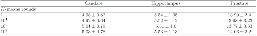
Table 2
The influence of initialization on the generalization errors (in mm) obtained by SpSSM, measured as Hausdorff distances for different number ofk-means initializing rounds (measured atz= 0.5).
Caudate Hippocampus Prostate
K-means rounds
1 4.98±0.82 5.54±1.05 13.99±3.4
101 4.92±0.64 5.52±1.12 13.98±3.23
102 5.01±0.79 5.51±1.0 13.77±3.33
103 5.03±0.78 5.53±1.13 14.06±3.2
minimally dependent on k-means outcomes. Thus, the measures should be stable across
dif-ferent numbers of initialization rounds. For these experiments, we fixed z = 0.5 and varied
k-means rounds from 1 to 103. Then we measured the Hausdorff distance of PCA projected
and original point sets as before. The results, shown in Table 2, are not statistically
dif-ferent across various numbers of k-means initializations, suggesting that our sparse model
construction is well robust to initialization.
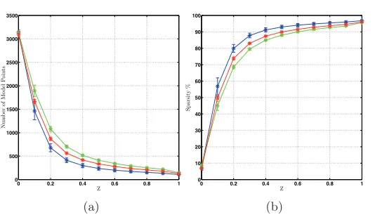
3.4.6. Nonlinear relationship between sparsity andz. Figure 10shows the relationships
between z and the number of points at convergence, and between z and sparsity levels in
the optimal SpSSM, determined by cross-validation. The converged sparsity is most sensitive
at z = 0.01 and falls almost exponentially as z increases. For instance, as z varies from 0.4
to 0.8, the sparsity of the estimated prostate model changes by less than 5%. This varying
sensitivity trend may guide the selection of z in the absence of cross-validation experiments
and measurements of the Hausdorff and surface distances.
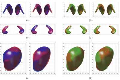
3.4.7. Qualitative descriptions. Figure 11 shows the mean models estimated by SpSSM
for different values of z. Minimal (z = 0.01) leads to anatomically incorrect models, with
several artificial structures (left panels of Figure 11). For example, unrealistic features appear
in the tails of the estimated caudate in Figure 11(a) and on the surface of the estimated
prostate in Figure 11(g). These artifacts are introduced by overfitting, which occurs when
[image:21.612.84.530.357.421.2]0 0.2 0.4 0.6 0.8 1 0
500 1000 1500 2000 2500 3000 3500
Z
Num
b
er
o
f
Mo
de
l
P
o
in
ts
(a)
0 0.2 0.4 0.6 0.8 1 0
10 20 30 40 50 60 70 80 90 100
Z
Spa
rs
it
y
%
(b)
Figure 10. Number of model points (a) and sparsity levels (b) versus z obtained in cross-validation experiments, prostate (blue), hippocampus (red), and caudate data sets (green).
(a) (b) (c)
(d) (e) (f)
[image:22.612.178.445.88.241.2](g) (h) (i)
Figure 11. Estimated mean shapes from segmented training samples(a)–(c) 10caudate nuclei atz= 0.01
(3194 points), z = 0.4 (511 points), and z = 0.99 (145 points); (d)–(f) 18 hippocampal nuclei at z = 0.01
(3149points),z= 0.7(243points), andz= 0.99(139points);(g)–(i) 15of prostate atz= 0.01(3061points),
z = 0.4 (361 points), and z = 0.99 (122 points). Arrows in the left column show the artificial structures generated by overfitting when N≈NM (section3.4).
[image:22.612.131.486.295.603.2]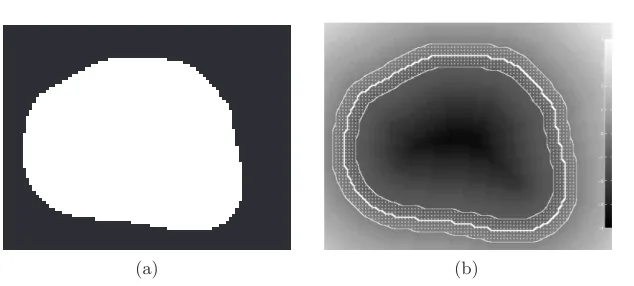
![Figure 7. andrespectively. In the prostate data set (bottom row), the specificities are improved across the entire range [30] (a)–(c).The corresponding errors obtained by SpSSM are shown in Specificity errors in the caudate, hippocampus, and prostate data se](https://thumb-us.123doks.com/thumbv2/123dok_us/7883159.184523/19.612.123.477.83.507/andrespectively-prostate-specicities-improved-corresponding-specicity-hippocampus-prostate.webp)