Dealing with numerical noise in CFD-based design optimization

This is a repository copy of Dealing with numerical noise in CFD-based design

optimization.

White Rose Research Online URL for this paper:

http://eprints.whiterose.ac.uk/79155/

Version: Accepted Version

Article:

Gilkeson, CA, Toropov, VV, Thompson, HM et al. (3 more authors) (2014) Dealing with

numerical noise in CFD-based design optimization. Computers and Fluids, 94. 84 - 97.

ISSN 0045-7930

https://doi.org/10.1016/j.compfluid.2014.02.004

[email protected] https://eprints.whiterose.ac.uk/ Reuse

Unless indicated otherwise, fulltext items are protected by copyright with all rights reserved. The copyright exception in section 29 of the Copyright, Designs and Patents Act 1988 allows the making of a single copy solely for the purpose of non-commercial research or private study within the limits of fair dealing. The publisher or other rights-holder may allow further reproduction and re-use of this version - refer to the White Rose Research Online record for this item. Where records identify the publisher as the copyright holder, users can verify any specific terms of use on the publisher’s website.

Takedown

If you consider content in White Rose Research Online to be in breach of UK law, please notify us by

1

Dealing With Numerical Noise in CFD-Based Design Optimization

C. A. Gilkeson, V. V. Toropov, H. M. Thompson, M. C. T. Wilson, N. A. Foxley and P. H. Gaskell

SUMMARY

Numerical noise is an inevitable by-product of Computational Fluid Dynamics (CFD) simulations which can lead to

challenges in finding optimum designs. This article draws attention to the issue, illustrating the difficulties it can cause for

road vehicle aerodynamics simulations. Firstly a benchmark problem is used to assess a range of turbulence models and grid

types. Large noise amplitudes up to 22% are evident for solutions computed on unstructured tetrahedral grids whereas

computations on hexahedral and polyhedral grid structures exhibit substantially less noise. The Spalart Allmaras turbulence

model is shown to be far less susceptible to noise levels than two other commonly-used models for this application.

Secondly, multi-objective aerodynamic shape optimization is applied to a fairing for a practical road vehicle which is

parameterised in terms of three design variables. Moving Least Squares (MLS) metamodels are constructed from 50

high-fidelity CFD solutions for two objective functions. Subsequent optimization is successful for the first objective, however

numerical noise levels in excess of 7% give rise to difficulties for the second one. A revision to the problem leads to success

and the construction of a small Pareto Front. Further analysis underlines the inherent capability of MLS metamodels in

dealing with noisy CFD responses.

KEY WORDS: Numerical noise, optimization, moving least squares, metamodel, CFD, aerodynamics.

1. INTRODUCTION

In the past twenty years the speed and power of computers has increased by between 1000 and 10,000 times which is facilitating the computation of increasingly complex fluid flow systems [1]. This capability is being exploited in the rapidly-growing research field of Computational Fluid Dynamics (CFD) optimization which is being utilised across a range of areas including aerospace engineering [2,3], tribology [4], polymer moulding [5], ship design [6], vehicle aerodynamics [7-10], hospital ward ventilation [11] and jet pump design [12]. Although these examples demonstrate the versatility of CFD-based optimization, there is one aspect which can prove problematic: the presence of numerical noise in the CFD responses [10,13-19].

2

beneficial, however this approach did not address the fundamental problem and no single optimum design was found. The impact of noise on response surfaces was also discussed by van Keulen et al. [14] for structural applications.

Later Madsen et al. [15] and Shyy et al. [16] commented that noise originating from numerical simulations is much less recognised than for physical experiments. An important point to appreciate is that numerical noise is an inherent by-product of computer simulation [15,24,25] and the observed behaviour is rather different from the noisy responses originating from experiments. In general, for a given physical experiment there will be statistical variation in the answer due to errors and uncertainties originating from both controlled and uncontrolled variables. In contrast, computer experiments produce the same output for a given set of input variables provided all aspects of the simulation are constant (i.e. identical initial/boundary conditions, solver version, hardware/architecture, grid structure etc.). The difference with numerical experiments is that the errors (and thus the noise) are repeatable due to their deterministic nature [18]. For optimization studies which require analysis of a wide range of designs (such as those for constructing response surfaces or metamodels) this characteristic can lead to problems in identifying optimum designs [10,13]. These issues have received attention; however, there are no studies dedicated exclusively to numerical noise and the negative impact it can have on CFD optimization. The purpose of this article is to draw attention to these in the context of road vehicle aerodynamics.

The article is structured as follows: Section 2 considers the benchmark Ahmed body [26] as a test case for simulating vehicle aerodynamics; a simple method for characterising numerical noise both qualitatively and quantitatively is presented. The influence of turbulence model selection and grid type on noise levels are discussed and analysed in detail. Section 3 describes the results from a practical high-fidelity CFD optimization problem, highlighting the difficulty of metamodel-based optimization in the face of noisy CFD responses. Section 4 draws on the results from sections 2 and 3 and strategies are proposed for minimising the negative impact which numerical noise has on optimization. Finally, conclusions are drawn in section 5.

2. NUMERICAL NOISE

Previous studies have shown that numerical noise resulting from CFD simulations is sensitive to the choice of turbulence model employed [15,16] and the grid used in the computations [17]. Burman and Gebart [17] showed conclusively that the component of numerical noise which is attributable to the grid (i.e. discretisation error) can be minimized with adequate grid resolution. Whilst these studies are helpful, there are no attempts to quantify numerical noise nor to determine the relative contributions from the known sources. The remainder of this section addresses this by assessing a range of turbulence model-grid combinations for a relevant test case.

2.1 Ahmed body

3

moving ground plane (relative to the vehicle) and rotating wheels introduce further complexity which makes the simulation of road vehicle aerodynamics a non-trivial exercise. Ahmed [26] conducted an experimental study using a generic road vehicle shape (the Ahmed body) inside a wind tunnel to characterise salient features of the time-averaged wake structure. Up to 85% of the total vehicle drag is attributable to pressure drag with over 90% of the latter resulting from flow separation over the rear faces. In the base region, the time-averaged wake structure consists of a pair of horseshoe vortices stacked vertically within the separation bubble. The strength of these vortices is found to depend on the slant angle at the rear of the vehicle. Furthermore, for high slant angles of 30º or greater, an additional but small separation bubble exists immediately behind the transverse edge joining the roof to the slanted rear face. These results are still being used as a benchmark for comparing against numerical simulations (see e.g. [29,30]). The Ahmed body is particularly relevant to the present work and it represents a suitable test case for analysing numerical noise in the context of steady-state vehicle aerodynamics simulations.

Figure 1: Illustration of the Ahmed body with relevant dimensions for a rear slant angle of = 30°.

Figure 1 illustrates the Ahmed body which consists of a solid block with rounded leading edges of radius R = 0.1m, a notch at the base and support pillars to lift the body above the ground. The size of the notch is governed by the slant angle, , which is kept constant at 30º. Other steady-state numerical studies cite poor results for smaller slant angles; when the slant angle is reduced to 25º for example, partial detachment of the flow behind the slant provides small scale structures which are inherently unsteady and these cannot be captured by steady-state approaches which often lead to poor results [31]. In order to simulate the flow field around the vehicle, a solid model was generated using Ansys Design Modeler (version 13.0) [32] based on the dimensions shown.

4

domain were assigned a zero shear stress boundary condition which is appropriate given the original open-section wind tunnel layout.

2.2 Grid structure

Recent CFD investigations of airflow past a bluff vehicle in a wind tunnel have demonstrated the importance of grid density, cell type and the choice of turbulence model for predicting aerodynamic drag [33,34]. In the present exploration three grid densities are considered for each of the following cell types: (i) hexahedral, (ii) tetrahedral and (iii) polyhedral. Each of these employ a boundary layer grid adjacent to solid walls (i.e. the vehicle and the ground) which consists of 12 layers of cells, a first cell height of 0.008m and a cell height expansion ratio of 1.2. A preliminary study showed that solutions computed using this boundary layer grid lead to average wall y+

values of between 30 and 40 on the surfaces of the vehicle which is in the correct range for the standard wall functions used [35]. Table 1 summarises each grid and Figure 2 shows the local grid structure at the base of the vehicle for the coarse hexahedral, tetrahedral and polyhedral grids respectively. The hexahedral and tetrahedral grids were generated with AnsysMesh (version 13.0) [32] and the polyhedral grids were produced using an agglomeration procedure within Fluent (version 13.0.0-sp2) [32] which converts a standard tetrahedral grid into an equivalent polyhedral one.

Global Cell Count

Grid type Local grid spacing (m) Hexahedral Tetrahedral Polyhedral

Coarse 0.015 229512 396106 173934

Medium 0.010 479865 703887 302074

Fine 0.007 699314 1383917 583475

Table 1: Grid statistics

Figure 2: Local grid structure on the symmetry plane (dark cells) and the rear of the Ahmed body for (a) hexahedral, (b) tetrahedral and (c) polyhedral cells.

2.3 Turbulence models

5

namely: (i) the Spalart Allmaras model (SA) [36], (ii) the realizable k- model (RKE) [37] and (iii) Menter’s shear-stress-transport k- model (SSTKO) [38].

Steady-state solutions were computed using Fluent (version 13.0.0-sp2) [32] for each turbulence model on all 9 grids, giving 27 solutions in total. All solutions assumed a free-stream velocity of 60 m/s and turbulence intensity of 0.5% at the inlet [26] (Note that the relatively high inlet velocity is to compensate for the reduced scale of the vehicle which leads to a Reynolds Number of 4.3 million and is consistent with the original experiments [26]). Irrespective of the turbulence model-grid combination, every simulation employed second order discretisation of the flow equations in conjunction with the SIMPLE [39] pressure-velocity coupling algorithm. Although solution convergence was generally achieved in fewer than 1000 iterations, all simulations were run for a total of 5000 iterations to eliminate convergence errors.

2.4 Quantifying numerical noise

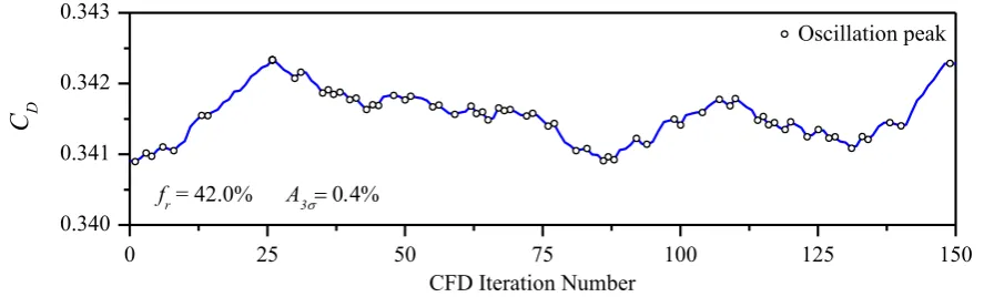
For each of the simulations described above, the drag coefficient of the vehicle, CD, was monitored throughout the 5000 iteration cycle. In all cases numerical noise was evident, characterised by a combination of structured periodic cycles with seemingly random oscillations superimposed. Interpreting these characteristics is difficult from visual inspection alone and so there is a need to quantify the noise levels. Figure 3 shows a typical noise sample from one of the simulations, taken from iterations beyond the point of solution convergence.

Figure 3: Sample of numerical noise exhibited by a Spalart Allmaras solution on the fine hexahedral grid.

The noise levels can be decomposed into the frequency and the amplitude of oscillation. The former is conveniently defined by the percentage oscillation frequency, fr, given by:

n f

n

i i

r







 0

100 , (1)

where i is the oscillation parameter evaluated for the i th

iteration for a sample size of n iterations. If CD increases monotonically from one iteration to the next, = 0. For a maximum or minimum point (i.e. oscillation peak in Figure 3) the sign of the gradient dCD/di changes and = 1. It follows that for fr = 0 the signal is likely to be stable with no oscillations present, whereas fr = 100 indicates a fully oscillatory signal where the gradient changes sign every iteration. It should be noted that fr accounts for all local gradient changes but it does not

0 25 50 75 100 125 150

0.340 0.341 0.342 0.343

f_r = 42.0% A_3

C

CFD Iteration Number

6

consider low-frequency oscillations (e.g. on the order of 100’s of iterations). As CFD solutions for steady state problems are typically taken from the final iteration, low-frequency oscillations are far less influential and thus less relevant than the high frequency ones described by fr.

In addition to the frequency, the amplitude of each individual oscillation accounts for the magnitude of the variations present. For a given sample size, three standard deviations, 3 , (known as the three-sigma rule in statistics), is an adequate measure of the data spread because it accounts for 99.7% of the values recorded. This is used to define the percentage amplitude of noise, A3 , (for the sample) relative to the mean value, namely:

D

C

A3 1003



where is the standard deviation andC_D is the mean drag coefficient for a sample of size n. As with fr, small

values of A3 denote less noise whereas larger ones signify a noisy response. For the 150-iteration sample shown in Figure 3, fr = 42.0% and A3 = 0.4%; i.e. the noise is frequent but its impact is minimal because of the small amplitude.

2.5 Impact of grid type, cell type and turbulence model

The parameters defined by equations (1) and (2) are used to analyse the numerical noise present in the data obtained for CD for the range of iterations: 2500-5000, per simulation. A sensitivity study showed that this sample size is large enough to adequately characterise both fr and A3 and it only considers the converged region

of each solution. Table 2 summarises these parameters along with the mean drag coefficient, C_D , for the range

of grid-turbulence model combinations tested. In all cases the computed drag coefficients are less than the equivalent experimental value of 0.378 [26]. Overall the SA model gives the most satisfactory result with the RKE and SSTKO models generally exhibiting the smallest drag values. The computed drag coefficients generally reduce as the grid density increases regardless of the turbulence model. As mentioned previously, Reynolds-Averaged Navier-Stokes (RANS) equations such as those employed in this study do have their limitations [31], however the results obtained are in reasonable agreement with physical experiments, and the primary focus here is on numerical noise.

SA RKE SSTKO

Grid type Cell type C_D fr (%) A3 (%) C_D fr (%) A3 (%) C_D fr (%) A3 (%)

Coarse Hexahedral 0.368 55.7 0.1 0.339 79.1 0.1 0.309 14.5 1.6

Medium Hexahedral 0.353 8.6 0.2 0.313 13.8 0.0 0.298 24.0 1.1

Fine Hexahedral 0.341 39.2 0.4 0.342 41.4 0.5 0.300 13.2 1.6

Coarse Tetrahedral 0.367 95.1 0.4 0.377 9.4 22.6 0.324 28.0 7.6

Medium Tetrahedral 0.354 100.0 0.0 0.308 16.3 2.3 0.304 39.8 0.0

Fine Tetrahedral 0.351 96.2 0.8 0.317 75.2 8.3 0.332 76.4 7.2

Coarse Polyhedral 0.354 100.0 0.0 0.318 49.8 0.0 0.327 100.0 0.0

Medium Polyhedral 0.346 2.6 0.1 0.302 39.8 0.0 0.309 9.2 5.1

7

Table 2: Computed mean drag coefficients and associated numerical noise as a function of grid type, cell type

and turbulence model. Note: from [26] the experimental drag coefficient,

C



0

.

378

It is interesting to note that both fr and A3 vary considerably, depending on the grid and cell type and the turbulence model; clearly all three factors impact the noise levels which is consistent with earlier studies [15-17]. The differences in the observed values of fr illustrate that the noise levels are not in phase from one simulation to another. In terms of the amplitude of oscillations they are below 1% for all SA solutions, however variations as high as 22.6% and 7.6% are present in the solutions for the RKE and SSTKO models respectively. Clearly, the choice of turbulence model is instrumental in determining the noise levels for this particular application.

In the majority of cases the frequency and the amplitude of oscillations are greatest for solutions computed on the tetrahedral grids compared to the hexahedral and polyhedral ones. , however there is no apparent correlation with the grid density. In some cases the noise amplitude increases as the grid becomes finer, e.g. SA solutions on the hexahedral and polyhedral grids. However, for the remaining cases the largest amplitudes (per combination of cell type and turbulence model) can occur for either the coarse, medium or fine grid densities. Whilst there is a lack of generality for these results, the fine-grid solutions are inevitably closer to being grid independent and so these are more relevant to the overall discussion.

2.6 Fine-grid solutions

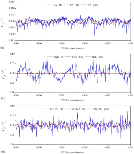
Figure 4 shows a 500-iteration sample of the relative drag coefficient (with respect to the mean value,C_D) as a

8

Figure 4: Plots of the relative drag coefficient (C_D/C_D ) as a function of steady-state iteration number per grid

cell type for (a) SA, (b) RKE and (c) SSTKO turbulence models. Note the smaller y-axis scale for (a).

The disparity in results between respective turbulence models is particularly noteworthy, especially when considering that the same grids and initial/boundary conditions are used throughout. One possible reason for this is that solutions produced by certain turbulence models may have large discretisation errors due to inadequate grid resolution. To investigate this, the Grid Convergence Index (GCI) [40] was employed to estimate the fine-grid discretisation error, GCIFINE, namely:

4000 4100 4200 4300 4400 4500

0.985 0.990 0.995 1.000 1.005 1.010 1.015

4000 4100 4200 4300 4400 4500

0.90 0.95 1.00 1.05 1.10

4000 4100 4200 4300 4400 4500

0.90 0.95 1.00 1.05 1.10

SA - tet SA - hex SA - poly

C D

/

C D

CFD Iteration Number

RKE - tet RKE - hex RKE - poly

C D

/

C D

CFD Iteration Number

(c) (b)

SSTKO - tet SSTKO - hex SSTKO - poly

CD

/

CD

CFD Iteration Number

9

 

_

_

1

100

%





r

e

F

GCI

where FS is the factor of safety, r is the grid refinement ratio (based on local grid spacing), p is the order of discretisation and e is given by:









 . (4)

For this study p = 2 (i.e. second order), r = 1.5 and FS = 1.25 based on the recommendations of [40,41]. It is clear that the discretisation errors vary significantly depending on the turbulence model and the grid cell type, see Table 3.

GCIFINE (%)

Cell type SA RKE SSTKO

Hexahedral 3.4 8.4 0.7

Tetrahedral 0.9 3.1 8.4

Polyhedral 0.6 2.0 3.2

Table 3: Discretisation errors calculated for the fine-grid solutions using the Grid Convergence Index (GCI) [40].

Overall, the errors are small for the SA model which may explain the small noise levels shown in Figure 4a. Similarly, larger discretisation errors are evident for both the RKE and SSTKO models which correspond with the larger noise levels present in Figures 4b and 4c, respectively. Thus, on the whole, the lower the discretisation error, the smaller the level of numerical noise present in the solutions.

2.7 Impact of noise

It is clear from the results presented thus far that numerical noise can dramatically influence CFD solutions. Previous studies by Madsen et al. [15] and Forrester et al. [19] have highlighted the impact this can have when plotting functions of interest through a design region. The former study focussed on an extremely small segment of the design space where the CFD responses were oscillatory yet they should have shown a linear variation; noise levels of 1.0% were found to be responsible. This problem occurs because CFD solutions are typically taken from the final iteration (for steady state simulations) and this could correspond with any region of the noisy response. As some solutions will coincide with noise peaks and others nearer the mean value, each solution is essentially iteration dependent.

10

these two turbulence model-grid combinations produce both extremes of noise, they are suitable for investigating iteration dependency for small changes in . Corresponding simulations were run for 5000 iterations with the

mean value for the drag coefficient,C_D , taken for the interval 2500-5000 iterations (as before) and the final

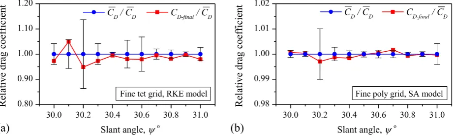
value,C_Dfinal, taken from the last iteration. Figure 5 shows how C_Dfinal (normalised with respect to C_D )

varies as a function of for both cases. The variations are clearly seen when compared to the mean relative drag

coefficient (C_D/C_D) which has error bars determined from the noise amplitude, A3, per simulation.

Figure 5: Plots of the relative drag coefficient in terms of the mean (C_D/C_D ) and the final iteration value (

D final

D

C

C

/

Figure 5a underlines the inherent variability of solutions computed using the RKE model in combination with tetrahedral-based grids. As an example, for = 30.2º the spread of solution values due to numerical noise is ±13.6% (based on A₃). More importantly, in a number of cases the range of final iteration solutions vary

considerably from the mean: e.g. for = 30.1º the final iteration value, C_Dfinal, is almost 5% greater than the

mean. Thus these iteration dependent solutions skew the final result by a considerable margin and the root cause of the discrepancy, numerical noise, should be treated with caution in other investigations.

For the low noise case (Figure 5b), solutions computed on the polyhedral grid using the SA model lead to significantly smaller noise levels with a maximum spread of 1% observed for = 30.2º. In terms of the final iteration values, the largest discrepancy also occurs for = 30.2º with a solution 0.3% below the mean; however, discrepancies of 0.1% are typical. Another aspect of Figure 5 which deserves attention is the variation in noise levels observed between geometries, especially given the small (one-degree) range of slant angles considered. This shows that noise levels are sensitive to the exact geometry and this is particularly relevant to design optimization which typically requires solutions for a range of geometries.

30.0 30.2 30.4 30.6 30.8 31.0 0.80

0.90 1.00 1.10 1.20

30.0 30.2 30.4 30.6 30.8 31.0 0.98

0.99 1.00 1.01 1.02

C_D / C_D C_D-final / C_D

R el at ive dr ag coe ff ic ie nt

Slant angle, o

Fine tet grid, RKE model Fine poly grid, SA model

C_D / C_D C_D-final / C_D

R el at ive dr ag coe ff ic ie nt

Slant angle, o

11

3. CFD-BASED OPTIMIZATION

The results presented above for the Ahmed body provide valuable insight into numerical noise and its impact on CFD solutions. Major contributing factors include the choice of turbulence model, the grid density and cell type. In combination, these three factors can lead to significant noise levels which dramatically affect solution values from iteration to iteration. While the Ahmed body represents a valuable test case, this is a simple, constrained geometry. As described in section 1, numerical noise can be extremely problematic in the context of design optimization which often requires CFD solutions for multiple geometries. As well as highlighting the problems associated with numerical noise, the purpose of this article is to show how noise levels can impact design optimization and to establish ways of dealing with it. Considered below is the effect this can have as part of an optimization problem for a practical engineering investigation.

3.1 Small livestock trailers

In the United Kingdom the majority of animals transported between farms, markets and abattoirs are carried in small box-shaped livestock trailers such as the one depicted in Figure 6.

Figure 6: Illustration of a small livestock trailer and towing vehicle.

12 3.2 Problem formulation

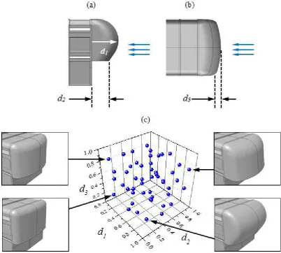
The proposed fairing is parameterised in terms of three design variables, namely the side radius, d1, the lower edge extension, d2 and the central extension of the fairing, d3, see Figures 7a and 7b. The purpose is to apply aerodynamic shape optimisation in satisfying the following criteria:

min F1 (d) and max F2 (d), (5)

where d di diU, i1,2,3 L

i ; (6)

F1 and F2 are the objective functions for the aerodynamic drag coefficient (dimensionless) and the ventilation

rate (m3/s) respectively and di is the ith design variable subject to relevant lower (d_iL) and upper (d_iU) physical

constraints.

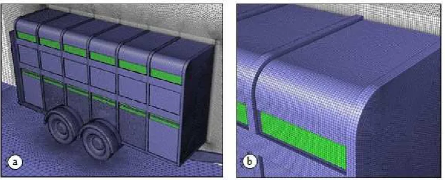
Figure 7: Parameterisation of the headboard fairing viewed from (a) the side and (b) above the trailer and (c) plot of the Design of Experiments (DoE) together with four sample fairing designs.

13

The optimization procedure involves building metamodels for each objective function (F1 and F2) and then optimizing on these to obtain a Pareto front from which to determine the optimum fairing design. To achieve this, each metamodel is fitted to CFD responses from fifty fairing designs which are chosen by an Optimal Latin Hypercube (OLH) Design of Experiments (DoE) [44]. Figure 7(c) depicts the DoE and four sample fairings which exist within the design space. Though not immediately obvious from Figure 7(c), one of the defining characteristics of the DoE is the uniformity of point coverage which is governed by the Audze-Eglais potential energy criterion [45,46].

Steady-state CFD solutions to the governing incompressible Navier-Stokes equations were used to assess each fairing by obtaining values of F1 and F2. A preliminary grid independence study carried out on the baseline trailer (Figure 6) showed that a hybrid hexahedral-tetrahedral grid consisting of 6.7 million cells led to small discretisation errors (equation 3) of 1.5% and 2.0% for F1 and F2, respectively [10]. As shown in section 2, solutions computed on both hexahedral and polyhedral cell types lead to reduced noise levels compared to tetrahedral cells. In practice, hexahedra are easier to implement than polyhedra and they are less susceptible to numerical diffusion. For this reason hexahedral cells were placed in as many regions of the solution domain as possible which included a structured boundary layer grid adjacent to the primary livestock trailer surfaces. Inevitably tetrahedral cells were required in the remaining volume due to the geometric complexity which illustrates one of the difficulties of practical CFD application. Despite this, the results from section 2 show that the noise amplitudes for solutions computed on fine grids using the SA model are 0.4% and 0.8% for hexahedra and tetrahedral respectively. As the SA model is used in this section (the justification is explained in the next paragraph) the negative impact of tetrahedral cells is relatively small. Figure 8 shows the local grid structure in the vicinity of the baseline trailer with the symmetry plane visible in the background.

Figure 8: Illustration of the local grid structure (a) surrounding the trailer and (b) near the foremost upper vent opening.

14

6) verified that this model performs more satisfactorily than both the SSTKO and RKE models. Furthermore, the SA model has been shown to produce accurate results when validated against wind tunnel experiments of a 1/7th scale livestock trailer [33], and this was selected together with QUICK [48] discretisation. Computations were carried out using Fluent [32] for a total of 10,000 iterations and convergence of all quantities was observed after 9000 of these, thus ensuring that no inaccuracies were present due to convergence error. The greater detail contained within this geometry required finer grids than those used for the Ahmed body (considered in section 2) which is why a larger number of iterations was required to reach convergence. The important point is that the solutions were converged.

3.4 Optimization strategy 1: final value solutions

Having obtained all fifty sets of CFD solutions, metamodels were built for each objective function using the Moving Least Squares (MLS) method [48,49] within HyperStudy (version 8) [50]. This technique caters for noisy responses by selecting an appropriate closeness of fit parameter, , which is contained within a Gaussian weight decay function, namely:





exp _j

j r

w   , (7)

where rj is the Euclidean distance of the metamodel prediction location from the j th

DoE point [49]. High noise-smoothing is achieved if is small because the fit is loose due to the approximation whereas high values of lead to interpolation and no smoothing. Each metamodel was tuned to give the optimum value of to ensure the best fit to the CFD responses, see [10] for more details.

For each CFD simulation, responses for F1 or F2 were taken from the final iteration. Satisfying the second objective of maximizing ventilation proved difficult because all fifty fairing designs resulted in poorer ventilation with respect to the baseline case (i.e. no fairing present). Further analysis showed that the presence of any given fairing streamlined the front of the trailer which guided airflow past the vents instead of through them thereby reducing the ventilation rate. Consequently, maximizing ventilation (equation 1) is not feasible with the current problem formulation. Instead, the second objective was changed such that the percentage reduction in ventilation rate could be minimized (min F2 (d)) which is equivalent to minimising the negative impact that the fairing has on ventilation [10].

In order to find a fairing design for minimum drag (i.e. min F1 (d)), a Genetic Algorithm (GA) was employed to carry out a global search on the corresponding metamodel before using a local gradient search

method, the Sequential Quadratic Programming (SQP) technique, to ‘home in’ on the proposed global minimum.

15

Figure 9: Objective function plot for a range of fairing designs based on final value CFD solutions.

The above optimization procedure was repeated for the ventilation metamodel in search of an optimum ventilation fairing. This proved to be problematic because the optimizer repeatedly predicted a fairing which was poorer than many of the DoE points. Nevertheless the design, which resides in another corner point of the parameter space, was tested with a CFD simulation. The result concurred with the metamodel in showing that the

design exhibits poor performance, see “Max-Ventilation” label in Figure 9. Subsequent metamodel rebuilding with the additional data point made no difference to the predicted global optimum. In an effort to construct a Pareto front with the possibility of finding better ventilation designs, four additional points were suggested by the metamodel. Each of these was found by placing a constraint on F1 to give F2 for each design [10]. CFD solutions were obtained for each but the poor results shown in Figure 9 (see “Extra Points”) underline the difficulties of optimizing the fairing for ventilation.

3.5 Optimization strategy 2: mean solutions

The presence of numerical noise in each CFD solution for F2 was suspected as the root cause of the difficulties encountered above. This is explored in Figure 10a which shows a typical solution history where the drag coefficient, CD, and the ventilation rate, Q, are plotted as a function of the iteration number. Closer inspection of

CD over the converged portion of the data (Figure 10b) shows that the noise frequency is relatively high at 36.7%, although this is accompanied by a small amplitude of 0.6% (i.e. ± 0.3%). In contrast, Q, which is used in the calculation of F2, exhibits lower frequency noise of 1.3%, however, the amplitude is large at 7.0%.

This result underlines the inherent variability of solutions for F2 and the potentially large discrepancy between mean and final value CFD solutions. In light of this fact, the difficulties in optimizing F2 are unsurprising. A possible way of avoiding these problems is to mask the noise by building metamodels using

0.495 0.500 0.505 0.510 0.515 0.520

0 10 20 30 40 50

DoE Points Min-Drag Max-Ventilation Extra Points

F 2

(%)

16

mean values which eliminate possible data spikes. Accordingly, each CFD solution was run for a further 2000 iterations and the mean for F1 and F2 calculated. Both metamodels were updated using this revised data and the optimization procedure repeated (as above) in search of min F1(d) and min F2(d). As before, optimization identified the same optimum fairing for F1, however, the same sub-optimal design was predicted for the second objective function, F2, see “Max-Ventilation” point in Figure 11. Although some of the “Extra Points” show improvement in terms of drag (compared to Figure 9), the problems relating to F2 persist and optimization of this function was not successful using our approach.

Figure 10: Plots showing typical noise levels for one CFD solution.

0 2000 4000 6000 8000 10000 12000

0.0 0.1 0.2 0.3 0.4 0.5 0.6

C_D Q

CFD Iteration Number

CD

0.0 0.1 0.2 0.3

Q

(m

3 /s

)

8000 9000 10000 11000 12000

0.511 0.514 0.517

(b)

C D

8000 9000 10000 11000 12000

0.22 0.24 0.26

f_r= 36.7% A_3= 0.6%

(c)

Q

(m

3 /s

)

(a)

17

Figure 11: Objective function plot for a range of fairing designs based on mean value CFD solutions taken from 2000 iteration cycles.

3.6 Optimization strategy 3: problem revision

The results in Figure 11 show that simply masking pronounced noise levels using mean solutions does not remedy optimization problems. Instead, the reliability of the objective function for characterising ventilation was investigated. Whilst ventilation is a suitable measure of the air quality within the trailer, its calculation is based on 2D surface integrals of the volumetric flow rate through each of the side vents in the lower deck (Figure 6). As these regions are oblique to the free-stream, large flow gradients are present and this leads to the high noise levels cited above. Further investigation revealed that the vent openings experiencing the greatest flow gradients produced the highest variability (and thus noise) from iteration to iteration as each solution progressed. By basing the objective function on a 3D volume-averaged quantity, the impact of high flow gradients reduces substantially. Consequently, the temperature humidity index (THI) [51], which has units of ºF, was chosen. This is given by the relation:



 









 Tdb rh Tdb

THI

(8)

where Tdb is the dry bulb temperature (ºC) and rh is the relative humidity expressed as a percentage. By taking the volume-average of this quantity throughout the lower deck of the trailer, thermal comfort and thus animal welfare is considered instead of ventilation. Accordingly the problem was revised to:

min F1 (d) and min F3 (d), (9)

0.500 0.505 0.510 0.515 0.520 0.525

0 10 20 30 40 50

DoE Points Min-Drag Max-Ventilation Extra Points

F 2

(%)

18

where F3 is the objective function representing THI. Using the isothermal solutions as a basis, all simulations were run for an additional 4000 iterations with extra transport equations for energy and species also solved; these account for thermal effects and humidity, respectively. Source terms for energy and moisture production were used to represent animal warmth and perspiration so that F3 could be calculated for hot (30 ºC) and humid (rh = 95%) ambient conditions (see [10] for more details). With these new parameters incorporated into the CFD simulations, convergence was observed within the first 1500 iterations and so the means for F1 and F3 were calculated from the remaining 2500 iterations.

Results from the revised simulations were found to be free of significant noise levels, justifying the problem revisions. Table 4 summarises the noise statistics for all 56 simulations with mean amplitudes of 0.3% and 0.2% evident for F1 and F3, respectively. Overall, the noise frequency is greater in the results for F3; however, the small amplitudes present for both objective functions underline the dramatic improvement; this is in complete contrast to the noisy responses seen earlier.

F1 F3

Value fr (%) A3 (%) fr (%) A3 (%)

mean 4.6 0.3 15.6 0.2

max _{10.8 6.5 33.0 0.6}

min 1.7 0.1 1.5 0.0

Table 4: Noise statistics for all 56 simulations obtained using the problem revision.

In addition to the reduced noise levels, the “Extra Points” generated in the previous section show a considerable improvement in terms of the second objective function, in this case F3. This is evident in Figure 12a which displays all 56 points based on final value solutions. In terms of mean values the objective function plot retains the same features with all 56 points residing in broadly similar locations, see Figure12b. As mean values are more representative of the actual solutions, these were used to construct new metamodels from the revised data prior to optimizing. The drag metamodel predicted the same optimum fairing design as before, whereas the THI metamodel revealed a candidate for min F3(d). An additional CFD simulation verified that this design gave the smallest THI of all the designs tested, suggesting that the optimum for F3 had been found, see “Min-THI” in Figure 12b. This conclusion was verified from subsequent metamodel rebuilding and optimization with the additional point; it did not lead to a better design. Note that the small Pareto front was generated using a multi-objective genetic algorithm (MOGA) [52] which was applied to both metamodels. Although this did suggest a

19

Figure 12: Objective function plot for the revised problem using (a) final values and (b) mean quantities including the minimum-THI design and Pareto front.

3.7 Advantages of Moving Least Squares metamodels

Of all the data points shown in Figure 12, the locations of the “Extra Points” are particularly noteworthy. These four designs were predicted in the isothermal optimization (section 3.4) yet they exhibited sub-optimal performance in terms of ventilation and drag. With the above problem revision these very same designs now reside in the most promising region of the objective function landscape and, in terms of mean solutions, one of them is in fact Pareto optimal. Therefore, in spite of the pronounced noise levels seen in the isothermal study, the MLS metamodelling technique was in fact successful in filtering this noise and thus identifying optimal design

0.48 0.49 0.50 0.51 0.52

85.9 86.1 86.3 86.5 86.7 86.9

0.48 0.49 0.50 0.51 0.52

85.9 86.1 86.3 86.5 86.7 86.9

Baseline DoE Points Min-Drag Max-Ventilation Extra Points Min-THI

MOGA Pareto Front

F 3

(



F

)

F

(b)

Baseline DoE Points Min-Drag Max-Ventilation Extra Points

F 3

(



F

)

20

characteristics. It follows that the MLS metamodels in this study were in fact more accurate than the high-fidelity CFD solutions used in the initial problem formulation. This stems from the inherent noise-handling capability of the approximation-based technique employed and is consistent with the earlier findings of Papila and Haftka [53].

3.8 Optimum design

Taking the results from Figure 12 into consideration the “Min-THI” design was chosen as the overall optimum; it produces the greatest benefit in terms of THI and offers drag reduction which is close to the minimum-drag design. Compared to the baseline trailer, the optimum design offers 5.3% less drag and a small but clear 0.02% lower THI. Closer inspection of the benefits gained from the fairing show that the surface pressure distribution is the determining factor. Figure 13 shows a comparison of the surface pressure distribution (expressed in terms of the pressure coefficient, Cp) for the baseline and optimum designs. The optimum fairing reduces

the size of both the high and low pressure regions which are present around the front of the bluff, baseline design. Furthermore, the fairing effectively extends the side of the trailer upstream (circled) and the accompanying low pressure (which is absent in the baseline design) serves to extract warm, humid air through the foremost lower vent opening, thereby lowering the animal welfare indicator (THI) as desired. Finally, figure 14 illustrates how much more compact the wake behind the trailer is with the addition of the fairing. Each wake is represented by an iso-surface of constant velocity magnitude (U = 5.0 m/s) with the optimum fairing reducing the length of the wake by 22%.

21

Figure 14: Wake structure comparison for (a) the baseline trailer and (b) the optimum one. Wake represented using iso-surfaces of constant velocity magnitude of 5 m/s.

4. DISCUSSION

4.1 Numerical noise within CFD solutions

The results presented in this article demonstrate how numerical noise can affect CFD solutions for road vehicle aerodynamics simulations. Noise levels are shown to be dependent on the grid density, cell type and turbulence model which agrees with previous investigations for aerospace applications [15-17]. Flow solutions around the Ahmed body [26] which are computed on tetrahedral grid structures are by far the noisiest compared to those for hexahedral and polyhedral grids, regardless of the grid density and turbulence model used. Interestingly, noise levels do not necessarily reduce as the grid becomes finer and in fact the opposite trend is evident in some cases (e.g. solutions computed using the Spalart Allmaras turbulence model, Table 2). This is more a result of the interaction between the turbulence model and the grid type and not due to incomplete simulations; only the fully converged portion of each simulation was considered in the noise analysis. On the whole, solutions obtained using the Spalart Allmaras turbulence model have far less noise than those for the realizable k- and SST

k-models.

In terms of solution accuracy, discretisation errors were computed for the fine-grid solutions and on the whole, solutions with small errors lead to reduced noise levels although this is not true for all cases. It should also be noted that for more complicated geometries, it is often necessary to employ hybrid grid structures which combine tetrahedral cells with hexahedra or polyhedra. The flexibility of tetrahedra comes with the disadvantage of greater numerical noise levels being present in the solutions obtained.

22

highlighted the great variability of solutions and this sensitivity was also evident to a lesser degree in a separate parametric study of flow past an aerofoil [19]. In fact the true solution per geometry should be taken from the average of a suitably large sample using solution monitors (post convergence); this serves to remove the fluctuations which make up numerical noise.

4.2 Optimizing with noisy solutions

Although mean values are an effective way of masking noise levels, they cannot address fundamental problems with the choice of objective function. The livestock trailer optimization study detailed in the previous section illustrated how an inappropriate objective function can in fact prevent optimization. Here, high flow gradients led to pronounced noise levels in each CFD solution for the ventilation rate within the trailer. Optimization of the ventilation rate was attempted using both final value and mean solutions but neither approach succeeded; a series of designs proposed by an MLS metamodel were shown to be ineffective. In spite of this, a subsequent change to the choice of objective function showed that these apparently sub-optimal designs resided in the most promising region of the objective function landscape (Figure 12). The difference with the revised problem was that the objective function was based on a volume-averaged quantity, the temperature humidity index, which yielded solutions exhibiting low noise levels. Whilst it took the problem revision to identify an optimum design, the earlier MLS metamodels had in fact found optimal design characteristics despite noise levels in excess of 7%.

4.3 Noise-smoothing metamodels

The conclusion that MLS approximations can deal with significant noise levels and still manage to identify optimum designs is one of the key points of this article. Allied to this, it has long been known that approximation-based metamodels can handle numerical noise; the study by Giunta et al. in 1994 demonstrated this [13] and other authors have discussed the advantages of approximations when applied to CFD optimization [7,10,17,53]. More traditional interpolation-based techniques such as Radial Basis Functions [54] and Kriging [54] can force metamodels into unnatural behavior, particularly when fitting to noisy data [19]. Clearly, the MLS metamodelling technique used in this study was well-suited to the noisy CFD responses and interpolation would not have been inappropriate.

23 4.4 Control of simulation errors and validation

In addition to the optimization strategy, the quality of the CFD methodology is equally important. Maximizing solution quality can be achieved by following verification and validation (V&V) procedures such as the widely adopted guidelines from the AIAA [55], ERCOFTAC [56] and ASME [41]. They advocate great care in preparing CFD simulations to minimize the errors present. The simulations described in this study utilised double precision real-number representation to reduce round-off error, they were run to full convergence so that convergence errors could be eliminated and discretization errors were calculated using the Grid Convergence Index [40] as part of a rigorous grid independence study. Grids were also produced using as many structured hexahedral cells as possible (in section 3) to limit the negative impact of numerical diffusion. Considering the fact that discretisation errors are generally the most dominant in CFD solutions [59] it is essential that great care is taken in producing high-quality grid structures.

As well as reducing errors, the quality of CFD solutions can be improved using experimental data which is useful for minimizing uncertainties when prescribing boundary conditions for example. Although physical experiments are also subjected to errors, data obtained from them can be extremely valuable for validating the performance of individual numerical models including those designed for simulating turbulence, multiphase and combustion [59]. In the present work the Spalart Allmaras turbulence model was selected based on favourable comparison with relevant physical wind tunnel tests [33].

5. CONCLUSIONS AND RECOMMENDATIONS

A number of steps can be taken to improve the chances of success in metamodel-based CFD optimization. As already described, it is essential to base any optimization on the highest quality CFD responses which require minimizing the errors where possible. Double-precision real number representation helps reduce round-off error, convergence errors can be avoided altogether if simulations are run for a sufficient number of iterations and grid independence studies can be used to select the most appropriate grid density and to provide an estimate of the discretization error (e.g. using the Grid Convergence Index [40]). Furthermore, validation data from relevant experiments is extremely valuable in ensuring that the fundamental flow physics is being adequately represented by the computations.

24

almost linear variations; strong non-linearity (as was the case in Figure 5) may be a sign of potentially destructive levels of numerical noise.

Emphasis should also be placed on the problem formulation and particularly on the choice of objective functions to be used in optimization studies. Basing these quantities on flow parameters which are measured in regions exhibiting high flow gradients can dramatically skew solutions. Where possible, such quantities should be based on solutions from a number of cells so that the average of these is representative of the objective function whilst retaining an element of stability (i.e. less noise). Finally, the benefits of approximation-based metamodels such as MLS are ideally suited to dealing with numerical noise and they can be readily incorporated into optimization studies.

ACKNOWLEDGEMENTS

The authors would like to thank Dr J. L. Summers, Dr G. J. Blyth and Mr T. Allwood for their time and commitment in ensuring the smooth running of computer hardware during the course of this work. The input of Professor J. Doherty is appreciated and the study would not have been possible without the financial support of the Department for the Environment, Food and Rural Affairs (DEFRA) under Grant Reference Number AW0933.

REFERENCES

[1] Li Y, Nielsen PV. Commemorating 20 Years of Indoor Air, CFD and Ventilation Research. Indoor Air

2011; 21(6):442-453.

[2] Sun H, Lee S. Response Surface Approach to Aerodynamic Optimization Design of Helicopter Rotor Blade. International Journal for Numerical Methods in Engineering 2005; 64:125-142.

[3] Keane AJ, Nair PB. Computational Approaches for Aerospace Design: The Pursuit of Excellence (1st edn). John-Wiley and Sons, Chichester, England, 2005.

[4] Buscaglia G, Auras RF, Jai M. Optimization Tools in the Analysis of Micro-textured Lubricated Devices. Inverse Problems in Science and Engineering 2006; 14(4):635-378.

[5] Sienz J, Bates SJ, Pittman JFT. Flow Restrictor Design for Extrusion Slit Dies for a Range of Materials: Simulation and Comparison of Optimization Techniques. Finite Elements in Analysis and Design 2006; 42:430-453.

[6] Tahara Y, Tohyama S, Katsui T. CFD-Based Multi-Objective Optimization Method for Ship Design.

International Journal for Numerical Methods in Fluids 2006; 52:499-527.

[7] Gilkeson CA, Toropov VV, Thompson HM, Wilson MCT, Foxley NA, Gaskell PH. Aerodynamic Shape Optimization of a Low Drag Fairing for Small Livestock Trailers. Proceedings of the 12th AIAA/ISSMO Multidisciplinary Analysis and Optimization Conference, Victoria, British Columbia, Canada, American Institute of Aeronautics and Astronautics. Paper No. 2008-5903, 2008; 1-11.

25

[9] Gong X, Gu Z, Li Z, Song X, Wang Y. Aerodynamic Shape Optimization of a Container-Truck’s Wind Deflector Using Approximate model. Society of Automotive Engineering. Paper No. 2010-01-2035, 2010.

[10] Gilkeson CA, Toropov VV, Thompson HM, Wilson MCT, Foxley NA, Gaskell PH. Multi-Objective Aerodynamic Shape Optimization of Small Livestock Trailers. Engineering Optimization 2013; 45(11):1390-1330.

[11] Khan MAI, Noakes CJ, Toropov VV. Development of a Numerical Optimization Approach to Ventilation System Design to Control Airborne Contaminant Dispersion and occupant Comfort.

Building Simulation 2012; 5:39-50.

[12] Fan J, Eves J, Thompson HM, Toropov VV, Kapur N, Copley D, Mincher A. Computational Fluid Dynamic Analysis and Design Optimization of Jet Pumps. Computers & Fluids 2011: 46:212-217. [13] Giunta AA, Dudley JM, Narducci R, Grossman B, Haftka RT, Mason WH, Watson LT. Noisy

Aerodynamic Response and Smooth Approximations in HSCT Design. Proceedings of the fifth AIAA/USAF/NASA/ISSMO Symposium on Multidisciplinary Analysis and Optimization, Panama City, Florida, September 7-9, 1994; 1-12.

[14] van Keulen F, Haftka RT, Qu X-Y. Noise and Discontinuity Issues in Response Surfaces Based on Functions and Derivatives. Proceedings of 41st AIAA/ASME/ASCE/AHS/ASC Structures, Structural Dynamics and Materials Conference, Atlanta, Georgia, USA, April 3-6, 2000. Paper No. AIAA-00-1363. Published by AIAA, Reston, Virginia.

[15] Madsen JI, Shyy W, Haftka RT. Response Surface Techniques for Diffuser Shape Optimization.

American Institute of Aeronautics and Astronautics Journal 2000; 38(9):1512-1518.

[16] Shyy W, Papila N, Vaidyanathan R, Tucker K. Global Design Optimization for Aerodynamics and Rocket Propulsion Components. Progress in Aerospace Sciences 2001; 37:59-118.

[17] Burman J, Gebart BR. Influence from Numerical Noise in the Objective Function for Flow Design Optimisation. International Journal of Numerical Methods for Heat & Fluid Flow 2001; 11(1):6-19. [18] Forrester AIJ, Bressloff NW, Keane AJ. Optimization Using Surrogate Models and Partially Converged

Computational Fluid Dynamics Simulations. Proceedings of the Royal Society A 2006(a); 462 :2177-2204.

[19] Forrester AIJ, Keane AJ, Bressloff NW. Design and Analysis of “Noisy” Computer Experiments.

American Institute of Aeronautics and Astronautics Journal 2006(b); 44(10):2331-2339.

[20] Connor JJ, Wang JD. Finite element modelling of hydrodynamic circulation. In: Numerical Methods in Fluid Dynamics. (Edited by Brebbia, C.A and Connor, J.J). Pentech Press, London, 1974.

[21] Wang JD, Connor JJ. Mathematical Modelling of Near Coastal Circulation. MIT Parsons Laboratory Report No. 200, 1975.

[22] Gray WG, Lynch DR. On the Control of Noise in Finite Element Tidal Computations: A Semi-Implicit Approach, Computers & Fluids 1979: 7:47-67.

[23] Walters RA. Numerically Induced Oscillations in Finite Element Approximations to the Shallow Water Equations, International Journal for Numerical Methods in Fluids 1983; 3:591-604.

[24] van Keulen F, Toropov VV. Multipoint Approximations for Structural Optimization Problems with Noisy Response Functions. Proceedings of 1st ISSMO/NASA/AIAA Internet Conference on Approximations and Fast Reanalysis in Engineering Optimization. June 14-27, 1998 Published on a CD ROM by ISSMO/NASA/AIAA.

[25] Toropov VV. Modelling and Approximation Strategies in Optimization – Global and Mid-Range Approximations, Response Surface Methods, Genetic Programming, Low/High Fidelity Models. In: Blachut J, Eschenauer HA (Eds.). Emerging Methods for Multidisciplinary Optimization, CISM International Centre for Mechanical Sciences, Springer Wien, New York, 2001.

[26] Ahmed SR, Ramm G, Faltin G. Some Salient Features of the Time-Averaged Ground Vehicle Wake.

26

[27] Ahmed SR. Wake Structures of Typical Automobile Shapes. Journal of Fluid Engineering 1981; 103:162-169.

[28] Ahmed SR. Influence of Base Slant on the Wake Structure and Drag of Road Vehicles. Journal of Fluids Engineering 1983; 105:429-434.

[29] Lienhart H, Becker S. Flow and Turbulence Structure in the Wake of a Simplified Car Model.

Society of Automotive Engineering. Paper No. 2003-01-0656, 2003.

[30] Minguez M, Pasquetti R, Serre E. High-order large-eddy simulation of flow over the “Ahmed body” car model, Physics of Fluids, 2008; 20, Paper No. 095101: 1-17.

[31] Serre E, Minguez M, Pasquetti R, Guilmineau E, Deng G-B, Kornhaas M, Schafer M, Frohlich J, Hinterberger C, Rodi W. On Simulating the Turbulent Flow Around the Ahmed Body: A French-German Collaborative Evaluation of LES and DES. Computers & Fluids 2013; 78:10-23.

[32] Ansys Inc. http://ansys.com/products/fluid-dynamics, 2013. Accessed 04/02/2013.

[33] Gilkeson CA, Thompson HM, Wilson MCT, Gaskell PH, Barnard RH. An Experimental and Computational Study of the Aerodynamic and Passive Ventilation Characteristics of Small Livestock Trailers. Journal of Wind Engineering and Industrial Aerodynamics 2009; 97:415-425. [34] Gilkeson CA. Analysis and Optimization of Ventilation and Drag in Small Livestock Trailers Using

Computational Fluid Dynamics. PhD thesis. University of Leeds, 2009.

[35] Versteeg HK, Malalasekera W. An Introduction to Computational Fluid Dynamics: The Finite Volume Method (2nd Edition) Pearson Prentice Hall, 2007.

[36] Spalart PR, Allmaras SA. One-Equation Turbulence Model for Aerodynamic Flows, American Institute of Aeronautics and AstronauticsJournal, Paper No. 92-0439, 1992.

[37] Shih T-S, Liou WW, Shabbir A, Yang Z, Zhu J. A New k- Eddy Viscosity Model for High Reynolds Number Flows. Computers & Fluids 1995; 24(3):227-238.

[38] Menter F. Two-equation Eddy-viscosity Turbulence Model for Engineering Applications.

American Institute of Aeronautics and Astronautics Journal 1994; 32:1598-1605.

[39] Patankar SV, Spalding DB. A Calculation Procedure for Heat, Mass and Momentum Transfer in Three-Dimensional Parabolic Flows. International Journal of Heat and Mass Transfer 1972; 15(10):1787-1806.

[40] Roache PJ. Perspective: A Method for Uniform Reporting of Grid Refinement Studies. Journal of Fluids Engineering 1996; 116:405-413.

[41] Standard for Verification and Validation in Computational Fluid Dynamics and Heat Transfer, The American Society of Mechanical Engineers, ASME V&V 20-2009, 2009.

[42] Garry KP. Development of Container-Mounted Devices for Reducing the Aerodynamic Drag of Commercial Vehicles. Journal of Wind Engineering and Industrial Aerodynamics 1981; 9:113-124. [43] Charwat AF. Wind-Tunnel Study of an Add-on Streamlining Bubble on the Aerodynamics of Utility

Box-Trailers. Journal of Wind Engineering and Industrial Aerodynamics 1983; 11:431-440.

[44] Narayanan A, Toropov VV, Wood AS, Campean IF. Simultaneous Model Building and Validation with Uniform Designs of Experiments. Engineering Optimization 2007; 39(5):497-512.

[45] Audze P. Eglais V. New approach to planning out of experiments. Problems of Dynamics and Strength, Zinatne, Riga (in Russian) 1977; 35:104-107.

[46] Rikards R. Elaboration of Optimal Design Models for Objects from Data of Experiments. In Pedersen P, ed., Optimal Design with Advanced Materials, The Frithiof Niordson Volume. Proceedings of the IUTAM Symposium, Lyngby, Denmark, Elsevier, 1993, 149-162.

[47] Leonard BP. A Stable and Accurate Convective Modelling Procedure Based on Quadratic Upstream Interpolation. Computer Methods in Applied Mechanics and Engineering 1979; 19:59-98. [48] Choi KK, Youn BS, Yang RJ. Moving Least Square Method for Reliability-Based Design

27

[49] Toropov VV, Schramm A, Sahai A, Jones R, Zeguer T. Design Optimization and Stochastic Analysis Based on the Moving Least Squares Method. 6th World Congress of Structural and Multidisciplinary Optimization, Rio de Janeiro, Brazil, CD-ROM Proceedings, eds.: Herskovits J, Mazorche S, Canelas A. May 30-June 3, COPPE Publication, Rio de Janeiro, 2005.

[50] HyperStudy, Altair Engineering Ltd, 2013, http://www.altairhyperworks.co.uk, accessed 04/02/2013. [51] Dikmen S, Hansen PJ. Is the Temperature-Humidity Index the Best Indicator of Heat Stress in 1

Lactating Dairy Cows in a Subtropical Environment? Journal of Dairy Science 2009; 92:109-116. [52] Fonseca CM, Fleming PJ. An Overview of Evolutionary Algorithms in Multiobjective Optimization.

Evolutionary Computation 1995; 3:1-16.

[53] Papila M, Haftka RT. Response Surface Approximations: Noise, Error Repair, and Modeling Errors. American Institute of Aeronautics and Astronautics Journal 2000; 38(12):2336- 2343. [54] Press WH, Teukolsky SA, Vetterling WT, Flannery BP. Numerical Recipes in C++: The Art of

Scientific Computing (3rd edition)Cambridge University Press, 2007.

[55] Guide for the Verification and Validation of Computational Fluid Dynamics Simulations, American Institute of Aeronautics and Astronautics, Guide G-077-1998(2002), 2002.

[56] ERCOFTAC Special Interest Group on “Quality and Trust in Industrial CFD” Best Practice Guidelines Version 1.0. eds.: Casey M, Wintergerste T. European Research Community On Flow Turbulence and Combustion, 2000.

[57] Roy CJ. Review of Code and Solution Verification Procedures for Computational Simulation.

Journal of Computational Physics 2005; 205:131-156.