Nonlinear projection filter with parallel algorithm and parallel sensors

(1)

This is a repository copy of

Nonlinear projection filter with parallel algorithm and parallel

sensors

.

White Rose Research Online URL for this paper:

http://eprints.whiterose.ac.uk/96766/

Version: Accepted Version

Proceedings Paper:

Single-Liertz, T, Kim, J and Richardson, R (2015) Nonlinear projection filter with parallel

algorithm and parallel sensors. In: 2015 54th IEEE Conference on Decision and Control

(CDC). 54th Conference on Decision and Control, 15-18 Dec 2015, Osaka. IEEE , pp.

2432-2437. ISBN 978-1-4799-7884-7

https://doi.org/10.1109/CDC.2015.7402572

[email protected] https://eprints.whiterose.ac.uk/

Reuse

Unless indicated otherwise, fulltext items are protected by copyright with all rights reserved. The copyright exception in section 29 of the Copyright, Designs and Patents Act 1988 allows the making of a single copy solely for the purpose of non-commercial research or private study within the limits of fair dealing. The publisher or other rights-holder may allow further reproduction and re-use of this version - refer to the White Rose Research Online record for this item. Where records identify the publisher as the copyright holder, users can verify any specific terms of use on the publisher’s website.

Takedown

If you consider content in White Rose Research Online to be in breach of UK law, please notify us by

(2)

Nonlinear projection filter with parallel algorithm and parallel sensors *

Tama Single-Liertz

1

, Jongrae Kim

1

, and Robert Richardson

1

Abstract— Over the past few decades, the computational power has been increasing rapidly. With advances of the parallel computation architectures it provides new opportu-nities for solving the optimal estimation problem in real-time. In addition, sensor miniaturization technology enables us to acquire multiple measurements at low cost. Kolmogorov’s forward equation is the governing equation of the nonlinear estimation problem. The nonlinear projection filter presented in the late 90’s is an almost exact solution of the nonlinear estimation problem, which solves the governing equation us-ing Galerkin’s method. The filter requires high-dimensional integration in several steps and the complexity of the filter increases exponentially with the dimension of systems. The current parallel computation speed with the usage of many sensors at the same time make it feasible to implement the filter efficiently for practical systems with some mild dimension sizes. On-line or off-line multi-dimensional integration is to be performed over the parallel computation using the Monte-Carlo integration method and random samples for the state update are obtained more efficiently based on the multiple sensor measurements. A few simplifications of the filter are also derived to reduce the computational cost. The methods are verified with two numerical examples and one experimental example.

I. INTRODUCTION

Optimal estimation has been one of the most important research topics in control engineering since the optimal estimator for linear time-invariant systems, Kalman filter, was developed [1]. The filter has been successfully applied to many dynamical systems. The major successful applications of Kalman filter are, on the other hand, for nonlinear systems in Aerospace Engineering such as the navigation problem of spacecraft for the Apollo mission [2] and attitude estimation problem for satellite [3]. The derivation of extended Kalman filter for nonlinear systems was the beginning of a plethora applications for the filter. As the extended Kalman filter relies on the accuracy of the first-order derivatives of nonlinear systems, the estimation could have some convergence issues depending on the initialisation error. In order to circumvent the divergence problem, the unscented Kalman filter was pro-posed [4]. Using a set of samples during the state propagation step, the unscented Kalman filter achieves the accuracy up to the 3rd-order in Taylor series expansion [5].

These filters are not, however, nonlinear filters and they suffer when the measurement are Gaussian and/or non-linearities in the system becomes significant. To tackle the

*This work was supported by School of Mechanical Engineering, Uni-versity of Leeds, Leeds LS2 9JT UK.

1_{Tama Single-Liertz, Jongrae Kim and Robert Richardson are with}

Institute of Design, Robotics & Optimisation (iDRO), School of Mechanical Engineering University of Leeds, Leeds LS2 9JT, UK. mntrks,menjkim,[email protected]

nonlinear estimation problem directly, solving the Chapman-Kolmogorov equation and exploitations of Bayes’ rule are considered [6]. These are the main focus of particle filters for nonlinear and non-gaussian systems. Particle filters estimate the posterior probability density function using a set of samples in the state space. In a special case, the Chapman-Kolmogorov equation becomes the Chapman-Kolmogorov forward equation, also known as the Fokker-Plank equation [7]. The nonlinear projection filter presented in [8] solves the equation by assuming the solution as the sum of basis functions. The filter provides an elegant form of the solution for the Fokker-Plank equation. It requires multi-dimensional integration in several steps of the filter implementation and the number of basis function increases very fast as the system dimension increases. These are the main obstacles to any practical usage up to now. The most recent application was a 2D target-tracking problem in [9].

To resolve the practicality of the filter, new implementation methods are to be proposed, which are based on parallel computation and parallel sensors. The parallel computational power has been increased tremendously by multi-core technology in CPU (Central Processing Unit) and GPU (Graphical Processing Unit) [10], and FPGA (Field Programmable Gate Array). These are the perfect platform to implement Monte-Carlo integration, which is naturally parallel. In addition, sensor technology has been advanced rapidly in terms of the miniaturising the size of the sensors and the minimised power consumption. This enables us to accumulate many sensors and use them at the same time, i.e. massively parallel sensor usage.

This paper is organised as follows: firstly, a summary of the nonlinear projection filter with compact expressions is presented; secondly, the filter implementation is improved using Monte-Carlo integration and multiple sensors; thirdly, two numerical and one experimental examples are presented, demonstrating the effectiveness of the proposed algorithms; finally conclusions and future works are presented.

II. NONLINEAR PROJECTION FILTER

A nonlinear stochastic differential equation is given by

dx=f(x)dt+G(x)dβ (1) for t _≥t0, where x is an n-dimensional state vector in

Rn_{, which is the} _n_{-dimensional real number space,} _n _{is a} positive integer, β(t) is a q-dimensional Brownian motion in Rq, whose covariance matrix, i.e. E(β βT), is equal to

(3)

and G(·) is an n_×q matrix. In addition, noisy discrete measurements are obtained from the following nonlinear observation:

yk=h(xk) +vk (2)

fork_≥1, whereyk is inRm,mis a positive integer,vk is a white Gaussian noise independent ofdβ, whose covariance isRk, andh(·)is the m-dimensional measurement function.

Probability density function (pdf) conditioned by the mea-surement is given by

p(t,x_|Yk) =

p(t,x,Yk)

p(Yk) ,

whereY_kis the collection of all measurement up tot_k_≤t, i.e.

Yk:={yk|tk≤t}. p(t,x| Yk) includes all possibly required information conditioned by all available measurements. The conditional pdf follows Kolmogorov’s forward equation:

∂p

∂t =−

n

∑

i=1

∂(p fi) ∂xi

+1

2 n

∑

i=1

n

∑

j=1

∂2h_{p GQG}T i,j

i

∂xi∂xj

(3)

wherexi and fi are i-th element ofx andf(x), respectively, (GQGT)i,jisi-th row and j-th column element of the matrix,

GQGT, and the initial condition is given by p(t0,x). Once

the pdf is obtained, the first moment, for example, can be calculated as follows:

E(x) =

Z

Ω

x p(x,t_|Yk)dx,

where Ω is a closed bounded subset of Rn. Unlike in the Kalman filter, which tracks only first two moments, any moments can be calculated from the pdf.

Solving the above partial differential equation, (3), is computationally demanding. The closed form solution of (3) is not available in general except some special cases. The nonlinear projection filter proposed in [8] is a method to solve (3) using Galerkin’s approximation, which is one of the common methods to solve partial differential equations [11]. Assume that the solution is a linear combination of basis functions, φℓ(x), for ℓ=1,2, . . . ,N, as follows:

p(t,x_|Yk)≈pN(t,x|Yk) = N

∑

ℓ=1

cℓ(t)φℓ(x), (4)

where the basis functions are orthogonal, i.e.,

Z

Ωφi(

x)φj(x)dx= (

1 for i= j,

0 for i₆= j (5)

for i,j=1,2,3, . . . ,N₋1,N.

In the following, propagation and update parts of non-linear projection filter are summarised. More details about nonlinear projection filter derivation can be found in [8].

A. Propagation

Substituting (4) into (3), projecting ontoφqand integrating overΩ provide

Z

Ω (

∂pN ∂t +

n

∑

i=1

∂(pNfi) ∂xi

−1 2

n

∑

i=1

n

∑

j=1

∂2h_p

N GQGT

i,j i

∂xi∂xj

 



φqdx=0 (6)

forq=1,2, . . . ,N, which is the projection condition thatc(t)

must satisfy, wherec(t) = [c1(t), c2(t), . . . , cN(t)]T. From the projection equation, (6), the differential equation forc(t)

is obtained as follows:

˙

c(t) = (A1+A2)c(t), (7)

where the initial condition is given by

c(t0) = Z

Ωp(t0,

x)φ(x)dx,

p(t0,x) is the pdf of the initial state x(t0), φ(x) = [φ1(x), φ2(x), . . . , φN(x)]T, andA1andA2are the matrices,

whosei-th row and j-th column element is given by

[A1]i,j=− n

∑

k=1

Z

Ω

∂[φjfk] ∂xk

φidx,

[A2]i,j= 1 2

n

∑

k=1

n

∑

ℓ=1 Z

Ω

∂2h_φ

j GQGT_k_,ℓ i

∂xk∂xℓ

φidx.

A1can be written in a compact form as follows:

Lemma 2.1:

A1=− Z

Ωφ h

fT(∇φ)T+ ∇TfφTidx, (9)

where

∇:=

∂ ∂x1

, ∂ ∂x2

, . . . , ∂ ∂xn

T

, (10)

and∇φ is N_×n Jacobian matrix, whose i-th row and j-th column element is given by

[∇φ]i,j= ∂ φi ∂xj

(11)

fori=1,2, . . . ,N, and j=1,2, . . . ,n.

Proof: As the summation and integration are commutable,

[A1]_i_,_j=− Z

Ω n

∑

k=1

∂[φjfk] ∂xk

φidx

and the summation is written in vector dot products,

[A1]_i_,_j=− Z

Ω

φi fT ∇φj+ ∇Tfφiφjdx.

And,A1 is constructed as

A1=− Z

Ω

φ fT_∇

φ1, ∇φ2, . . . , ∇φN

+ ∇Tfφ φT dx.

(4)

Lemma 2.2:

A2=A21+A22, (12)

where

A21=

1 2

Z

Ωφ λ◦φ

T

dx (13a)

A22=

1 2

Z

Ωγ φ φ

T_d_x_, _(13b)

λ is an operator defined by λ :=1T _GQGT

⊙H1, the operator applies to each term ofφ inλ◦φ, andγ:=1T_H_⊙

GQGT

1,H is the Hessian matrix equal to ∇∇T_,_⊙_{is the} Hardamard product, i.e., an element-wise multiplication of two same dimensional matrices, and1 is the column vector whose elements are all 1 with an appropriate dimension.

Proof: As the summation and integration are commutable,

[A2]i,j= 1 2

Z

Ω n

∑

k=1

n

∑

ℓ=1

∂2h_φ

j GQGT_k_,ℓ i

∂xk∂xℓ

φidx,

where

n

∑

k=1

n

∑

ℓ=1

∂2h_φ

j GQGT_k_,ℓ i

∂xi∂xj

=1T(∇∇T₎_⊙₍_φ

jGQGT)1.

In addition,

1T(∇∇T₎_⊙₍_φ

jGQGT)1 =1T

(Hφj)⊙ GQGT+H⊙ GQGTφj 1 =1T

GQGT_⊙Hφj1+1T

H_⊙ GQGTφj1 =λ◦φj+γφj

Therefore,

A2=

1 2

Z

Ωφ(λ◦φ

T_{) +}_{φ γφ}T_d_x_.

Remark 2.3: A22 is symmetric and it is equal to zero if

GandQare constant matrices.

Remark 2.4: fand Gin (1) are not function of time,A1

and A2 in (9) and (12) are constant matrices and they are

calculated off-line and stored a priori.

B. Update

Whenever the measurement is available, the conditional probability density function is updated followed by Bayes’ rule [6]:

p(t_k+,x_|Yk) =

p(yk|x) p(t_k−,x|Yk₋1) R

Ωp(yk|ξ)p(tk−,ξ|Yk−1)dξ

, (14)

where t_k+ and t_k− are the instances just after and before the k-th measurement is available, respectively, p(yk|x) is the sensor model, which could be given by the normal distribution,

p(yk|x) =

e−

1

2[yk−h(xk)] T_R−1

k [yk−h(xk)] p

(2π)m_|_R k|

,

p(t_k−,x_|Yk−1)is the pdf propagated from the previous step.

The sensor model does not necessarily have the Gaussian distribution. Other distribution can be easily incorporated with the update equation. Substitutingp(t,x_|Yk)≈pN(t,x|Yk) into (14) the following update equation forc(t)is obtained [8]:

c(t_k+) =

Y(y_k)c(t_k−)

/

υ(y_k)T_c₍_t− k)

(15)

whereY(yk) =

R

Ωp(yk|x)φ φTdx,υ(yk) =

R

Ωp(yk|x)φdx.

III. FILTERIMPLEMENTATION

A discrete implementation of (7) can be done by

c(tk+1) =Φ(tk+1,tk)c(tk), (16)

whereΦ(tk+1,tk)is the state transition matrix given by Φ(tk+1,tk) =e(A1+A2)(tk+1−tk). (17)

In [8], it was recommended to use Discrete Cosine Trans-formations (DCT) algorithm to perform the integrals to obtainA1andA2. Although there is some research in

multi-dimensional implementation of DCT [12], [13], to the best knowledge of the authors, the DCT algorithm implemen-tation for general multi-dimensional cases is not available. Instead, Monte-Carlo integration is proposed for all multi-dimensional integrations required. Monte-Carlo integration is very simple and powerful for integrating complex functions and it does not cause exponential increase of the computa-tional cost fromthe curse of dimensionality.

Algorithm 3.1: (CalculationA1andA2)

1) Set the number of samples, Ns, the tolerance, εA, the iteration number, k=1, and A0₁ and A0₂ to be zero matrices.

2) Generate Ns random samples of xi uniformly

dis-tributed inΩ, where i=1,2, . . . ,Ns.

3) Calculate

Ak₁=−VΩ

kNs

Ns

∑

i=1

φ(xi)nfT(xi)_∇

φ(xi)T

+_∇T_f₍_xi₎

φT₍_xi₎ ₊k−1

k A

k−1 1 ,

Ak₂= VΩ

kNs

Ns

∑

i=1

A21(xi) +A22(xi)+

k₋1

k A

k−1 2 ,

whereVΩ is the volume ofΩ.

4) IfkAk

1−Ak1−1k ≤εAandkAk2−Ak2−1k ≤εA, then stop.

Otherwise, go to step 2).

Monte-Carlo integration isembarrassingly parallel and can be easily implemented on parallel computational architecture including parallel computation nodes and GPU [10].

Proof of step 3): Monte-Carlo integration with uniform samples of a scalar function,w(x)is given by

W₁1=

Z

Ω

w(x)dx_≈VΩ

Ns

∑

i=1

(5)

If this calculation is repeated(k₋1)-times, then

W₁k−1= VΩ (k₋1)Ns

(k−1)Ns

∑

i=1

w(xi).

AddNs samples atk-th step,

W₀k= VΩ

kNs

∑

i=1

w(xi)

= VΩ

kNs " _kN

s

∑

i=(k−1)Ns+1

w(xi) +

(k₋1)Ns

∑

i=1

w(xi) #

= VΩ

kNs

∑

i=(k−1)Ns+1

w(xi) +k−1

k W

k−1

1 .

Instead of a single sensor,Nmsnumber of multiple sensors

can be deployed, where each sensor provides a measurement

yi_kfork-th step fori=1,2, . . . ,Nms, andyikcould be empty if

i-th sensor measurement is not available. The sensor model for each is given by pi(yi_k_|x). Assume that each sensor measurement is independent of each other, then the combined sensor measurement model becomes

p(y1_k,y2_k, . . . ,yNms k |x) =

Nms

∏

i=1

pi(yi_k_|x). (18)

Each pi(yi_k_|x) is less than or equal to 1, and the product quickly approaches zero. If the above is implemented di-rectly, the result of the multiplication might be always zero for most of the time as underflow in the calculation occurs. In order to avoid the underflow, the calculation is implemented in the following way:

Algorithm 3.2: (Calculation of multiple sensor likelihood) 1) Take log(·)of (18) and set

pms=

Nms

∑

i=1

log

pi(yi_k_|x)

2) p(y1_k,y2_k, . . . ,yNms

k |x) =epms

InUpdatestep, (14) and (15), some improvements in terms of computation are possible.

Lemma 3.3: The update equation, (15), is equivalent to

c(t_k+₊₁) =α Y(yk+1)c(tk−+1) (19)

where

α= 1

cT₍_t−

k+1)YT(yk+1)φI

, (20)

φ_I:=

Z

Ωφ

dx, (21)

Proof: The integration of the conditional pdf overΩis equal to one,

Z

ΩpN(t

+

k+1)dx= Z

Ωc T₍_t+

k+1)φ(x)dx=1,

and

α cT(t_k−₊₁)YT(yk+1) Z

Ωφ

dx=1.

Note that (21) is to be calculated a priori and stored.

In addition, considerY(yk+1)for a multiple sensor case

Y(yk+1) = Z

Ω "

s

∏

i=1

pi(yik+1|x) #

φ φT_d_x_, ₍₂₂₎

Lemma 3.4: The Monte-Carlo integration is obtained by

Y(yk+1)≈

1

Ns Ns

∑

i=1

φ(xi)φT(xi).

whereNsrandom samples ofxiinΩis drawn from the sensor likelihood pdf as follows:

xi_∼

" s

∏

i=1

pi(yik+1|x) #

.

Proof: By the property of Monte-Carlo integration,

Y(yk+1)≈

1

Ns Ns

∑

i=1

∏s_i₌₁pi(yi_k₊₁|xi)φ(xi)φT(xi) pdf(xi₎

= 1

Ns Ns

∑

i=1

φ(xi)φT₍_xi₎_.

In this Monte-Carlo integration, the samples are now more efficiently used as they are concentrated around regions where the sensor likelihood is higher.

For the n-dimensional case, Ω is defined as a hyper-rectangle,

Ω={x_|x_∈[b1,a1]×[b2,a2]×. . .[bn,an]}, (23) wherexi∈[bi,ai],xi is thei-th element ofx, andbi<ai for

i=1,2, . . . ,n. For each xi,

ψp(xi) =    

  

1 √

bi−ai

for p=1,

r

2

bi−ai cos

₍_p

−1)π

bi−ai

(xi−ai)

for 2≤p_≤Nb,

and the basis functions are generated by multiplication ofψp functions as follows:

φl(x) = n

∏

q=1

ψIq xq, (24)

forℓ=1,2, . . . ,N, whereN=Nn

b,Iq is an index such that ℓ=I1+Nb[I2−1] +Nb2[I3−1] +. . .+N_bn−1[In−1], andIq is in[1,Nb].

IV. EXAMPLES

A. First-order System

A first-order nonlinear system is given by [8]

dxt=sin(xt)dt+dβt,

yi_k=x(tk) +vik

(6)

0 2 4 6 8 10 −2

0 2 4

time [s] x

[image:6.612.321.553.48.246.2]

Estimate True

Fig. 1. First-order example, where sensor measurements are green dots; the estimated mean value is in red solid line; and the true state is in dashed line.

Fig. 2. Evolution of pdf at 1s interval with true state (red line)

basis functions is equal to 128. Fig. 1 shows the estimated state trajectory compared to the true state trajectory, where the estimate is calculated using the pdf obtained. Fig. 2 shows the evolution of the approximate probability density function pN(t,x|Yk), at 1s interval, along with the true state trajectory indicated by the solid red line. Initially, it is a uniform distribution over Ωas no information is available.

B. Van der Pol Oscillator

A modified Van der Pol oscillator is used to test the algorithm for a second-order system. The system dynamics is as follows [8]:

d

x1

x2

=

−x2

0.2(x2

1−1)x2+x1

+dβ,

yi_k=x2(tk) +vik,

whereQis the 2×2 diagonal matrix whose diagonal term is equal to 0.05, the measurement noise variance, Ri, is equal to 0.02 fori=1,2, . . . ,10, and the number of basis functions is 16. Fig. 3 shows the estimated and true state trajectories

0 20 40 60 80

−2 −1 0 1 2

time (s) x

1

Estimate True

0 20 40 60 80

−2 −1 0 1 2

time (s) x₂

[image:6.612.63.293.50.201.2]

Estimate True

Fig. 3. Second-order example, where the estimated mean values are in read solid lines and the true are in dashed lines.

−3 −2 −1 0 1 2 3 −2

0 2

t=60s

x

1

x

2

−2 0 2

t=30s

x

2

−2 0 2

t=0.1s

x

2

−3 −2 −1 0 1 2 3 t=70s

x

1

t=40s t=10s

−3 −2 −1 0 1 2 3 t=80s

x

1

t=50s t=20s

0 0.5 1 1.5 2 2.5 3

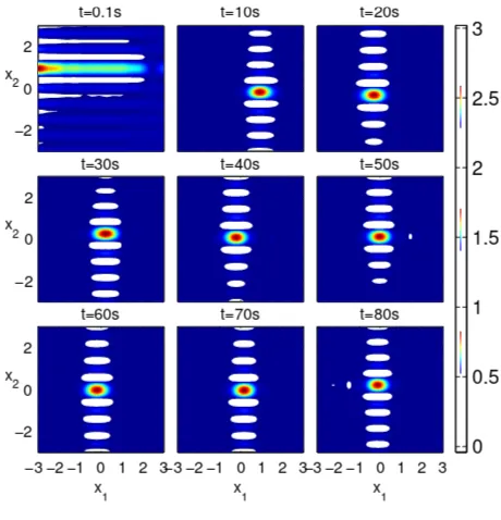
Fig. 4. Evolution of pdf at 10s intervals

forx1, and forx2. Fig. 4 shows the evolution of approximate

probability density function at 10s intervals. At t=0s, the pdf is uniform overΩ andE(x1) =0 andE(x2) =0, while

the true states are:x1(0) =−1 andx2(0) =1. As the pdf at

t=0.1s shown in Fig. 4,E(x1)andE(x2)converge to the true

[image:6.612.65.301.251.447.2] [image:6.612.320.550.289.528.2]

(7)

#4 IMU Sensors

x

y θ

[image:7.612.321.549.48.230.2]

(ax, ay)

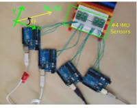
Fig. 5. Four IMU sensor configuration, wherexandyaxes are indicated.

be very careful in using the pdf integration over a subsection ofΩ. There will be some resolution limit in terms of the size of subsection area overΩ to calculate the probability.

C. Pointing estimation

Four inertial measurement unit (IMU) sensors are con-nected and kept stationary while they measure the accelera-tions, as shown in Fig. 5. In order to use the sensor measure-ments for a nonlinear estimation problem, a virtual pointing platform, where four sensors are attached, is assumed and its dynamics are given by

dθ=dβ,

yi_k=tan(θi k) +vik,

whereyi_kis thek-th measurement of thei-th sensor,Q=0.05,

Rfor each sensor is 0.618, 0.645, 0.404, 0.146, respectively, Ω= [−85◦,85◦], and the virtual sensor providing the mea-surement is constructed using the accelerometers as follows:

yi

k=aiy/aix, where aix and aiy are x and y directional accel-eration measurements respectively, from i-th IMU sensor. Ideally, if the platform is in the perfectly perpendicular to the gravitational acceleration, ai_x and ai_y are equal to zero. It is more likely that the surface is slightly tilted from the horizontal and both accelerations are affected by noise. Hence, the measurement provided by the virtual sensor, yi_k, would have very strong noise effects as shown in Fig. 6. All dots in Fig. 6 are the measurements at each instance, where each colour represents the measurement from each sensor. The measurements are available from around 5s, the true angle is zero and the estimated is indicated by the blue solid line, where the number of basis functions for the filter is 64. As shown by the measurements, the estimate ofθ is a lot better than the individual measurements and it is also better than a direct average of the four sensor outputs (not indicated).

V. CONCLUSIONS& FUTUREWORKS

Nonlinear projection filter was presented in the late 90’s and the computational complexity was the main obstacle for any practical implementations of the filter. Current increasing computational power and parallel architectures allow the practical application of the exact nonlinear filter. Several ways to improve the computation of the filter are presented based on Monte-Carlo integration and the usage of multiple parallel sensors. The performance of the proposed methods are demonstrated by two numerical examples and one exper-imental example. Future works will include: 1) applying the

0 5 10 15 20 25 30 35 40

−80 −60 −40 −20 0 20 40 60 80

time [s]

angle [degrees]

estimate true

Fig. 6. Pointing angle (θ) estimation, where all dots are the measurements.

filter for indoor navigation problem, whose state dimension could be up to twelve; 2) real-time re-positioning algorithm for the sampling space, Ω, while the states are progressed; and 3) implement the algorithms in GPU or FPGA.

ACKNOWLEDGEMENT

This research is supported by School of Mechanical En-gineering, University of Leeds, Leeds, UK.

REFERENCES

[1] R. E. Kalman, “A New Approach to Linear Filtering and Prediction Problems,”Transactions of the ASME Journal of Basic Engineering, no. 82 (Series D), pp. 35–45, 1960.

[2] M. S. Grewal and A. P. Andrews, “Applications of Kalman Filtering in Aerospace 1960 to the Present [Historical Perspectives],”Control Systems, IEEE, vol. 30, pp. 69–78, June 2010.

[3] E. J. Lefferts, F. L. Markley, and M. D. Shuster, “Kalman filtering for spacecraft attitude estimation,”Journal of Guidance, Control, and Dynamics, vol. 5, pp. 417–429, September-October 1982.

[4] S. J. Julier and J. K. Uhlmann, “Unscented filtering and nonlinear estimation,”Proceedings of the IEEE, vol. 92, pp. 401–422, Mar. 2004. [5] E. Wan and R. Van Der Merwe, “The unscented Kalman filter for nonlinear estimation,” in Adaptive Systems for Signal Processing, Communications, and Control Symposium 2000. AS-SPCC. The IEEE 2000, pp. 153–158, IEEE, Aug. 2000.

[6] M. S. Arulampalam, S. Maskell, N. Gordon, and T. Clapp, “A tutorial on particle filters for online nonlinear/non-Gaussian Bayesian tracking,”Signal Processing, IEEE Transactions on, vol. 50, pp. 174– 188, Feb. 2002.

[7] N. G. Van Kampen,Stochastic Processes in Physics and Chemistry, Third Edition (North-Holland Personal Library). North Holland, 3 ed., May 2007.

[8] R. Beard, J. Kenney, J. Gunther, J. Lawton, and W. Stirling, “Nonlin-ear Projection Filter Based on Galerkin Approximation,”Journal of Guidance, Control, and Dynamics, vol. 22, pp. 258–266, Mar. 1999. [9] G. Qian, K. Shafique, and P. Wang, “Fusion of nonlinear motion

dynamics using fokker-planck equation and projection filter,” in In-formation Fusion (FUSION), 2014 17th International Conference on, pp. 1–7, July 2014.

[10] NVIDIA, “CUDA parallel computing platform,” Mar. 2015. [11] L. Meirovitch,Analytical Methods in Vibrations. Macmillan

Publish-ing Co., Inc., 1967.

[12] X. Chen, Q. Dai, and C. Li, “A fast algorithm for computing multidimensional DCT on certain small sizes,” Signal Processing, IEEE Transactions on, vol. 51, pp. 213–220, Jan. 2003.

[image:7.612.127.227.49.128.2]