New pathways for improved quantification of energy-dispersive X-ray spectra of semiconductors with multiple X-ray lines from thin foils investigated in transmission electron microscopy

This is a repository copy of New pathways for improved quantification of energy-dispersive X-ray spectra of semiconductors with multiple X-ray lines from thin foils investigated in transmission electron microscopy.

White Rose Research Online URL for this paper: http://eprints.whiterose.ac.uk/91474/

Version: Accepted Version

Article:

Parri, M.C., Qiu, Y. and Walther, T. (2015) New pathways for improved quantification of energy-dispersive X-ray spectra of semiconductors with multiple X-ray lines from thin foils investigated in transmission electron microscopy. Journal of Microscopy, 260 (3). pp. 427-441. ISSN 1365-2818

https://doi.org/10.1111/jmi.12345

This is the peer reviewed version of the following article: PARRI, M.C., QIU, Y. and WALTHER, T. (2015), New pathways for improved quantification of energy-dispersive X-ray spectra of semiconductors with multiple X-ray lines from thin foils investigated in transmission electron microscopy. Journal of Microscopy, 260: 427–441. doi:

10.1111/jmi.12345, which has been published in final form at

https://dx.doi.org/10.1111/jmi.12345. This article may be used for non-commercial purposes in accordance with Wiley Terms and Conditions for Self-Archiving (http://olabout.wiley.com/WileyCDA/Section/id-820227.html)

[email protected] https://eprints.whiterose.ac.uk/ Reuse

Unless indicated otherwise, fulltext items are protected by copyright with all rights reserved. The copyright exception in section 29 of the Copyright, Designs and Patents Act 1988 allows the making of a single copy solely for the purpose of non-commercial research or private study within the limits of fair dealing. The publisher or other rights-holder may allow further reproduction and re-use of this version - refer to the White Rose Research Online record for this item. Where records identify the publisher as the copyright holder, users can verify any specific terms of use on the publisher’s website.

Takedown

If you consider content in White Rose Research Online to be in breach of UK law, please notify us by

This is the peer reviewed version of the following article  

New pathways for improved quantification of energy-dispersive X-ray

spectra of semiconductors with multiple X-ray lines from thin foils

investigated in transmission electron microscopy

which  has  been  published  in  final  form  at 

http://onlinelibrary.wiley.com/doi/10.1111/jmi.12345/abstract  

This article may be used for non commercial purposes in accordance with Wiley Terms and 

Conditions for Self Archiving.

New pathways for improved quantification of energy-dispersive X-ray

spectra of semiconductors with multiple X-ray lines from thin foils

investigated in transmission electron microscopy

M.C. Parri1, Y. Qiu1,2 and T. Walther1,3

1

Department of Electronic & Electrical Engineering, University of Sheffield, Mappin Street,

Sheffield S1 3JD, UK

2

now at: IMEC, Kapeldreef 75, B-3001 Leuven, Belgium

3

corresponding author: email: [email protected],

telephone: +44 114 222 5891,

fax: +44 114 222 5143

Abstract: Theoretical approaches to quantify the chemical composition of bulk and thin layer

specimens using energy-dispersive X-ray spectroscopy in a transmission electron microscope

are compared to experiments investigating (In)GaAs and Si(Ge) semiconductors. Absorption

correctors can be improved by varying the take-off angle to determine the depth of features

within the foil or the samples thickness, or by definition of effective k-factors that can be

obtained from plots of k-factors vs. foil thickness or, preferably, vs. the K/L intensity ratio for

a suitable element. The latter procedure yields plots of self-consistent absorption corrections

that can be used to determine the chemical composition, iteratively for SiGe using a set of

calibration curves or directly from a single calibration curve for InGaAs, for single X-ray

Keywords: energy-dispersive X-ray spectroscopy, analytical transmission electron

microscopy, quantification, k-factors

Introduction

The basic principles of energy-dispersive X-ray spectroscopy (EDXS) in a transmission

electron microscope (TEM) are well understood: by measuring the X-ray output of a material

using a semiconductor detector it is often possible to determine the chemical composition to a

good degree of accuracy. In very thin samples where X-ray absorption is negligible,

quantification is hampered by two effects: the small numbers of X-rays produced in very thin

foils mean that statistical errors will be high due to shot noise, and contributions from

surfaces in the form of contamination or surface oxide layers (cf. Walther and Humphreys

1997) can be large relative to ‘bulk’ contributions from inside the thin foil specimens and

cause systematic errors. Both effects could be reduced if thicker specimens were analysed,

and in transmission electron microscopes operated at intermediate voltages (200-300kV)

specimens of up to 1 m in thickness may be sufficiently electron transparent and can

therefore be studied.

One of the primary difficulties then is correcting for absorption and fluorescence within the

sample. The main parameters influencing absorption are chemical composition, density and

thickness of the material that the X-ray travels through, i.e. mass-thickness of the sample, and

take-off angle (Goldstein and Williams, 1981). Commercially available methods for

determining the chemical composition require the sample thickness and density for

approximate absorption correction, however calculating the thickness of the material

alone if several characteristic X-ray lines are present and the detector response function as

well as the take-off angle were precisely known. This report seeks to expand on that idea and

thus constitutes an alternative approach to the zeta-factor method of quantification where the

specimen’s chemistry and thickness can be iteratively determined if both mass absorption

coefficients and the absolute electron dose employed are precisely known (Watanabe et al.

1996).

The absorption correction in the original Cliff-Lorimer ratio (Cliff & Lorimer, 1975)

approach requires certain approximations: homogeneity along both the electron beam and

X-ray paths and that the density and thickness of the sample are known a-priori.

The assumption of homogeneity along the electron beam and X-ray directions implies that

minor local changes (such as due to stacking faults, impurities or the difference in chemistry

between top and bottom parts of the foil) can be ignored. The result of this is that the quantity

of X-rays produced and the number absorbed can be considered directly proportional to the

volume and composition of the sample (given that the beam energy is sufficiently high so that

the stopping power of the electrons does not vary significantly along the sample). A thicker

material will produce more X-rays, and hence, knowledge of the sample’s thickness is

necessary to accurately estimate the number of X-rays initially produced. The density of a

material has a correlation with the extent of absorption. Both of these factors have strong

effects on correct quantification.

The effect of absorption is to decrease the X-ray intensity exponentially according to the

following equation:

where I and I0 are the detected and generated X-ray intensities, respectively, t* is the

thickness of material the X-rays have travelled through and is the attenuation wavelength,

which is a particular value depending on the energy of the X-ray and the material of the

sample. The thickness t* is generally given by

t* = t/sin =t cosec (2),

where t is the vertical thickness of material between the origin of the X-ray and the sample

surface and is the take-off angle. Division by sin (or multiplication bycosec ) describes

the increase in path length within the material X-rays have to travel through towards the

detector placed under take-off angle , and smaller take-off angle means stronger absorption

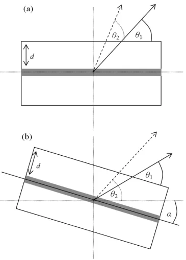
and fewer X-rays. It is worth noting that tilting the specimen by an angle , as sketched in

figure 2, increases the apparent specimen thickness by a factor of 1/cosa, creating

correspondingly more X-rays and also changes the take-off angle, leading to decreased

absorption if tilted towards but increased absorption if tilted away from the detector, and both

angles need to considered for accurate quantification.

The number of X-rays detected from element j in a sample of thickness t is given by

   (3)

where NA is Avogadro’s constant, Aj the atomic weight of element j (in g/mol), i the probe

current, e the electron charge, the density, cj the weight fraction, j the ionisation

cross-section, j the fluorescence yield, fj the line partitioning fraction (for K, L, M lines), aj the

absorption factor, ej the detection efficiency of line j and  the measurement time. Cliff and

Lorimer (1975) developed the basic thin film quantification approach by defining a factor kij

for two lines i,j as the ratio

 

so that without absorption (i.e. for ) one simply obtains

(5).

The weight fraction is then given by

(6)

and the atomic fraction by

(7).

For a multinary system of n elements rather than a binary system, where x1+x2+x3+…=1, and

with absorption, the Cliff-Lorimer method yields for atomic concentrations:

where n is an index running over all elements. The method requires that the k-factor be

defined relative to a standard. In this report, that standard is SiK, which is the most common

reference line. For shorthand we continue to write kj if we refer to kj,SiK.

The k-factor and the absorption correction are intractably linked, as only their product,

later-on called k*, can be measured in an experiment. This is a significant problem, since the

absorption and fluorescence correction will change depending on the thickness of the material

while the k-factor would not. A method for calculating an effective k-factor including X-ray

In the following, we describe three approaches for obtaining additional quantitative

information from X-ray spectra. Method 1 explores the consequences of specific

inhomogeneity: when there is a discrete structure (e.g., a precipitate or a region of very high

concentration of a certain element) embedded within the matrix of another composition then

changing the take-off angle can yield information on the depth of the feature within the foil.

This would be useful primarily for enhanced compositional analysis of embedded quantum

structures, such as quantum wires (Cui, Robertson, Robinson, Andrei, Thompson, Botton,

2009) or nanoparticles (Tsen, Crozier, Liu, 2003; Zak, Laval, Dluzewski, Kret, Yam,

Bouchier, Fossard, 2009). Method 2 attempts to calculate the thickness of a sample by

comparing the X-ray output from several related lines, e.g. K/L intensity ratios, thereby

permitting more quantitative analysis without needing to resort to other methods or rely on

simulations. This has been suggested before (Morris, Ball, Statham, 1979; Horita, Ichitani,

Sano, Nemoto, 1989) and would be most useful in samples with soft X-rays (Banchet,

Michel, Jallot, Laurent-Maquin, Balossier, 2003; Ivetic, Nikolic, Parakevopulos, Pavlidou,

Zorba, Nikolic, Ristic, 2008; West, Thomson, 2009; Laszcz, Czerwinski, Ratajcak, Szerling,

Phillipp, van Aken, Katcki, 2010) or where, as in certain cases of medical samples (Kirk,

Gates, Provance, Lee, 1997), an accurate knowledge of the thickness is critical for

quantification of thicker samples where absorption cannot be neglected. Method 3 describes

an aspect of how knowledge of the sample thickness or, preferably the K/L intensity ratio of a

heavier element, can permit more accurate quantification, similar to a procedure described

before (Horita, Ichitani, Sano, Nemoto, 1986; Horita, Sano, Nemoto, 1987 & 1991). As

examples, semiconductors of technological importance, such as Si(Ge) and (In)GaAs have

Experimental

All the experimental data presented here was gathered with a JEOL 2010F field-emission

transmission electron microscope (TEM) operated at 197kV, equipped with an URP

pole-piece with 2mm pole-pole-piece gap, and a Si:Li detector with 25° nominal take-off-angle,

ultrathin polymer window, Oxford Instruments ISIS 300 software, specimen tilt range

approximately -10° to +25°. Specimens investigated included:

i. GaAs wedge specimens, cleaved and viewed along <100> zone axis,

ii. InGaAs plan-view specimens, studied near <001> zone axis,

iii. InGaAs/GaAs cross-sections studied near <110> zone axis, all polished and argon ion

milled for perforation,

iv. SiGe/Si: as under iii. above

For comparing experimental and simulated data on absolute scales, as in Figures 1, 5, 8 and

9, the efficiency of our X-ray detector has been calculated with the DTSA-II code (Ritchie,

2009) and the resulting estimated detector efficiencies are listed in Table 1 for the relevant

X-ray lines considered.

Monte Carlo simulations

Four Monte Carlo programs were used to provide simulated data for comparison with

experimental results. These four were NISTMonte (Ritchie, 2005), CASINO (Hovington,

Drouin & Gauvin, 1997), Hurricane (Rickerby & Thiot, 1994) and EDAX Electron Flight

Simulator (EEFS) (Smallworld, 2012). EEFS does not apply relativistic corrections to the

scattering and ionisation cross-sections, and as such would likely give incorrect results for the

cancel out. EEFS only allows a maximum thickness of 3 m to be simulated, hence its graph

is truncated. All simulations were carried out for 1 million electron trajectories at 200keV and

assumed a detector efficiency of unity, while Table 1 suggests a ratio of eAsK/eAsL=1.16 in the

experiment.

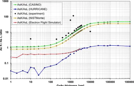
Figure 1 compares the simulated and experimental results of the AsK/AsL line intensity ratio

from a homogenous GaAs 90º wedge sample tilted very slightly off a [100] zone axis

orientation, on a double-log plot so an upwards shift of 16% of the experimental data will be

irrelevant. Experimental thicknesses were measured as twice the distance from the edge,

which is difficult to assess for very large thicknesses where the specimen appears pitch-black

in bright-field TEM mode and the magnification has to be reduced far enough so the edge can

actually be seen (while LOW MAG mode with the objective lens switched off has to be

avoided for EDXS as high energy electrons could directly hit the detector). All curves have a

similar form, with an inflection point around a thickness of ~2 m, indicating the absorption is

modelled with similar attenuation lengths in all of them. It is clear that the results from

NISTMonte and CASINO match the experimental much more closely than HURRICANE or

EEFS that are lower by factors between ~4x and ~30x (Walther, 2010a), which must be due

to incorrect ionisation cross-sections and/or fluorescence yields in the latter codes (only their

product enters in equation 3). Despite some outliers in experimental measurements

(presumably due to the difficulty in assessing very large thicknesses in experiments), we

conclude that if one wants to model X-ray absorption, one can either use tabulated values for

mass attenuation coefficients, e.g. from NIST (Hubbell and Seltzer 1996), or Monte Carlo

codes like NISTMonte or CASINO. We have chosen the latter to get a direct output of

intensities vs. specimen thickness for alloys not listed in these tables without having to

Figure 1 is thus to show that ionisation cross-sections (determining the height of the curves),

and thus also corresponding thin film k-factors, are less well predicted than X-ray absorption

Method 1: calculation of depths of features embedded within specimens from range of

specimen tilts

If there is a local structure or high concentration of a material embedded within a matrix of

another material, the assumption of the Cliff-Lorimer approach that the X-rays originate

equally from all points within the beam interaction volume is not valid.

It has been shown (Walther, 2008) that the intensity of detected X-rays, I, can be expressed

analytically as a function of generated intensity, Io, by:

exp (9)

where D = d cosec is the length of material the X-rays have effectively travelled through to

reach the detector, as sketched in Figure 2a, and is the attenuation wavelength, a constant

for a given X-ray energy in a specific material. For an infinitely thin layer imaged at depth d

the electron beam transverses perpendicularly, this can be algebraically reduced to

ln

cosec cosec

(10a)

Assuming that the feature has a well defined depth within the foil and that its self-absorption

can be neglected, this equation would permit the calculation of the depth of the X-ray source,

Unfortunately, most microscopes do not allow for the detector to be moved to vary the

take-off angle. This can be substituted by tilting the specimen when a change in take-take-off angle is

required, as sketched in Figure 2b. However, doing so noticeably increases the effective

specimen thickness in projection and thus the interaction volume, by a factor of 1/cos . The

detected intensity must be multiplied by the cosine of the specimen tilt angle to convert the

experimental intensity to what would be expected from a flat horizontal sample and a

modelled tilted detector. In the following, this correction, which for tilts from = 10° to +25°

range amounts to relative corrections of up to 1/cos 25° 1=10.3%, has been applied

throughout to all experiments and simulations with tilted specimens, i.e. equation (10a) for

detector tilt effectively turns into equation (10b) for specimen tilt:

ln cos cos

cosec cosec

(10b)

Note that the cosine factors are due to changes in projected thickness (when tilting the

specimen) while the cosec factors are due to the change in take-off angle. The angular

correction to the numerator in equation (10b) depends strongly on the intensity ratio I1/I2 and

is maximal if this intensity ratio approaches unity, as the logarithm function then has the

largest gradient (note I1>I2 for 1 > 2 guarantees the logarithm is only ever evaluated

for values >1). A major experimental issue was that, despite experiments close to the

eucentric height, any large specimen tilts led to some lateral displacements which we tried to

compensate by careful lateral movement of the specimen holder by the piezo stage to retain

the weak contrast features visible in plan-view geometry in order to ensure that the same

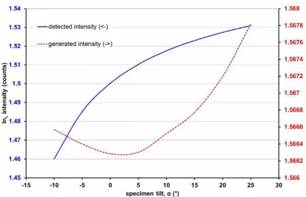
Figure 3 illustrates the simulated curve expected from a thin layer with changing take-off

angle for a 1nm thick InAs layer embedded 50nm deep within a GaAs sample 120nm thick.

The form of the exponential curve of ‘detected intensity’ describes the X-ray intensity

including absorption and is characteristic for the tilted sample geometry, regardless of

material. The ‘generated intensity’ curve is much flatter (note the enlarged scale of the right

vertical axis) and demonstrates that the geometrical correction for tilt (multiplication by cos

) is not entirely effective, as a perfect correction would result in no change in X-ray

generation with changing tilt at all. The change observed is due to the electrons in the beam

losing energy as they travel through more material and therefore experiencing an increased

stopping power, which in turn increases X-ray generation. The change in the ‘generated

intensity’ is very small (<1%) in comparison to the ‘detected intensity’.

Table 2 contains the results from applying equation (10b) to the simulated data of Figure 3. It

is clear that the numerical evaluation is working well for low tilts but becomes increasingly

incorrect with greater take-off angles. The beam straggling effect means that any fit

calculated from two relatively high tilts should be ignored: precisely what tilt range can be

used will be dependent on the X-ray in question and the thickness and composition of the

capping layer and the accuracy required. For the tilt range -10°< <20° the average value and

the standard deviation from the output of these simulations is 51.7±1.5nm, which is 2.3±3.0%

higher than the input value of 50.5nm (for all values the result would be 52.5±3.1nm). It is

worth noting that the input data has an expected standard deviation of less than 0.02% in

these simulations, based on 3×107 X-ray events simulated, implying that even small

systematic changes in the measured intensity would result in much larger errors in the

evaluation. Assuming equal errors from Poisson counting statistics and background

comparable accuracy in any experiment, which would be impractical for most experiments.

However, such high count rates would only be necessary in a system that has such a small

quantity of the material of interest (here, a 1nm InAs embedded in 50nm GaAs means an

effective indium concentration of ~1at%): a greater amount of indium would see a lower

requirement for counts.

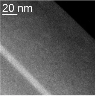
This method was applied to an 8nm thick In0.24Ga0.76As layer embedded 95nm deep within

GaAs. Layer thickness, position and composition were confirmed by analysis of a

cross-sectional sample, as shown in Figure 4.

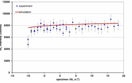
Figure 5 shows the InL intensity detected from this sample at different experimental tilts from

-10º to +18º. For large tilts away from the detector ( ≤–11º) the holder shielded X-rays

emission completely, which is not taken into account in the simulation. This shadowing effect

explains the pronounced fall-off in counts for such tilts. It is clear that while the statistics are

poor, as only ~1% of the sample volume is occupied by In atoms contributing to the signal,

the overall trend of the curve matches the simulations.

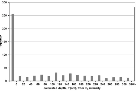
Looking at Figure 6, which tries to recover the layer depth numerically, it is however clear

that no legible answer is available. This appears to be a consequence of the data’s poor

statistics, which is itself a result of attempting to acquire a large number of spectra (i.e.

intensities for the maximum number of tilts) for a weak signal.

However, another method can also be applied to the same data: by simulating the 8nm

In0.24Ga0.76As with different GaAs overlayer thicknesses it would be theoretically possible to

what depth the simulations imply to be the correct value. This closest match can be found by

plotting the sum of squares against simulated overlayer thickness, where the minimum would

be the most likely, and hopefully correct, answer. Since the experimental and simulated data

are on different absolute scales, it is necessary to normalise the simulated data to the same

scale as the experimental. As no experimental data point would be ideal for normalising with

respect to, the normalisation has been carried out with respect to all experimental data points

individually. Not every curve possesses a minimum: these would be the result of the

experimental data point being so far from the expected curve that the simulations either

continually move away or converge above some unphysical overlayer thickness (in this case,

>200nm). Further, some smoothing was attempted by averaging over two (‘pairs’) or three

(‘triplets’) data points.

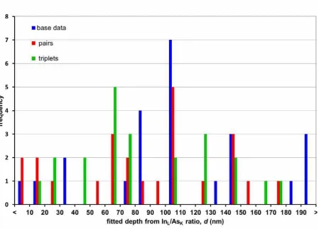
Attempting this method using the InL intensities alone does not give reasonable answers:

most curves give a result larger than 200nm. However, applying the same procedure to the

measured InL/AsK ratio does give meaningful results, as seen in Figure 7. The values

calculated here are not only physically reasonable but agree with the true depth value, albeit

with large error bars. The difference in behaviour between the InL and InL/AsK results could

be due to the large scatter from statistics being counteracted by the normalisation by AsK.

In summary, a fairly typical sample was examined using equation (10b) and it was found that

inferior statistics could produce so much scatter as to invalidate the approach. However,

comparing experimental intensity ratios to simulated results does seem to give reasonable

answers. While such a comparison to simulations is time consuming to carry out it does show

some promise by extracting meaningful results from experiments with even rather poor

a specimen foil can be determined from comparative measurements at different tilts, then

absorption corrections for X-rays can be improved and a higher reliability of any

compositional estimate may be obtained. In the above example, the depth of the flat InAs

layer beneath the surface of a GaAs specimen could be predicted with about ±10% relative

accuracy, corresponding to ~10nm, as given by the mean peak position error of fitting a

distribution to the histogram in Figure 7, however, the width of the distribution as given by

the random mean square error is much larger (~50nm), and more complicated shapes of

buried features could have a profound effect on the variation of an X-ray intensity ratio with

specimen tilt. In conclusion, we propose to use experimental X-ray intensity ratios and

perform a multiple least-squares fit to all possible combinations of tilt angles to determine the

most likely depth of a feature in the foil from equation (10b). This can then be used to

improve standard X-ray absorption corrections, although the scatter of the resulting numerical

depth values obtained may remain rather large due to limited signal-to-noise ratios in typical

X-ray spectra.

Method 2: determination of sample thickness from K/L intensity ratios

The degree of absorption for a particular X-ray line is dependent on three factors: the density

and composition of the material travelled through, the amount of material to travel through,

and the energy of the X-ray. By analysing different X-ray lines (i.e. those with different

energies) for the same element from the sample in the same geometry, it is possible to deduce

the extent of absorption. By then studying areas of different thicknesses of the sample while

still analysing the same two X-ray lines, it should be possible to calculate the effect that

thickness has on absorption. If the ratio of these two X-ray lines are plotted for many

composition and density who exhibit the same set of X-ray lines (amongst possibly many

others) more quantitatively by deriving their sample thickness affecting absorption by

interpolating between points on this calibration curve.

Based on this idea, different ways of parameterisation of absorption have been tested over the

decades: Morris, Ball and Statham (1980) plotted Cu/Al compositional ratios vs. mass

absorption coefficients where the latter had to be iteratively fitted to Cu K/L line ratios.

Horita, Sano and Nemoto (1986) plotted an effective k-factor vs. absolute specimen thickness

measured in nanometres, which they showed later is rather difficult to experimentally

measure reliably (Horita et al., 1989). Horita, Sano and Nemoto (1987) and van Cappellen

(1990) also plotted atomic ratios vs. the measured total intensity of a specific (hard) X-ray

line to perform an absorption correction, however, absolute X-ray counts will depend on the

total beam intensity and thus will only be comparable for a series of measurements in one

specific microscope under exactly the same conditions. All these parameterisations need

series of measurements to extrapolate the effect of absorption down to zero thickness to get

the Cliff-Lorimer k-factor appropriate for thin films.

In the following we show that simulations suggest almost linear changes of K/L intensity

ratios with specimen thickness over ranges typical of foils examined in transmission

geometry, however, numerical results from different simulation programs differ by so much

that the endpoints for reliable fits must be obtained from experimental measurements. In

particular, the assumption of simple analytical models that the average X-ray emission event

occurs in the middle of the foil neglects not only any fluorescence but also the strong

non-linearity of the absorption of softer X-rays, which means that the intensity from the middle of

Therefore, substituting tabulated X-ray absorption lengths into an exponential absorption

curve assuming half the foil thickness will be inappropriate, and we again used Monte Carlo

simulations to predict X-ray intensities. For small thicknesses, an alternative would have been

to perform a simple line integral of an absorption-modified X-ray intensity assuming uniform

ionisation along the electron path, however, neglecting beam straggling and stopping power

variations is only permissible up to ~100nm for 200kV electrons, while our simulations cover

a range up to 2 m thickness and experimental data are for lamellae up to ~1 m thick..

Figure 8 compares results for GaAs using NISTMonte and CASINO simulations, with same

detector sensitivities, to experiments. Up to 2 m thickness the simulated plots are nearly

linear. As demonstrated in Figure 1, this pattern does not hold beyond a certain thickness but

should be valid for typical specimen thicknesses in transmission electron microscopy. The

difference between the two programs is consistent with that of Figure 1. The experimental

data was gathered from four areas of a lamella that had been milled by a focused ion beam

(FIB) to the specified thicknesses. It seems clear that the experimental data deviate

significantly from the simulated results, in that the CASINO Ga K/L ratio agrees with the

experimental data better than NISTMonte, while the reverse is true for the As K/L ratio. This

is troublesome, as it implies that neither program can be relied upon to give results that are

directly comparable to experiment, even if detector sensitivities are taking into account. More

experimental data points at different thicknesses would aid the choice of the best fitting

simulated curve by simply improving the reliability of the linear least-squares fit.

Figure 9 shows similar simulations for a SiGe sample (Ge K/L only, as Si does not have an

easily quantifiable L-line).

Table 4 compares the linear least-squares regression of the data in Figure 9. It can be seen

that CASINO has higher scatter and lower R2, in addition to beginning higher and increasing

slightly faster. Recently determined experimental results (Qiu et al., 2013) indicate that the

correct value for the intercept would be 1.30±0.05, which agrees with CASINO but disagrees

with NISTMonte.

The major conclusion is that the K/L ratio appears to remain linear over useful ranges of

TEM specimen thicknesses. The consequence of this is that very few data points would be

needed to construct such a plot for any material, as it is simply a matter of linearly

extrapolating from the available points. In effect, the number of points needed is more

strongly dependent on their error bars than any other factor, and in principle a K/L intensity

ratio for a very thin sample (t0nm) and another values for a thick sample area of

well-known thickness (e.g. 1 m) would be sufficient. The experimental problem will be to obtain

X-ray measurements for a precisely known large thickness, say ~1 m with an error of less

than 20nm, which could serve as upper calibration point. Then, in related samples of similar

density and/or composition, a simple K/L intensity ratio extraction would allow a quick

thickness estimate and hence a more reliable absorption correction using standard software.

Method 3: Improved accuracy of chemical composition measurement by sets of thickness-dependent k-factors

The ‘k-factor’ of the Cliff-Lorimer method is defined relative to another X-ray line.

Generally, this line is SiK though FeK is sometimes used. As such, in the specific case of

Si1−xGex, kSiK = 1 by definition, aSiK= 1 by defining the absorption relative to that of SiK for

simplicity and x = xGe = 1–xSi, which permits reducing the calculation of the effective k

(11)

where, again, I describes the measured intensities (now in thicker samples) and A the atomic

weights. This k* factor is the product of the classical thin film k-factor from equation (4) and

the absorption correction factor a from equation (3).

We can only separate the k-factor and absorption terms for t=0 where absorption is negligible

(a≈1), and in practice k-factors have often been measured for samples assumed to be

sufficiently thin to assume a = 1, usually without this having been proven. This can be better

achieved by calculating values of k* for a number of data points with decreasing sample

thickness, and extrapolating to zero thickness, as the k* values at zero thickness would have

an absorption of unity (Horita, McCartney and Weiss, 1992; Walther, 2010b). k* would then

be a thickness dependent k-factor which would permit more accurate quantification of

homogenous or near homogenous samples of known thickness. If a reliable thickness value is

not available and the estimate is wrong, then quantification results from K- and L-lines from

the same element (here GeK and GeL) would differ. This may be improved, rather than by

averaging, by choosing a thickness value consistent with the experimentally measured K/L

ratio (see method 2 and Morris, Ball, Statham, 1980; Horita, Ichitani, Sano, Nemoto, 1989).

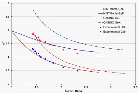
Figure 10 shows simulated and experimental results for Si0.54Ge0.46 (Qiu et al., 2013). It is

clear that while the general form of the trend is consistent between simulation programs and

experimental results, the curvature and termination points of the curves differ considerably.

Of the two programs, CASINO appears to be closer to experiment in this case. Extrapolating

using a second order polynomial yields k* at t=0 for GeK of ± and GeL of

2.004±_0.0720.075, whereas Oxford Instruments’ ISIS software gives values of 1.609 and 1.654,

Figure 11 shows plots of k*-factors simulated by CASINO for both Ge lines (L at the top, K

at the bottom) for germanium concentrations of x=0.1, 0.3, 0.5, 0.7 and 0.9. While the latter

two sets for x=0.7 and 0.9 almost overlap, sets for low Ge concentrations yield different

calibration curves for k* vs Ge K/L intensity ratio. As all curves are monotonic, do not cross

and are sorted so the ones for lowest Ge concentrations yield the largest k*-factors, it is

possible to iteratively determine x, and the result is independent of the starting curve used. If

for example, a 1050nm thick (!) Si0.8Ge0.2 specimen yields a Ge K/L ratio of 1.644 and one

looks this K/L value up in the calibration curves for x=0.1 [0.3] then the estimated k*GeL

factor would be 2.361 [1.699], which from the measured intensities would predict x=0.231

[0.178]. So, curves with a too low [high] reference value would predict too high [too low]

values for k* and thus also x. Hence, the problem is solely to find iteratively the correct

calibration curve, which is given by the one for a value xcal that best matches the value xout if

the corresponding k*-factor from this curve is used. This ensures self-consistency for

quantification using either Ge L or K lines. The precision is merely a matter how densely

sampled the calibration curves are. In our case, with an increment of only x=0.2, we by

interpolation get x=0.2050.027 from the Ge L quantification curves for x=0.1 and 0.3 (and a

very similar value for Ge K quantification). For x<0.1 one would need a few more curves for

lower reference compositions (x=0.02, 0.04 and 0.07 may suffice) as these are more widely

spaced for same x increments than for higher x values. For x>0.7 the calibration curves are

so similar that no iteration will be needed as it would not matter which one was used.

In the more general situation where silicon is not present, the k-factor of the second material

will not be equal to unity. However, a k-factor calculated relative to another element will

implicitly also be relative to whichever line that other k-factor was calculated with respect to,

K/L line ratios if the densities of the compounds the X-ray lines are measured from do not

change too much, but not if the latter were plotted as function of absolute thicknesses as in

Figure 12.

At the moment, there are no corrected k-factors for the GaK,L or AsK,L lines that would allow

them to be expressed relative to SiK. As such, the k* calculated in Figures 12 and 13 are with

respect to the AsK line, as this has the highest energy and therefore is the least absorbed.

Simulated results indicate that an appropriate fit against K/L ratio (cf. Figure 11 for SiGe)

would be at least second order polynomial. The results of a similar fit to Figure 12 are shown

for GaAs in the third column of Table 5, with the 10nm data point (which simulations

indicate is an outlier) either included or omitted, respectively: this would give values for k

-factors extrapolated to zero thickness. Values for these standard k-factors, taken from Oxford

Instruments ISIS software, are shown for comparison. Obviously, these are defined with

respect to SiK so the values shown here were calculated as kAB= kA,SiK / kB,SiK. Unfortunately,

while the GaK/AsK data are plausible and have sufficiently small relative errors to be useful,

the remaining lines either scatter too much or, as for AsL/AsK without the 10nm data point,

are unphysical. Figure 12 demonstrates that direct measurements of k-factors from thin

samples can show systematic artefacts (due to surface damage during preparation, oxidation

or irradiation damage), compared to an extrapolation from a series of measurements with

improved statistics at higher thicknesses.

Attempting this analysis with respect to AsK/AsL or GaK/GaL intensity ratios plotted vs. As

K/L line intensity ratio instead of absolute thickness gives the improved results shown in 

AsK/AsL. In these cases, it was not necessary to exclude any data points, as those which were

previously outliers now lie much closer to the expected curve, as seen in Figure 13. Here, the

R2 goodness of fit values are uniformly higher and all values are physically reasonable,

indicating that the resulting values are superior to those seen in Table 5. In theory, it would be

expected that the k*-factor value for an X-ray line plotted vs. AsK/AsL or GaK/GaL would be

identical if extrapolated to t=0: differences may be attributed to numerous factors such as

incorrect detector efficiencies or K/L intensity ratios extrapolated to t = 0. For the GaK line, k

-factors extrapolated from plots vs As K/L and Ga K/L agree to within 3%.

Experimentally, there are two different ways to determine k*: either by determining the

absolute sample thickness or indirectly via the K/L ratio. While absolute specimen

thicknesses are experimentally difficult to measure to high accuracy and would necessitate

independent data from other methods (such as electron energy-loss spectroscopy or

convergent beam diffraction if the specimen geometry were not known a-priori), choosing

K/L intensity ratios instead as the horizontal axis instead means we rely only on data from

X-ray spectra and so obtain an inherent self-calibration. The advantage of the K/L ratio method

thus is that the result is always self-consistent for the area being examined (since the same

data set is being used).

In analogy to equation (11), k*-factors for the In L-line in an InxGa1-xAs alloy can be defined

with respect to a Ga line as

(12)

or, with respect to an As line, as

(13).

Figure 14 finally plots CASINO simulations of k*InL,As for both As lines (top: AsL for

the values for different alloy concentrations move along EXACTLY THE SAME LINE as

the thickness is changed but all fall onto one universal curve for all values of x considered. If

the In content for InxGa1-xAs is changed, or if the thickness is changed, then absorption

affects also the As K/L ratio value and one would simply move along the SAME curve to a

DIFFERENT POINT. If we plotted k* InL,Ga for both Ga lines as function of Ga K/L ratio

instead, then the situation would be rather similar to the situation for Si1-xGex considered

before and we would need a set of calibration curves for different concentrations, which

could be solved iteratively.

The general validity of the above proposed approach of using a K/L ratio measurement from

an experimental X-ray spectrum for a self-consistent absorption correction has recently been

demonstrated for various In and Ga containing compound semiconductors (Walther and

Wang 2015), with an emphasis on InGaN where only the Ga K/L ratio can serve as thickness

reference. We could also show that this method is rather insensitive to variations in detector

sensitivities and so should be rather widely applicable.

Conclusion

Three methods describing more effective quantification of X-ray spectra in analytical TEM

have been presented. To summarise: plotting K/L ratio against sample thickness gives an

approximately linear curve for sample thicknesses ≤1µm, it may be possible to exploit the

geometric change induced by changing the take-off angle to determine the depth of a buried

thin layer (if it lies in a range where the absorption of the corresponding X-ray changes

noticeably), and refining the process for calculating effective k-factors based on an indirect

absorption correction resulting from consistent K/L quantification appears to be possible, as

ratios, ideally for an element whose concentration is fixed (as for As K/L in a pure arsenide

compound), is preferable to plots as function of absolute specimen thickness.

Acknowledgement

The authors would like to thank two very knowledgeable reviewers whose critical remarks

References

Banchet V., Michel J., Jallot E., Laurent-Maquin D. and Balossier G. (2003) Light elements

quantitative x-ray microanalysis of thin samples in STEM. Absorption correction using

EELS data. J. Phys. D: Appl. Phys.36, 1599-1604.

Cliff G. and Lorimer G.W. (1975) Quantitative analysis of thin specimens. J. Microscopy

103, 203-207.

Cui K., Robertson M.D., Robinson B.J., Andrei C.M., Thompson D.A. and Botton G.A.

(2009) Quantitative compositional analysis and strain study of InAs quantum wires

with InGaAlAs barrier layers. J. Appl. Phys.105, 094313.

Goldstein J.I. and Williams D.B. (1981) X-ray microanalysis of thin specimens, in: Proc.

Quantitative Microanalysis with High Spatial Resolution, Manchester (eds. G.W.

Lorimer, M.H. Jacobs and P. Doig), pp. 5-14. The Metals Society, London.

Horita Z., Sano T. and Nemoto M. (1986) An extrapolation method for the determination of

Cliff-Lorimer kAB factors at zero foil thickness. J. Microscopy-Oxford 143, 215 -231.

Horita Z., Ichitani K., Sano T. and Nemoto M. (1989) Applicability of the differential X-ray

absorption method to the determination of foil thickness and local composition in the

analytical electron microscope. Philos. Magazine A 59, 939-952.

Horita Z., Sano T. and Nemoto M. (1987) Simplification of X-ray absorption correction in

thin-sample quantitative microanalysis. Ultramicroscopy21, 271-276.

Horita Z., Sano T. and Nemoto M. (1991) A new form of the extrapolation method for

absorption correction in quantitative X-ray microanalysis with the analytical electron

Horita Z, McCartney, MR and Weiss JK (1992) Computer-assited extrapolation method for

absorption correction in quantitative X-ray microanalysis. Ultramicroscopy 45,

263-265.

Hovington P., Drouin D. and Gauvin R. (1997) CASINO: A new Monte Carlo code in C

language for electron beam interaction.1. Description of the program. Scanning 19,

1-14.

Hubell J.H. and Seltzer S.M. (1996) Tables of X-ray Mass Attenuation Coefficients and Mass

Energy-Absorption Coefficients from 1keV to 20MeV for Elements Z=1 to 92 and 48

Additional Substances of Dosimetric Interest, http://www.nist.gov/pml/data/xraycoef/

Kirk R.G., Gates M.E., Provance A.J. and Lee P. (1997) Quantitative X-ray images

calculated on the basis of mass and volume. Microsc. Microanal.3, 512-519.

Liew S.L., Walther T., Irsen S., Hopkinson M., Skolnick M.S. and Cullis A.G. (2007)

Investigating the capping of InAs quantum dots by InGaAs. Springer Proc. in Physics,

120, 259-262.

Morris P.L., Ball M.D. and Statham P.J. (1980) The correction of thin foil microanalysis data

for X-ray absorption effects. Proc. EMAG 1979 conference, Inst. Phys. Conf. Ser. No.

52, 413-416.

Qiu Y., Nguyen V.H., Dobbie A., Myronov M. and Walther T. (2013) Calibration of

thickness-dependent k-factors for germanium X-ray lines to improve energy-dispersive

X-ray spectroscopy of SiGe layers in analytical transmission electron microscopy. Proc.

18th Microsc. Semicond. Mater., Oxford. J. Phys. Conf. Ser.471, 012031.

Rickerby D.G. and Thiot J.F. (1994) X-ray microanalysis of thin-film layered specimens

containing light elements. Mikrochimica Acta114, 421-429.

Ritchie N.W.M. (2005) A new Monte Carlo application for complex sample geometries. Surf.

Ritchie N.W.M. (2009) Spectrum simulation in DTSA-II. Microsc. Microanal.125, 454-468.

SmallWorld. http://www.small-world.net/efs.htm [Online] 2012. [Cited: 27 November 2012.]

Tsen S.-C.Y., Crozier P.A. and Liu J. (2003) Lattice measurement and alloy compositions in

metal and bimetallic nanoparticles. Ultramicroscopy98, 63-72.

Van Cappellen, E. (1990) The parameterless correction method in X-ray microanalysis.

Microsc. Microanal. Microstruct. 1, 1-22.

Walther T. and Humphreys C.J. (1997) Quantification of the composition of silicon

germanium/ silicon structures by high-angle annular dark-field imaging. Proc. EMAG

1997, Cambridge. Inst. Phys. Conf. Ser.153, 303-306.

Walther T. (2008) A simple method to improve the quantification accuracy of

energy-dispersive X-ray microanalysis. Proc. EMAG 2007 conference, Glasgow (eds. R.T.

Baker, G. Möbus and P.D. Brown) J. Phys.: Conf. Ser.126, 012090.

Walther T. (2010a) Comparison of experimental and theoretical X-ray intensities from

(In)GaAs specimens investigated by energy-dispersive X-ray spectroscopy in a

transmission electron microscope. Proc. 16th MSM, Oxford (eds. T. Walther, P.D.

Nellist, J.L. Hutchison and A.G. Cullis) J. Phys.: Conf. Ser.209, 012029.

Walther T. (2010b) An improved approach to quantitative X-ray microanalysis in (S)TEM:

thickness dependent k-factors. Proc. EMAG 2009 conference, Sheffield (ed. R.T.

Baker) J. Phys.: Conf. Ser.241, 012016.

Walther T. and Wang X. (2015) Self-consistent method for quantifying indium content from

X-ray spectra of thick compound semiconductor specimens in a transmission electron

microscope. J. Microsc., in print, doi: 10.1111/jmi.12291

Watanabe M., Horita Z. and Nemoto M. (1996) Absorption correction and thickness

determination using the zeta factor in quantitative X-ray microanalysis.

Williams D.B and Carter C.B (1996) Transmission Electron Microscopy, Plenum Press, New

York.

Zak M., Laval J.-Y., Dluzewski P.A., Kret S., Yam V., Bouchier D. and Fossard F. (2009)

Influence of the Si cap layer on the SiGe islands morphology. Micron40,122-125.

Figures

Figure 1: Comparison of X-ray intensity ratios from simulation programs to experimental

Figure 2: Geometric diagram of system for different take-off angles: (a) principle and (b)

Figure 3: NISTMonte simulation results for InL line intensity from a 1nm InAs layer

embedded within a 120nm thick GaAs matrix at a depth of 50nm. Beam energy = 197keV,

take-off angle of 25°. ‘Generated intensity’ is plotted against the secondary vertical axis to

the right and refers to all X-rays produced in a tilted sample, multiplied by cos , while

‘detected intensity’ includes the absorption effect due to GaAs coverage and finite take-off

Figure 4: Cross-sectional annular dark-field (ADF) STEM image of 8nm thick In0.24Ga0.76As

Figure 5: InL line intensity from 8nm thick In0.24Ga0.76As layer embedded under 95nm of

GaAs. Simulation normalised with respect to experimental 0° tilt data point. = + 25°.

Simulation run in NISTMonte at beam energy 197keV with 106 electron histories, for an 8nm

Figure 6: Result of applying equation (10b) to the data of Figure 5. = 2525nm. Nominal d

is dtrue=99nm. Average of all values between 0nm and 500nm is dexp=200±132nm, where

Figure 7: Histogram of results from fitting InL/AsK simulations of varying overlayer

thicknesses to experimental data. Known correct value is d = 99nm. Average overall:

95.3±50.6nm, mean error of the mean: 6.0nm. Average for ‘base data’: 108.5±54.4nm, mean

error of the mean: 11.1nm. Average for ‘pairs’: 87.6±49.6nm, mean error of the mean:

Figure 8: Comparison of NISTMonte and CASINO simulations to experimental results of

Figure 9: NISTMonte and CASINO results of K/L line ratios for Si0.54Ge0.46. Beam energy =

Figure 10: Comparison of simulated and experimental k*(from equation 6) vs. specimen

thickness for Si0.54Ge0.46. Beam energy = 197keV, take-off angle of 25°.

Figure 11: k* factors simulated for Si1-xGex alloys of different Ge content x. CASINO, beam

Figure 12: k* for cleaved wedge specimen vs specimen thickness for GaAs. GaK/AsK is

plotted against the second vertical axis on the right. The error bars of the AsL/AsK 10nm point

were truncated for clarity as they extend from below zero to 54. Thickness was measured by

how far the beam was moved away from the wedge’s edge (thickness = twice distance from

Figure 14: k* factors simulated for InxGa1-xAs alloys of different In content x. CASINO,

Tables

X-ray line starting energy [keV] detector efficiency 

GaL 1.10 0.65

GeL 1.19 0.67

AsL 1.28 0.68

SiK 1.74 0.70

InL 3.29 0.73

GaK 9.24 0.77

GeK 9.88 0.78

AsK 10.53 0.79

InK 24.14 0.89

Table 1: Detector efficiencies of X-ray lines calculated by DTSA-II program (Ritchie, 2009).

2 (°)

-5 0 5 10 15 20 25

1(°) -10 50.12 50.08 50.32 50.32 50.68 50.88 51.44

-5 50.02 50.53 50.48 51.07 51.36 52.2

0 51.3 50.9 51.79 52.14 53.35

5 50.34 52.2 52.66 54.43

10 54.75 54.48 56.82

15 54.11 58.37

20 63.91

Table 2: Calculated depth values d (nm) from Figure 3 and Equation (10b). Simulation

run in NISTMonte (beam energy of 197keV, take-off angle of 25°, = +25°). The

intensity line ratio slope (x10-3) intercept R2

AsK/AsL (Experimental) 3.34±0.30 1.07±0.20 0.984

AsK/AsL (CASINO) 5.30±0.03 0.97±0.02 0.998

AsK/AsL (NISTMonte) 3.61±0.03 0.71±0.02 0.999

GaK/GaL (Experimental) 1.90±0.15 1.50±0.10 0.987

GaK/GaL (CASINO) 2.12±0.03 1.16±0.02 0.994

GaK/GaL (NISTMonte) 1.76±0.02 0.81±0.01 0.998

Table 3: Linear least-squares regression of data in Figure 8.

intensity line ratio slope (x10-3) intercept R2

GeK/GeL (CASINO) 0.897±0.010 1.400±0.007 0.9962

GeK/GeL (NISTMonte) 0.869±0.001 0.996±0.001 0.9998

Table 4: Linear least-squares regression of data in Figure 9.

X-ray line ISIS k-factor with

respect to AsK

from fig. 12, all data points

included

from fig. 12, the data point

at t=10nm excluded

k* (t->0) R2 of fit k* (t->0) R2 of fit

GaK 0.877 0.68±0.04 0.679 0.77±0.02 0.949

GaL 0.985 1.17±0.45 0.924 0.14±0.23 0.989

AsL 1.012 2.95±1.56 0.850 -0.83±0.51 0.992

ISIS k-factors with

respect to AsK

from fig. 13, against

AsK/AsL

from fig. 12, against

GaK/GaL

X-ray line k* (t->0) R2 of fit k* (t->0) R2 of fit

GaK 0.877 0.73(2)±0.00(6) 0.975 0.70(4)±0.00(4) 0.956

GaL 0.985 0.81±0.05 0.992 1.05±0.05 0.999

AsL 1.012 1 1 2.10±0.16 0.992

Table 6: Comparison of corrected k*-factors with respect to AsK. Intensity ratio at t = 0 taken