Andreas Zollmann
A Consistent and Efficient Estimator for the Data-Oriented Parsing Model
MoL-2004-02,received: May 2004
ILLC Scientific Publications
Series editor: Benedikt L¨owe
Master of Logic Thesis(MoL) Series, ISSN: 1387-1951
Institute for Logic, Language and Computation (ILLC) University of Amsterdam
Plantage Muidergracht 24 NL-1018 TV Amsterdam The Netherlands
Abstract
Given a sequence of samples from an unknown probability distribution, a statistical estimator aims at providing an approximate guess of the distribution by utilizing statistics from the samples. One desired property of an estimator is that its guess approaches the unknown distribution as the sample sequence grows large. Mathematically speaking, this property is calledconsistency.
This thesis presents the first (non-trivial) consistent estimator for the Data-Oriented Parsing (DOP) model. A consistency proof is given that addresses a gap in the current probabilistic grammar literature and can serve as the basis for consistency proofs for other estimators in statistical parsing. The thesis also expounds the computational and empirical superiority of the new estimator over the common DOP estimator DOP1: While achieving an exponential reduction in the number of fragments extracted from the treebank (and thus parsing time), the parsing accuracy improves over DOP1.
Acknowledgements
This thesis could never have been completed without the help of several people. At the very first I want to thank my advisor Khalil Sima’an, who has been absolutely terrific. He was the one who got me excited about statistical NLP in his course on probabilistic grammars, whose interactive atmosphere had that fascinating research smell. During the time of my thesis work, I spent scores of invaluable discussions in his office. Concerning style and legibility, he simply didn’t let me get away with anything. Looking back at my first draft of the DOP∗ chapter, that was more than necessary.
I’d also like to thank Detlef Prescher for his advice on the estimation theory chapter and for reading and commenting on the thesis. Many thanks to Nguyen Thuy Linh as well, who provided me with some very fundamental insights into Data-Oriented Parsing.
Contents
1 Introduction 5
1.1 Outline . . . 9
2 Background 10 2.1 Terminology . . . 11
2.2 Data-Oriented Parsing . . . 12
2.2.1 The General Framework . . . 13
2.2.2 The DOP1 Estimator . . . 14
2.2.3 DOP1 Is Inconsistent . . . 14
2.2.4 DOP1 Is Biased Towards Fragments of Large Parse Trees . 16 2.2.5 Other Existing DOP Estimators . . . 17
2.3 Probability Models and The Principle of Maximum-Likelihood Es-timation . . . 20
2.4 Held-Out Estimation . . . 22
3 Considerations about Bias and Consistency 25 3.1 Basic Notions . . . 25
3.1.1 Estimation . . . 25
3.1.2 Bias, Loss Function, and Consistency . . . 26
3.1.3 Strong Consistency Implies Consistency . . . 28
3.2 A Short Word on Bias . . . 29
3.3 The DOP Maximum-Likelihood Estimator Is Consistent . . . 31
3.4 Contemplation . . . 33
4 The New Estimator DOP∗ 34 4.1 The DOP∗ Estimation Procedure . . . 34
4.1.2 The Smoothing Component . . . 40
4.1.3 Contemplation . . . 41
4.2 DOP∗ is Consistent . . . 41
4.2.1 An Example . . . 42
4.2.2 The Proof . . . 43
4.3 The Number of Extracted Fragments . . . 49
4.4 DOP∗ Is Not Biased Towards Fragments of Large Parse Trees . . 50
4.5 Summary . . . 51
5 Empirical Results 52 5.1 Practical Issues . . . 52
5.2 Testing . . . 53
5.2.1 The DOP∗ Variants Used . . . 53
5.2.2 Effects of Inconsistent Estimation . . . 54
5.2.3 Learning Curves . . . 54
5.2.4 Efficiency . . . 56
5.2.5 Other Results . . . 56
5.3 Summary . . . 58
Chapter 1
Introduction
The purpose of Natural Language Processing (NLP) is to use computers to au-tomatically analyze human languages. This field of research has applications ranging from speech transcription over text summarization to machine transla-tion. Unlike programming languages, human languages are inherently informal and ambiguous, which makes NLP a challenge that has by far not been mastered to complete satisfaction yet.
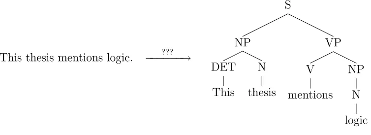
This thesis focuses on the task of sentence parsing,i.e., calculating the most plausible phrase structure tree (parse) for a given sentence (cf. Figure 1.1). Parsing is often the first step of an NLP application: Once the program knows the correct parse tree of a sentence, it can more easily extract characteristic information from it, which may be utilized for semantic analysis or other NLP tasks such as machine translation.
This thesis mentions logic. −−−−−−→???
S
NP
DET
This N
thesis
VP
V
mentions NP
N
[image:7.595.93.470.502.639.2]logic
Figure 1.1: Sentence parsing
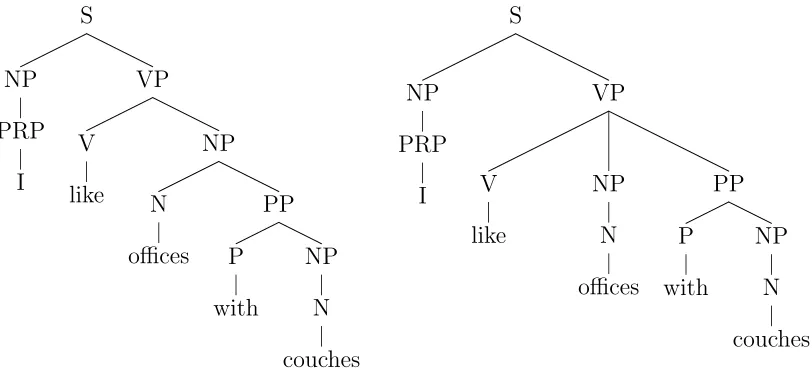
the English language, for instance, has usually many different syntactically cor-rect parses due to different possible ways of attaching prepositional phrases and relative clauses (an example is given in Figure 1.2). Humans resolve ambiguity without great difficulty; often they even fail to notice that different grammatically correct readings of the sentence exist.
S
NP
PRP
I
VP
V
like
NP
N
offices
PP
P
with
NP
N
couches
S
NP
PRP
I
VP
V
like
NP
N
offices
PP
P
with
NP
N
[image:8.595.103.509.206.392.2]couches
Figure 1.2: Two parses for the sentence “I like offices with couches.” The left one is semantically more plausible.
Statistical NLP aims at resolving ambiguities by applying statistical methods to sample data. The idea is to avoid specifying linguistic details (such as the fact that ‘table’ is a noun) directly in the program code of the NLP application, by having this application learn such details in context from a training corpus—for instance a treebank consisting of thousands of sample parse trees in the case of a parsing application. By analyzing groups of characters, words, subtrees, or other phenomena in the training data, the NLP application extracts pieces of evidence (events) and assigns probabilities to them, which allows ambiguity resolution.
In statistical parsing, the problem of grammatical ambiguity is tackled by assigning degrees of likelihood to parses. The preferred parse for a given sentence is then chosen as the one amongst all grammatically possible parses, that is most likely under the given assignment. Usually, a statistical parser utilizes an underlying probability distribution over the set of possible parse trees, according to which it chooses the most probable parse tree(s) for a given input sentence as the preferred one(s). This probability distribution is often determined by a
stochastic grammar, consisting of:
trees that can be derived from a start symbol ‘S’ by a successive application of grammar/rewrite rules, and
2. a weight assignment function associating each rule with a real number.
The probability of a parse tree is then given by the weights assigned to the rules of its possible derivations from the stochastic grammar. An example of a stochastic grammar is a Probabilistic Context-Free Grammar (PCFG) [Booth, 1969]: Its symbolic backbone is a Context-Free Grammar with rules such as ‘S→NP,VP’, ‘NP→DET N’, or ‘N→Mary’, yielding a language of phrase-structure trees. The weights associated with the rules are real numbers in the interval [0,1]. The probability of a parse tree in the language is now defined as the product of the weights of the rules that were applied to obtain its (left-most) derivation.
In the early stages of statistical parsing, grammars were manually de-signed by grammarians depending on the specific task and domain of the project. The weights of the grammar rules were then obtained automati-cally from a training corpus, consisting either of natural-language utterances [Baker, 1979, Fujisakiet al., 1989, Lari & Young, 1990, Jelinek et al., 1990] or phrase-structure trees [Pereira & Schabes, 1992]. Corpora of the latter type are also referred to as treebanks.
In more recent approaches, even the grammar rules themselves are obtained from the treebank [Scha, 1990, Charniak, 1993]. These so-called treebank gram-mars avoid the costly process of manually designing a grammar and tend to be more robust since they reflect the actual performance of a language user rather than her principal linguistic competence.
This thesis is aboutData-Oriented Parsing (DOP)1, a treebank-grammar ap-proach introduced by Remko Scha [Scha, 1990] and formalized by Rens Bod [Bod, 1991]. Its underlying assumption is that human perception of language is based on previous language experiences rather than abstract grammar rules. In the most prominent DOP variants, certain subtrees (calledfragments) are ex-tracted from the parse trees of the treebank during the training process. These fragments are assigned weights between 0 and 1. Fragments can be recombined to parse trees. This way,newparse trees—trees that did not necessarily occur in the training corpus—can be obtained. The probability assigned to a parse tree under DOP is determined by the weights of the fragments with which that parse tree can be built up.2
1
Pronounced: ‘dopp’. 2
Problem statement
Although already achieving state-of-the-art performance, the commonly used model DOP1 lacks a formal justification such as, e.g., the maximum-likelihood principlecommon in statistical NLP. Furthermore, it has the disturbing property of inconsistency [Johnson, 2002]: The probabilities that DOP assigns to parse trees do not converge to the relative frequencies of these trees in the training cor-pus when that corcor-pus grows large. As we will demonstrate, the failure to fulfill this property causes DOP to incorrectly rank different possible parses for a given sentence based on the evidence in the training corpus. A related problem is the model’s bias towards fragments of large parse trees.
Aside from estimation issues, the fact that a parse tree contains an exponential number of DOP fragments in terms of the size (i.e., number of nodes) of the tree has consequences for DOP’s computational properties.Whereas PCFG-based models have algorithms for computing the most probable parse in polynomial time w.r.t. sentence length, DOP’s case is NP-complete [Sima’an, 1999] and is dominated by the huge size of the grammar.
Contributions
We devise a new DOP model that satisfies the property of consistency. The difficulty lies in the problem that the maximum-likelihood method, according to which the joint probability of the parse trees in the training corpus should be maximized, an estimation method often leading to consistency, is not suitable for DOP: Standard maximum-likelihood estimation results in an overfitted (though consistent) estimator that only learns the parses directly occurring in the training data [Bonnema et al., 1999].
In this thesis, we follow a generalized maximum-likelihood approach leading to the first nontrivial consistent estimator for DOP. Our estimator DOP∗ ap-plies held-out training: Grammar productions are extracted from one part of the training corpus, and their probabilistic weights are assigned based on their participation in derivations of trees from a distinct, held-out, part of the corpus. While the formula for those weight assignments is derived from the optimization problem of maximizing the likelihood of the held-out corpus, a simplifying as-sumption is introduced during the solution process. This asas-sumption leads to a computationally inexpensive closed-form solution and at the same time causes DOP∗ to prefer learning simpler derivations of parses during the training process. As a side product of the estimation mechanism, the estimator learns only a number of fragments that is linear in the total number of nodes of the trees in the training corpus, thereby circumventing the inefficiency problems of original DOP without giving up on the idea of using arbitrary-size fragments.3
3 DOP∗
conver-Another property of estimators often considered to be desirable is being un-biased. We show that DOP estimators cannot—and should not be—completely unbiased. However, we will demonstrate that in contrast to DOP1, DOP∗ is not biased towards fragments of large parse trees.
Last but not least, we empirically validate our theoretical findings. Using the OVIS corpus to compare the performance of the DOP∗ parser to DOP1, we find that DOP∗ achieves better results in parsing accuracy.
1.1
Outline
The following chapter paves the ground for this thesis by acquainting the reader with basic concepts used in statistical parsing. We introduce the Data-Oriented Parsing framework, point out shortcomings of the standard model, and review previous attempts of addressing these shortcomings. Further, the paradigms of
maximum-likelihood estimationand held-out estimation are introduced.
In Chapter 3, we introduce the notions of an estimator, bias, and consistency, and then examine how bias and consistency apply to DOP. We will show that every reasonable DOP estimator must be biased, give a proof that the DOP maximum-likelihood estimator is consistent in preparation for the consistency proof for DOP∗, and informally ascertain necessary conditions a consistent DOP estimator must fulfill.
Chapter 4 presents the new estimation procedure DOP∗. The chapter also includes a consistency proof for DOP∗. Further, we show that DOP∗ can achieve an exponential reduction in the number of fragments extracted from the training corpus w.r.t. DOP1 and argue that in contrast to DOP1, DOP∗ is not biased towards fragments of large full parse trees.
Chapter 5 substantiates the theoretical findings of this thesis with empirical evidence. Concluding remarks and directions for possible future work are given in Chapter 6.
Chapter 2
Background
As indicated in the introduction, statistical-NLP algorithms extract pieces of evidence (often called: events) from a training corpus and assign weights to them based on their frequency in the corpus. A probabilistic model1 then provides a method of combining events to obtain samples (e.g., sentences or parse trees) and assigns a probability to each sample based on the weights of the events from which the sample was assembled.
Perhaps the simplest example for a probabilistic model is the unigram model
over word sequences. Here, the samples are natural language sentences and the events extracted from the training corpus are words and the end-of-sentence mark dot. The model assigns to each eventeits relative frequencyrf (e) of occurrence in the training corpus. The probability of a sentence (regarded as a sequence
hw1, . . . , wn,doti, where n∈IN andw1, . . . , wn are word-events2) is now simply
defined as the product of the weights of its events:
Punig(hw1, . . . , wn,doti) = rf (w1)· · ·rf (wn)rf (dot) .
It is easy to show thatPunig is a probability distribution over the set of possible
sentences.
A probabilistic model for statistical parsing uses parse trees (cf. Figure 1.1) as samples. In the case of Data-Oriented Parsing, events are subtrees that can be combined using a substitution operation.
This chapter starts out with some basic concepts used in statistical parsing and establishes the notation used throughout this thesis (Section 2.1). Subse-quently, we introduce the Data-Oriented Parsing framework, advert to shortcom-ings of the standard model, and review previous attempts of addressing these shortcomings (Section 2.2). In the remaining sections, two methods of assigning
1
Not to be confused withprobability models as introduced in Section 2.3. 2
weights to events commonly used in statistical NLP, maximum-likelihood esti-mation and held-out estimation, are introduced to prepare the ground for the subsequent chapters.
2.1
Terminology
In this section, we introduce notation that will be employed throughout this thesis.
Sentences and trees
In statistical NLP, the basic units considered are usually the words of a fixed natural language. A sentence is formally treated as a sequence of words.
When writing about trees in this thesis, we mean phrase structure trees, that is, trees whose non-leaf nodes are phrase-structure categories (e.g., ‘S’, ‘NP’, ‘N’) and whose leaves are either categories or words. Sometimes, the words of a phrase structure tree are also referred to asterminals and the categories asnonterminals, alluding to the terminology of Formal Language Theory. A tree with root node ‘S’ (the start nonterminal) all of whose leaves are words and in which ‘S’ does not occur in any non-root node is called a full parse tree (also: parse tree, or simplyparse). A parse tree for a given sentence s is a full parse tree whose yield (i.e., its sequence of leaves traversed from left to right) is the sentence s. Confer Figures 1.1 and 1.2 for examples of full parse trees.
Sequences
When talking about sequences, we mean finite sequences. The symbol ◦ de-notes the composition operation for sequences, |s| the length of a sequence s. When using set operators such as ∈,∩,∪, etc., on a sequence, they refer to the induced set of all the elements occurring in the sequence. For a sequence
s, we write Counts(e) for the number of occurrences of the element e in s,
and rfs(e) = Counts(e)
|s| for e’s relative frequency in s. We extend those
defini-tions to sets E of elements by defining Counts(E) := Pe∈ECounts(e) and rfs(E) :=Pe∈Erfs(e).
Finally, given a set S, the star of S is defined as
S∗ := [
i∈IN
Probability distributions over parse trees
Wherever we come across probability distributions in this thesis, their underlying sample space will be the setParses of all full parse trees. Since this set is count-able, we can characterize a probability distribution overParsesby its probability function, a function from Parses to [0,1] assigning to each elementary event{t}
(where t ∈ Parses) its probability, and will from now on sloppily talk about probability distributions P :Parses→[0,1].
Corpora and experimental methodology
Atreebank is a sequence of full parse trees, which are assumed to be independent samples from Parses according to a certain probability distribution. Note that this view—fundamental to DOP1 as well as DOP∗—completely neglects inter-sentence dependencies such as discourse phenomena.
For experiments, the treebank is split into atrainingand atesting corpus. The former is used during the training process, while the latter is a reserved portion of the treebank—not seen during training—, whose sentences (extracted from the leaves of the parse trees) are fed into the parser in order to compare its proposed parse with the parse tree the test sentence was attached to. This practice leads to objective performance figures, which make different parsers comparable to each other.
Estimation
The training procedure in statistical parsing results in a probability distribution over Parses, according to which the parser can determine the preferred parse for an input sentence. We will call this procedure an estimator. Intuitively, an estimator tries to approximate the ‘true’ probability distribution assumed to underly the training corpus. In the case of DOP, the estimator is the procedure that assigns weights to fragments and thereby probabilities to full parse trees dependent on the training corpus. An estimator is consistent if its estimated probability distribution converges to the ‘true’ distribution when the training corpus grows large. We will give a formal definition of an estimator and its properties in Chapter 3.
2.2
Data-Oriented Parsing
[Scha, 1990, Bod & Scha, 1996, Bod, 1998]. In Subsections 2.2.3 and 2.2.4, we advert to shortcomings of the standard model. Subsection 2.2.5 gives an overview and assessment of previous attempts of addressing these shortcomings.
2.2.1
The General Framework
As already mentioned in the introduction, during the training process of DOP,
fragments (also simply called subtrees) are extracted from the full parse trees of the training corpus. For each full parse tree t, the multiset of fragments of t is the multiset of all occurrences of subgraphsf of t, such that
1. f consists of more than one node,
2. f is connected,
3. each non-leaf node in f has the same daughter nodes as the corresponding node int.
For instance, the fragment multiset of the tree S A b A b is S A b A b , S A A , S A b A , S A A b ,A b , A b .
For a given training corpus tc =ht1, . . . , tNi, its fragment corpus Fragtc is the
composition of the sequences s1, . . . , sN, where si is the sequence resulting of
arranging the elements of the fragment multiset of ti according to some fixed
order. We denote the set induced byFragtc asFragSettc. Using the convention introduced in Section 2.1, we will avoid referring to that set explicitly wherever possible. A fragmentf ∈ Fragtc is called a proper fragment w.r.t. tc if it does not occur as a full parse tree intc.
In the next step of the DOP estimation procedure, each fragmentf ∈Fragtc
is assigned a weight π(f)∈ [0,1] such that the weight assignment to fragments with a common root R forms a probability distribution for each R occurring as a root inFragtc. In other words, for each suchR,π must fulfill the condition
X
f: root(f)=R
As mentioned earlier, DOP allows for the recombination of fragments to new full parse trees. This is done by tree composition. The composition of tree t1 and tree t2, resulting in the tree t1 ◦t2, is defined iff the leftmost leaf of t1 that is a nonterminal is identical to the root of t2. If defined, t1◦t2 yields a copy of
t1 whose leftmost nonterminal leaf has been replaced by the whole treet2. Note that this composition operation is technically not associative.3 When writing
t1◦t2◦t3, we mean (t1◦t2)◦t3.
A sequencehf1, . . . , fni ∈(Fragtc)nsuch thatt =f1◦· · ·◦fnis a full parse tree
is called a derivation of t. The DOP probability of a derivation d =hf1, . . . , fni
is the product of the weights of the involved fragments:
Pdop(d) :=
n
Y
i=1
π(fi)
The property that weights of fragments with the same root sum up to one ensures that Pdop is a probability distribution over the set of all derivations.4 The DOP probability of a full parse tree is now simply defined as the sum of the DOP probabilities of all its derivations. TheDOP probability of a sentencein turn is the sum of the DOP probabilities of its full parse trees. Finally, thepreferred parse(s)
according to DOP is/are the full parse tree(s) with maximal DOP probability.
2.2.2
The DOP1 Estimator
The DOP1 estimator is obtained by choosing the weight assignment π to frag-ments such that each fragment f ∈ Fragtc is assigned its relative frequency amongst all occurrences of fragments with the same root in Fragtc:
π(f) := CountFragtc(f)
CountFragtc({f0 ∈Fragtc |root(f0) = root(f)})
A toy example of a training corpus, its resulting fragment corpus, the weights assigned by DOP1, and the calculation of the DOP1 probabilities of some result-ing full parse trees is given in the followresult-ing subsection.
2.2.3
DOP1 Is Inconsistent
DOP1 suffers from some severe problems. One of them is the inconsistency of the estimation method. Consider a training corpus in which only the two parse
3
However, we have (t1◦t2)◦t3=t1◦(t2◦t3) if both sides of the equation are defined. 4
trees drawn in Figure 2.1 occur, both with equal frequencies. The treest1 and t2 have the same structure and differ merely in the categories assigned to the words “a” and “b”. Intuitively, neither of them should be preferred as a parse for the sentence “a b.”
: 2:
1 S S t Z a Z Y X a t
[image:17.595.196.395.180.229.2]b b
Figure 2.1: Two analyses for the sentence “a b”
Z S Z Z b S Z Z a S Z Z b a
S Z
b Z a Z Y X S Y X b S Y X a S Y X
a b S
b
X Y
a
1/8 1/8 1/8 1/8
1/8 1/8
1/8 1/8
1 1
1/2 1/2
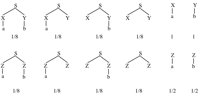
Figure 2.2: The fragments extracted from the “a b” training corpus and their DOP1-weights
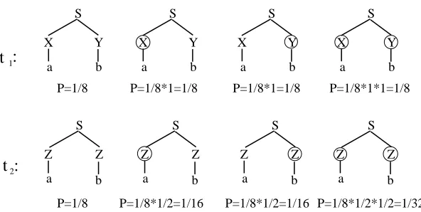
Figure 2.2 shows the fragments of the resulting fragment corpus and their weights assigned by DOP1. In order to calculate the DOP1 probabilities of t1 and t2 (as can easily be seen, they are the only parses for “a b”), we need to determine all of their derivations and their respective DOP1 probabilities. This has been done in Figure 2.3. Here and in the following, we use the convention to denote a derivation of a full parse tree by the tree itself, in which the nodes at which the compositions of fragments occurred are marked.
Now we can determine the DOP1 probabilities of t1 and t2 by summing up the probabilities of their derivations:
PDOP1(t1) = 1 8 + 1 8 + 1 8 + 1 8 =.5
PDOP1(t2) = 18 +161 +161 +321 =.28125 (2.1)
[image:17.595.130.458.288.446.2]S
Y X
a b
S
Y X
a b
S
Y X
a b
S
Y X
a b
[image:18.595.156.452.104.253.2]Z S a Z b Z S a Z b Z S a Z b Z S a Z b : 2 t P=1/8*1/2*1/2=1/32 P=1/8*1/2=1/16 P=1/8*1/2=1/16 P=1/8 : 1 t P=1/8*1*1=1/8 P=1/8 P=1/8*1=1/8 P=1/8*1=1/8
Figure 2.3: The derivations of t1 and t2 and their probabilities
Let us now assume that the trees in the training corpus were sampled accord-ing to an underlyaccord-ing probability distribution P with P(t1) = P(t2) = 0.5.5 Even when the size of the training corpus sampled according to P grows very large (and thus, the relative frequencies of t1 and t2 will be roughly 0.5), DOP1 will keep assigning them probabilities close to the ones in Equation 2.1. Intuitively, the DOP estimator should choose the weights it assigns to the fragments in such a way that the resulting probabilities assigned to the derivable full parse trees ap-proach the relative frequencies of their occurrences in the training data when its size grows large. This requirement is made precise by the notion of consistency, which will be formally introduced in Chapter 3. The inconsistency of DOP1 was first shown in [Johnson, 2002].
2.2.4
DOP1 Is Biased Towards Fragments of Large Parse
Trees
The problem of DOP1’s inconsistency is related to another one: Its bias towards fragments of large full parse trees, illustrated in [Bonnema et al., 1999]. For a tree
t= R
t1· · ·tk
,
wheret1, . . . , tkare the subtrees under the rootR, the sizesif(t) of the multiset of
its initial fragments (that is, the fragments with the same root R), is recursively given by
sif(t) =
k
Y
i=1
(sif(ti) + 1).
5
In the case of balanced binary parse trees for instance, that means that for a tree
t(h) of height h and a tree t(h+1) of height h+ 1, we have
sif(t(h+1)) = sif(t(h)) + 1
2
.
That makes clear why in DOP1, where fragments are assigned weights propor-tionally to their numbers of occurrence in the fragment corpus, the full parse trees with the greatest height, containing a great deal more fragments than parse trees of lesser height, are unjustifiably favored.
A similar calculation shows that the fragment multiset of a given full parse tree contains considerably more fragments of a certain height than fragments of any smaller height. This bias towards large fragments was addressed in two attempts of redefining the weight assignment function. The following subsection gives a brief overview.
2.2.5
Other Existing DOP Estimators
Bonnema’s Estimator
Bonnema et al. [Bonnema et al., 1999, Bonnema, 2003] propose a DOP estima-tion method that tackles the problem of DOP1’s bias towards large fragments. We will omit its theoretical motivation here and just state the formula for the estimator directly. Let N(f) denote the number of non-root nonterminal nodes of a fragmentf. Bonnema’s DOP estimator assigns to each fragmentf from the training corpus tc the weight
π(f) = 2−N(f) CountFragtc(f)
CountFragtc({f0 ∈Fragtc |root(f0) = root(f)})
.
This way, weight mass is discounted from large fragments and distributed over smaller ones.
Is Bonnema’s estimator consistent? In [Bonnema, 2003], a proof is given from which easily follows that the estimator is consistent for PCFG distribu-tions: Given a probability distribution PG over Parses resulting from a PCFG
G, the sequence of DOP probability distributions estimated from growing train-ing corpora sampled accordtrain-ing toPG converges to PG. This is nice, but not nice
enough: the simple example treebank from Section 2.2.3, for which DOP1 was shown to be inconsistent, also causes Bonnema’s estimator to fail, as can easily be calculated.
The DOP Maximum-Likelihood Estimator
The DOP maximum-likelihood estimator DOPML is the estimator defined by the
following weight assignment to fragments f extracted from the training corpus tc:
π(f) =
rftc(f) if f is a full-parse tree intc
0 otherwise
The resulting DOP probability distribution is simply the relative frequency dis-tribution of the full parse trees in the training corpus.
We will come back to this estimator in Section 2.3. As we will see in Section 3.3, DOPML is consistent.
Back-off DOP
In the method of back-off parameter estimation for the DOP model
[Sima’an & Buratto, 2003], derivations are hierarchically structured within a so-called back-off graph. The aim is to account for the probabilistic dependencies of overlapping fragments in a principled manner (in contrast to DOP1, where simply independence is assumed in the generative model of a derivation process). In order to define the back-off graph, the notion of a DOP derivation is slightly generalized to also allow the derivation of partial parses—i.e., fragments—by a successive application of substitution steps. Further, the attention is restricted to length-two derivations, i.e., pairs of fragments. A derivation d = hf1, f2i is called a back-off of a fragment f if f =f1◦f2.
In [Sima’an & Buratto, 2003], length-two derivations form the nodes of the back-off graph. For the sake of presentation, we define the notion of a back-off graph slightly differently: A back-off graph is a directed graph whose nodes are the fragments from the training corpus and whose arrows point from fragment f
to fragmentg iffg participates in a back-off of f,i.e., ifff =g◦horf =h◦g for some fragment h. Note that this graph is acyclic since a fragmentg participating in a back-off of a fragment f is always smaller in the number of nodes than f.
The back-off graph induces a hierarchy between copies of fragments—the back-off hierarchy—as follows: The first layer consists of the sources of the back-off graph, i.e., the fragments that do not participate in any back-offs of fragments. These turn out to be the full parse trees of the training corpus. The n-th layer contains all fragmentsf for which there is a path of lengthn−1 from a source in the back-off graph to f. In other words, the n-th layer consists of the fragments that participate in back-offs of fragments from layer n−1. Note that the same fragment can occur in different layers! Since the back-off graph is acyclic and finite, the induced back-off hierarchy has always a finite number of layers.
The estimation procedure for Back-off DOP now operates iteratively in n
procedure stepwisely transfers weight mass from one layer to the next. Intuitively, this amounts to the transfer of probability mass from preferred derivations to back-off derivations of trees in the training corpus.
The particular redistribution formula is an adaption of the Katz back-off method known from n-gram smoothing. However, as opposed to Katz back-off, where different estimators are interpolated during the testing process, Back-off DOP interpolates different weight assignments to fragments during the training
process.
The original Katz smoothing formula assigns new probabilities to n-gram events based on up to n given probability distributions (usually the relative fre-quency distributions) over the set of alln-grams, the set of all (n−1)-grams, and so forth. In Back-off DOP, these n given distributions should correspond to n
given distributions over fragments—one for each of thenlayers in the back-off hi-erarchy. This confronts Back-off DOP with an inherently difficult problem: What
given distributions over fragments should be used? What meaning does a prob-ability distribution over fragments have for DOP in the first place? DOP assigns only probabilities to full parse trees, and this only indirectly: They result from weight assignments to fragments. Since the weight assignments to fragments of the same root form a probability distribution, [Sima’an & Buratto, 2003] choose to apply the back-off formula separately for each nonterminal N to fragments of rootN. Asgiven distributions, they use the weight assignments given by DOP1 and Bonnema-DOP, leading to two different variants of Back-off DOP.
We believe that
1. the back-off formula specified in [Sima’an & Buratto, 2003] does meet the intuition of assigning higher DOP probabilities to derivations from ‘pre-ferred’ fragments in top (i.e., low-numbered) layers of the back-off hierarchy and lower ones to back-off derivations from fragments in higher-numbered layers6 and
2. applying back-off smoothing to weight assignments rather than DOP prob-abilities does not take into account an event’s probability, as required in the Katz back-off formula, appropriately.
The first point is unproblematic. A slight adaption of the formula should suffice. As to the second point, how can the notion of a DOP probability, so far only defined for full parse trees, be generalized to fragments in a sensible way? In [Nguyen, 2004], the notions of aDOP derivation and its probability are general-ized to fragments. For fragments that are full parse trees, her notion of a DOP probability coincides with the original notion.
6
Unfortunately, proceeding in this way (using DOP probabilities instead of weights in the back-off formula) would lead to a system of nonlinear equations, one for each fragment occurrence in the back-off hierarchy. Sensible simplifying assumptions would be necessary.
An alternative solution could be to train n different estimators for each of the n layers in the back-off hierarchy and interpolate these estimators during the testing process, as done in the original Katz back-off estimation process. However, as Sima’an remarks (personal communication), such an estimation method would lose out considerably on DOP’s original spirit of involving all kinds of fragments in the derivation process since fragments of different layers are now strictly separated into different estimation modules and could not recombine with each other.
According to Sima’an (personal communication), it should not be too difficult to devise the back-off formula in such a way that the resulting estimator becomes consistent. In essence, the fragments of the first layer in the back-off hierarchy would have to become increasingly dominant (in terms of assigned weight mass) as the corpus gets larger and more homogenous. Even the version of Back-off DOP presented in [Sima’an & Buratto, 2003] achieves already very promising empirical results. However, the inefficiency problem of DOP1 is inherited by Back-off DOP: Since all fragments are extracted from the training corpus, parsing time does not improve over DOP1.
2.3
Probability Models and The Principle of
Maximum-Likelihood Estimation
If we look at the training process of a parsing system from the viewpoint of estima-tion theory, we can regard that process as the choice of a probability distribuestima-tion over Parses out of a certain set M (called: probability model) of acceptable probability distributions. Often, for the choice of the appropriate probability distribution, the Maximum-Likelihood Criterion is used, according to which the probability distribution that maximizes the joint probability of the full parse trees in the training corpus, the so-called Maximum-Likelihood Estimate (MLE), is chosen. If Mis unrestricted, that is, if it contains all possible probability dis-tributions over Parses, then the MLE always exists, is furthermore unique, and is identical to the relative frequency estimate (RFE)7
Prf :Parses →[0,1], where Prf(t) :=rfTC(t).
Remember here that rfTC(t) = Count|TCTC(| t) denotes t’s relative frequency in the training corpus TC.
7
Given a training corpus tc, the DOP probability model induced by tc, de-noted Mdop(tc), is the set of all DOP-probability distributions (over Parses)
resulting from weight assignments to the set of fragments in the fragment corpus
Fragtc. This model plays a role not only for the problem of finding the most suitable weight assignment to the fragments from tc, but also for considering formal properties of DOP, such as bias and consistency, which will be the aim of Chapter 3.
For now, let us come back to the problem of maximum-likelihood estimation: The DOP maximum-likelihood estimator DOPML is usually referred to as the
DOP procedure that assigns weights to the fragments extracted from the training corpus in such a way that the resulting joint DOP-probability of the training corpus is maximized [Bonnemaet al., 1999, Sima’an & Buratto, 2003]. DOPML
thus yields the maximum-likelihood estimate w.r.t. Mdop(tc). Although the
probability model is now restricted, the RFE belongs to it, and hence the MLE is still identical to the RFE. Why the RFE is a member of the probability model can easily be seen by considering the weight assignment allocating to each full parse tree its relative frequency in the training corpus and zero to all proper fragments,
i.e., fragments that are not full parse trees. All derivations remaining possible under this weight assignment are the unique length-1 derivations of the corpus trees themselves, having as their DOP probability the weight of the respective full parse, which is equal to its relative frequency.
What we also learn from this is that relative frequency estimation for DOP (and thus the DOP maximum-likelihood estimator) is of no practical use since it only assigns nonzero weights to the fragments that occur as full parse trees in the training data. This is not what we want. Natural language data is sparse, that is, many full parse trees will occur only a few times or not at all in the training data. Therefore, the RFE is unsatisfactory for statistical parsing. Not only does it assign probability 0 to all parses that do not occur in the training data. It can also only give rough estimates for rarely occurring full parse trees. There are different ways out of this common problem ofoverfitting in statistical NLP: One can either restrain the probability modelMof acceptable probability distributions from which the MLE is chosen, or modify the model (e.g. by prun-ing it [Sima’an, 1999]), or adjust the relative frequency estimate by discounting
probability mass from frequently occurring events (in our case: full parse trees) and distributing that mass over the unknown and rarely occurring events.8 The technique ofheld-out estimation, which we will encounter in the following section, belongs to the class of discounting methods. Restraining the model (in the case of DOP) can for instance be achieved by only allowing fragments up to a certain depth to have nonzero weights [Bod, 2000, Bod, 2001] or by imposing conditions
8
on the weight assignment functions, as done in Back-off DOP (cf. Subsection 2.2.5).
Where will our estimation method DOP∗ fit in? Basically, DOP∗ restrains the model by only extracting fragments from a part of the training corpus. At the same time, however, some probability mass will be reserved and distributed over fragments from the rest of the corpus.
2.4
Held-Out Estimation
Held-out estimation is a method used in n-gram based language modelling. For comprehension of the rest of this thesis, the hurried reader only needs to know its core idea of reserving a part of the training corpus (the held-out part) for some preliminary testing on how representative the training data is and can now lightheartedly jump to the next chapter.
A simple example application forn-gram modelling (or equivalently: (n−1)th order Markov modelling) is the task of predicting the next word w in a text in a natural language by considering the n−1 wordsw1, . . . , wn−1 that preceded w in the text. For this purpose, a probability distribution over n-tuples of words (called: n-grams) is estimated. This can be done by maximum-likelihood es-timation, i.e., by assigning each n-gram its relative frequency of occurrence in the training corpus tc. We have already encountered a related version of this estimation method for the casen= 1 (unigrams) at the beginning of this chapter. The probability for a wordw to occur after a word sequence w1. . . wn−1 can now be calculated as
P(w|w1. . . wn−1) =
P(w1. . . wn−1w)
P(w1. . . wn−1)
= Prftc(w1. . . wn−1w)
w0rftc(w1. . . wn−1w0)
As we have seen in the previous section, relative frequency estimation is inca-pable of dealing with unknown events (here, n-grams). Therefore, in held-out estimation, some probability mass is discounted in a certain way from all known
n-grams (i.e.,n-grams that occurred during training) and evenly distributed over the unknown ones. Here, unknown n-grams are meant to be n-grams from the setNGrams which are not known, whereNGrams is defined dependent on the training data as the set of n-tuples of the set of words from the training cor-pus. The set NGrams is therefore always finite, whence it is possible to evenly distribute the discounted probability mass over the unknown n-grams.
n-grams as explained above. Then the held-out corpus is considered in order to estimate how often n-grams that occurred r times actually happen to occur during testing. This yields an estimate of the expected relative frequency of an
n-gram during testing and thus of its actual probability.
Let r =Countatc(t) be the number of occurrences of a certain n-gram t in
atc. Then we define
Tr :=
X
t0:Countatc(t0)=r
Counthc(t0)
to be the total number of times that n-grams occurring r times in the actual training data occur in the held-out data. Dividing Tr by the number Nr of
distinctn-grams appearing exactly r times in the actual training data yields the average frequency that such n-grams have in the held-out data. This value is called the held-out discount erho of r:
e
rho :=
Tr
Nr
, where Nr :=|{t0 ∈NGrams|Countatc(t0) =r}|
Note that for unknown n-grams t (i.e., r = 0), N0 is the number of distinct n -grams not occurring inatc,i.e., the number of distinct unknownn-grams. Note also that although dubbed ‘discount’,reho can actually be greater than reven for
r≥1.
The held-out discount still depends on the size of the held-out data. Dividing by that size yields a held-out estimate of the relative frequency with which ann -gram occurs in actual testing data, and thus an improved estimate of ann-gram’s probability as compared to relative frequency estimation:
Pho(t) := reho
|hc|, wherer =Countatc(t) (2.2)
It is easy to check that Pho is a probability distribution over NGrams.
Unfortunately, held-out estimation is not straight-forwardly applicable to DOP, the reason being that it is ultimately based on relative frequency esti-mation. Relative frequency estimation for DOP is of no use since it only assigns probability mass to full parse trees directly occurring in the training data. Held-out estimation applied to DOP would just distribute the reserved probability mass evenly over all ‘unknown’ parse trees (where the definition of ‘unknown’ would here have to be adjusted in order to make the set of all unknown parses finite), treating them all completely equally. The actual strength of DOP, lying in the way it combines evidence for full parse trees found in the training data in order to predict the existence of similar full parse trees which have not occurred during training, would be completely ignored by held-out estimation.
Chapter 3
Considerations about Bias and
Consistency
In this chapter, we will introduce the notion of an estimator and the properties of bias and consistency. Subsequently, we examine how bias and consistency apply to DOP. We will show that every reasonable DOP estimator must be biased (Sec-tion 3.2), give a proof that the DOP maximum-likelihood estimator is consistent in preparation for the consistency proof for DOP∗ (Section 3.3), and informally ascertain necessary conditions a consistent DOP estimator must fulfill (Section 3.4).
3.1
Basic Notions
In the following, we will establish the notion of an estimator and some of its properties. An introductory treatment of estimation theory is for instance given in [DeGroot & Schervish, 2002], Chapter 6; [Krenn & Samuelsson, 1997], Section 1.7; or [Siegrist, 2004]. However, in statistical parsing, we are interested in the estimation of whole probability distributions, not merely real-valued parameters or parameter vectors in Rn, as in standard estimation theory. Therefore, the standard definitions have to be slightly adapted.
3.1.1
Estimation
of DOP, the estimator is the procedure that assigns weights to fragments and thereby probabilities to full parse trees dependent on the training corpus.
Usually, assumptions are made on the kind of probability distributions that can underly the training data. This translates to fixing a model in the jargon of estimation theory: The training corpus is assumed to have been sampled from a probability distribution in a fixed model M(cf. Section 2.3).
Assume thus we are given a model M of probability distributions over the sample space Parses and a probability distribution P ∈ M, according to which independent samples, observations, are drawn. An estimator tries to predict
P from the observation sequence—a sequence of random samples from Parses
according to the probability distribution P, in the case of DOP the training corpus. The actual definition of an estimator is independent of M:
Let M0 denote the unrestricted probability model over Parses (cf. Section 2.3). An estimator ϕ : Parses∗ → M0 is a function that assigns a probability distribution (the estimate) to a finite sequence of samples from Parses.1
The modelM will become important when we consider properties ofϕ, such as bias and consistency. The model-independent definition of an estimator also enables us to consider properties of one estimator w.r.t. different underlying models, which we will actually do later.
In the following, we will sometimes denote the estimateϕ(s) for an observation sequences=ht1, . . . , tni ∈Parsesn asϕs to stress the fact that it is a probability
distribution.
3.1.2
Bias, Loss Function, and Consistency
In the following definitions, we adhere to [Johnson, 2002], where the inconsistency of DOP1 was first proved, using slightly simplified notation.
Let X = hX1, . . . , Xni be a sequence of n independent random variables
distributed according to a probability distribution P in the model M. Then the estimate ϕ(X) is a random variable as well, ranging over the probability distributions in M0. It is easy to see that the expected value of the probability distribution assigned by ϕ,
EP [ϕ(X)] =
X
ht1,...,tni∈Parsesn
P(t1)· · ·P(tn)ϕ(t1, . . . , tn),
is also a probability distribution over Parses.
1
Recall that for a setS,S∗:=S
i∈INS
i
Bias
Based on the expected value of ϕ(X), we define the estimator ϕ to be biased
for some probability distribution P over Parses if there is an n ∈ IN such that for the sequence X =hX1, . . . , Xni of independent random variables distributed
according toP,
EP [ϕ(X)]6=P
holds. We call ϕ biased w.r.t. Mif it is biased for some P ∈ M.
Loss
A loss function L is a mapping from M2
0 to the nonnegative reals. The value
L(P, ϕ(t1, . . . , tn)) expresses the loss incurred by the error made in the estimate
ϕtc of P from the sample sequence tc=ht1, . . . , tni.
The expected loss for an estimation of P from a sequence of observations of lengthn,
EP[L(P, ϕ(X1, . . . , Xn))]
is called therisk of ϕ at P for sample size n.
Consistency
The estimatorϕ is called consistent w.r.t. Mif for each probability distribution
P ∈ M, the risk ofϕ atP approaches zero when the sample size goes to infinity,
i.e., if we have
lim
n→∞EP [L(P, ϕ(X1, . . . , Xn))] = 0
for all P ∈ M.
The question remaining is: What loss function should we choose in order to obtain a sensible definition of consistency? We follow [Johnson, 2002] by defining
L(P, ϕ(t1, . . . , tn)) :=
X
t∈Parses
P(t) [P(t)−ϕ(t1, . . . , tn)(t)]2 .
Note that the function value is always in [0,1] since
0≤[P(t)−ϕ(t1, . . . , tn)(t)]2 ≤1.
Writing out the formula for the expected loss, ϕ is thus consistent w.r.t. Miff
lim
n→∞
X
tc∈Parsesn
P(tc) X
t∈Parses
P(t) [P(t)−ϕtc(t)]
2
= 0 for all P ∈ M,
whereP(tc) =P(t1)· · ·P(tn) is the probability of the sequencetc=ht1, . . . , tni
Strong consistency
In the literature, consistency is often defined more directly in terms of an ad-missible error ε. An estimator is then considered consistent if for each ε > 0, its estimate deviates from the true parameter by more than ε with a probability approaching zero when the sample size approaches infinity. A possible adaption of this view of consistency to our framework of statistical parsing is given by the following definition:
LetMandϕbe given as specified above. Thenϕ is calledstrongly consistent w.r.t. M if for eachP ∈ M and each real number ε >0, we have
lim
n→∞t∈Parsessup
X
tc∈Parsesn:
|ϕtc(t)−P(t)|≥ε
P(tc) = 0.
3.1.3
Strong Consistency Implies Consistency
As our denotation suggests, strong consistency implies consistency:
Theorem 3.1.1 Let M be a probability model over Parses and
ϕ :Parses∗ → M0 an estimator.
If ϕ is strongly consistent w.r.t. Mthen ϕ is also consistent w.r.t. M.
Proof: Assume that ϕ is strongly consistent w.r.t. M. Further, let P be a probability distribution in M. We have to show:
lim
n→∞
X
tc∈Parsesn
P(tc) X
t∈Parses
P(t) [P(t)−ϕtc(t)]
2 = 0
Assume thus, we are given ε0 >0. Now defineε :=pε0/2 andq :=ε0/2. Since ϕ
is strongly consistent w.r.t. M, there is an N ∈IN such that for all n ∈IN with
n ≥N, we have
sup
t∈Parses
X
tc∈Parsesn:
|ϕtc(t)−P(t)|≥ε
P(tc)≤q
and hence
X
tc∈Parsesn: |ϕtc(t)−P(t)|≥ε
and hence
X
tc∈Parsesn
P(tc) X
t∈Parses
P(t) [P(t)−ϕtc(t)]
2
= X
t∈Parses
P(t) X
tc∈Parsesn
P(tc) [P(t)−ϕtc(t)]
2
≤ sup
t∈Parses
X
tc∈Parsesn
P(tc) [P(t)−ϕtc(t)]
2
≤ sup
t∈Parses
"
X
tc∈Parsesn: |P(t)−ϕtc(t)|<ε
P(tc) [P(t)−ϕtc(t)]
2
| {z }
<ε2
| {z }
<ε2
+ X
tc∈Parsesn:
|P(t)−ϕtc(t)|≥ε
P(tc) [P(t)−ϕtc(t)]
2
| {z }
≤1
| {z }
≤qby (3.1)
#
≤ ε2+q=ε0 .
qed
We conjecture that the other direction also holds,i.e., that the properties of consistency and strong consistency are actually equivalent. Be that as it may, in the consistency proofs given in this thesis, we will show strong consistency, and thereby also consistency, of the respective estimators.
3.2
A Short Word on Bias
probabilities to full parse trees not occurring in the training data. We start with a theorem that gives a necessary condition for a (general) estimator to be biased for a particular probability distribution.
Theorem 3.2.1 Let ϕ:Parses∗ → M0 an estimator for which there is a
train-ing corpus tc=ht1, . . . , tni ∈Parsesn and a full parse treet0 outside the corpus
(i.e., t0 6=ti (i= 1, . . . , n)) such that
ϕtc(t0)>0.
Then ϕ is biased for each probability distribution P over Parses that as-signs a positive probability to tc but a zero-probability to t0, i.e., for which
P(t1)· · ·P(tn)>0 and P(t0) = 0.
Proof: Let ϕ and tc = ht1, . . . , tni be given as specified above and assume
ϕ is unbiased for some probability distribution P with P(t1)· · ·P(tn) > 0 and
P(t0) = 0. This means that
EP(ϕ(X1, . . . , Xn)) =
X
hω1,...,ωni ∈Parsesn
P(ω1)· · ·P(ωn)ϕ(ω1, . . . , ωn) = P. (3.2)
Thus, we have X
ω∈Parses: P(ω)6=0
X
hω1,...,ωni ∈Parsesn
P(ω1)· · ·P(ωn)ϕ(ω1, . . . , ωn)(ω) =
X
ω∈Parses: P(ω)6=0
P(ω). (3.3)
Since Pω∈Parses:P(ω)6=0P(ω) = 1, we obtain from (3.3): X
ω∈Parses: P(ω)6=0
X
hω1,...,ωni ∈Parsesn
P(ω1)· · ·P(ωn)[ϕ(ω1, . . . , ωn)](ω) = 1, (3.4)
i.e., X
hω1,...,ωni ∈Parsesn
P(ω1)· · ·P(ωn)
X
ω∈Parses:
P(ω)6=0
[ϕ(ω1, . . . , ωn)](ω) = 1. (3.5)
Since X
hω1,...,ωni ∈Parsesn
P(ω1)· · ·P(ωn) = 1
and X
ω∈Parses:
P(ω)6=0
[ϕ(ω1, . . . , ωn)](ω)≤1,
Equation (3.5) can only be valid if P{ω∈Parses: P(ω)=06 }[ϕ(ω1, . . . , ωn)](ω) = 1
for all ω1, . . . , ωn ∈ Parses such that P(ω1)· · ·P(ωn) > 0. But this means
[ϕ(ω1, . . . , ωn)](ω) = 0 for all ω, ω1, . . . , ωn ∈ Parses with P(ω) = 0 and
Now we apply the theorem to DOP. The following corollary states that, given a training corpus tc and a DOP estimator that is unbiased w.r.t. tc’s induced DOP probability model2 M
dop(tc), the estimator is bound to completely overfit
the training corpus by assigning zero-probabilities to all full parse trees outside the corpus.
Corollary 3.2.2 Let there be a training corpus tc ∈Parsesn and a DOP esti-mator ϕ : Parses∗ → M0 that is unbiased w.r.t. Mdop(tc). Then ϕtc(t) = 0 for all t∈Parses with t /∈tc.
Proof: Assume indirectly thatϕtc(t0)>0 for some full parse tree t0 that is not
intc. As shown in Section 2.3, the relative frequency estimate
Prftc :Parses →[0,1], where (3.6)
Prftc(t) :=rftc(t) (3.7)
is an instance ofMdop(tc). Since rftc(t) >0 for all t ∈ tc and rftc(t0) = 0,
it follows from Theorem 3.2.1 that ϕ is biased for Prftc. Thus ϕ is biased w.r.t.
Mdop(tc). qed
It might be of interest to apply Theorem 3.2.1 to other estimators in statistical NLP. As pointed out in [Prescher et al., 2004], the theorem isnotof relevance to probabilistic context free grammars (PCFGs) since the PCFG modelMpcfg(tc)
induced by a training corpus tcdoes not contain a probability distribution that assigns positive probabilities to the trees in tc and zero to an outside tree.
3.3
The DOP Maximum-Likelihood Estimator
Is Consistent
Although it is generally accepted that the DOP maximum-likelihood estimator DOPML, introduced in Subsection 2.3, is consistent, no such proof exists in the
literature so far. Remember that DOPML assigns each full parse tree its relative
frequency in the training corpus and is thus identical to the relative frequency estimator. Relative frequency estimation for DOP differs from standard textbook RFE in that a DOP estimator does not estimate one single real-valued param-eter or a paramparam-eter vector in Rn of a probability distribution, but rather the probability distributionitself. Therefore, the results for standard RFE cannot be utilized.
In the following, we will give a proof that DOPML is consistent. We will
actually show that the estimator isstronglyconsistent—not only w.r.t. the prob-ability model Mdop(tc) induced by a given training corpus tc (cf. Section 2.3)
2
but even w.r.t. the unrestricted model M0 of all probability distributions over
Parses. The core part of the proof can be employed in the consistency proof of DOP∗ given in the next chapter and is therefore stated separately as a lemma.
Lemma 3.3.1 Let P be a probability distribution over Parses. Then for each full parse tree t ∈ Parses, natural number n ∈ IN and real value ε >0, it holds
that X
tc∈Parsesn:
|rftc(t)−P(t)|≥ε
P(tc)≤ 1
4nε2 .
Proof: LetP,t,nand εbe defined as above. Chebyshev’s inequality states that for any real-valued random variable X on Parsesn with expected value µ and variance σ2 and any ε0 >0, we have
P(|X−µ| ≥ε0)≤ σ
2
ε02 ,
i.e.,
X
tc∈Parsesn: |X(tc)−µ|≥ε0
P(tc)≤ σ
2
ε02 .
The relative frequency rftc(t) of t in tc is a random variable on Parsesn with the expected value µ = p and the variance σ2 = p(1−p)/n, where p = P(t). Thus, applying Chebyshev’s inequality yields
X
tc∈Parsesn:
|rftc(t)−P(t)|≥ε
P(tc)≤
≤1/4
z }| {
P(t)[1−P(t)]
nε2 ≤ 1 4nε2 .
qed
Now we are ready for the consistency theorem:
Theorem 3.3.2 DOPML is strongly consistent w.r.t. the model M0 of all
prob-ability distributions over Parses.
Proof: First note that the estimate DOPML(tc) is a probability distribution
assigning each full parse tree t ∈ Parses its relative frequency rftc(t). Now let P be a probability distribution over Parses and ε and q two positive real numbers. We will give anN ∈IN such that for each n∈IN with n≥N, we have
sup
t∈Parses
X
tc∈Parsesn:
|rftc(t)−P(t)|≥ε
From that follows the claim.
DefineN to be the smallest natural number such thatN ≥ 4ε12q. Then Lemma 3.3.1 yields for all n≥N and t ∈Parses
X
tc∈Parsesn:
|rftc(t)−P(t)|≥ε
P(tc)≤1/(4nε2) | {z }
≥4ε2N
≤q .
Equation (3.8) follows immediately. qed
3.4
Contemplation
Let us pause for a moment and ponder which kind of DOP estimators can ac-tually achieve consistency. In the case of DOP, consistency means that when the size of the training corpus approaches infinity, the estimator’s assignments of probabilities to full parse trees must converge to their relative frequencies in the training corpus. That is because the loss function approaches zero only if the DOP probability distribution assigned by the estimator approaches the ‘true’ distribution underlying the training corpus. But that distribution on its part is approached by the relative frequency distribution of the full parse trees in the training corpus when its size goes to infinity.
When the probability distribution assigned by the DOP estimator approaches the relative frequency distribution of the parse trees in the training corpus, this means that the probability assignments for all parse trees not found in the training corpus have to approach zero. This, however, should not happen too early (i.e., when the sample size is not large enough), otherwise the estimator would overfit
Chapter 4
The New Estimator
DOP
∗
In the last section of the previous chapter, we have seen that the DOP probability distribution assigned by a consistent DOP estimator must approach the relative frequency distribution of the parse trees in the training corpus when the corpus size goes to infinity, and that the probability assignments for all parse trees not found in the training corpus therefore have to approach zero. We will now devise a DOP estimator DOP∗ which will have the property that as the training sample size approaches infinity, the probabilities assigned to derivations of length greater than one approach zero, while the weights (and thereby the probabilities) assigned to the full parse trees from the training corpus converge to their relative frequencies.
In Section 4.1, the DOP∗ estimation procedure is explained. A consistency proof for DOP∗ is given in Section 4.2. Further, we show that DOP∗ can achieve an exponential reduction in the number of fragments extracted from the training corpus w.r.t. DOP1 (Section 4.3) and argue that in contrast to DOP1, DOP∗ is not biased towards fragments of large full parse trees (Section 4.4).
4.1
The
DOP
∗Estimation Procedure
As we have seen in Section 2.3, the standard method of maximum-likelihood estimation, according to which the joint probability of the full parse trees in the training corpus should be maximized, is not suitable for DOP. Given a training corpus tc, the MLE over Mdop(tc) assigns nonzero probability only to the full
parse trees occurring directly in the training corpus, leading to an overfitted
parser that can only reproduce the parses that occurred during training.
method of division is certainly of relevance, and we will come back to it in Chap-ter 5.) While fragments are extracted from the trees in ec, their weights are assigned such that the likelihood of the held-out corpushcis maximized. It can happen that a full parse tree inhcis not derivable from the fragments ofec(we will say that it is not ec-derivable). Therefore, we will actually maximize the joint probability of theec-derivable trees in hc.
Crucially, to avoid Expectation-Maximization algorithms such as Inside-Outside [Baker, 1979] for approaching the MLE over hc1, we will make the fol-lowing simplifying assumption: maximizing the joint probability of the full parse trees in hc is equivalent to maximizing the joint probability of their shortest derivations. This assumption turns out handy for several reasons:
• It leads to a closed-form solution for the MLE, which is further computa-tionally very inexpensive.
• The resulting estimator will only assign nonzero weights to a number of fragments that is linear in the number of depth-1 fragments (i.e., PCFG rules) contained in hc, thereby resulting in an exponential reduction of the number of fragments in the parser. Therefore, the resulting parser is considerably faster than a DOP1 parser.
• The estimator, although not truly maximum likelihood, is consistent.
The assumption also serves a principle of simplicity: A shorter derivation seems a more concise description of a full parse tree than a longer one; thus the short-est derivation can be regarded as the preferred way of building up a full parse tree from fragments, and the longer derivations as provisional solutions (back-offs) that would have to be used if no shorter ones were available. Further-more, there are empirical reasons to make the shortest derivation assumption: In [De Pauw, 1999, Bod, 2000, De Pauw, 2000] it is shown that DOP models that select the preferred parse of a test sentence using the shortest derivation criterion perform very well.
To ensure maximum coverage (i.e., to have the estimator assign nonzero prob-abilities to as many parse trees as possible), the estimation procedure outlined above reserves a certain proportion of the weight mass for smoothing: In a second estimation step, also fragments that did not participate in any shortest derivation
1
of hc-trees will be given some weight. For that purpose, animaginary fragment
R
♥
,
consisting only of the root R and its child terminal ‘♥’, and denoted by ♥R, is
introduced for each root R. The weight assigned to ♥R stands for the weight
mass to reserve and is chosen dependent on the relative frequency punkn of parse tree occurrences in hc that are not ec-derivable. The lower the value of punkn, the less weight mass is reserved. The smoothing algorithm then distributes for each nonterminal R the weight of the imaginary fragment ♥R over all root-R
fragments.
The DOP∗ estimation procedure thus consists of the following parts:
1. The core DOP∗ estimator, assigning weights β(f) to fragments f from the extraction corpus. Thereby, for each nonterminal R, a certain amount
β(♥R) of weight mass is reserved for the smoothing step.
2. The smoothing component, distributing the reserved weight mass β(♥R)
over all fragments from the training corpus and assigning each fragment f
the smoothing weight βsmooth(f).
3. The final weight assignmentπ to fragments f, given by
π(f) :=β(f) +βsmooth(f).
In the following subsection, we will derive the formula for the preliminary weight assignment β as a solution to the maximum-likelihood problem indicated above. How the reserved weight masses β(♥R) are determined and distributed
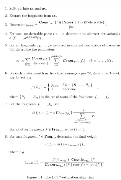
is explained in Subsection 4.1.2. Figure 4.1 gives a summary of the estimation algorithm.
4.1.1
Estimation of the
β
-weights
In order to assign the β-weights to the fragments in Fragec, derivations of full parse trees in hc using the fragments in Fragec are considered. As in held-out estimation (cf. Section 2.4), the sum of the relative frequencies of the trees in hc that are not ec-derivable is taken as the estimate punkn of the probability that a tree will be unknown during testing. Depending on punkn in a certain way de-scribed in the next section, weight mass β(♥R) for each nonterminalR occurring
as root inFragecis assigned to the imaginary fragment ♥Rand thus reserved for
1. Split tc into ecand hc.
2. Extract the fragments from ec.
3. Determine punkn =
Counthc({t∈Parses | t is ec-derivable})
|hc| .
4. For each ec-derivable parse t ∈ hc, determine its shortest derivation(s)
d1(t), . . . , d#shder(t)(t).
5. For all fragments f1, . . . , fN involved in shortest derivations of parses in
hc, determine the parameters
rk :=
X
t∈hc
Counthc(t)
#shder(t)
#shder(t) X
i=1
Countdi(t)(fk) (k = 1, . . . , N).
6. For each nonterminalRin the whole training corpustc, determineβ(♥R),
e.g. by setting
β(♥R) :=
punkn if R∈ {R1, . . . , RM}
1 otherwise ,
where{R1, . . . , RM}is the set of roots of the fragments f1, . . . , fN.
7. For the fragments f1, . . . , fN, set
β(fj) := 1−β ♥root(fj)
rj
X
k∈{1,...,N}: root(fk)=root(fj)
rk
.
For all other fragmentsf ∈Fragtc, set β(f) := 0.
8. For each fragment f ∈Fragtc, determine the final weight
π(f) :=β(f) +βsmooth(f),
wheree.g.
βsmooth(f) :=
β ♥root(f)
CountFragtc(f)
CountFragtc({f
[image:39.595.87.497.101.713.2]0 |root(f0) = root(f)}) .
to imaginary trees, that is, full parse trees that contain the terminal ‘♥’ in their yields.
How do we assign the β-weights to the fragments in Fragec based on the sample sequencehc? In the following, we will set up a maximization problem for the weight assignment functionβ, in which we regard the reserved weight masses
β(♥R) as constant (although not yet known). We derive β as the solution to
the problem of maximizing the probability of hc0 w.r.t. the model M
dop(ec),
where hc0 is the corpus obtained from hc by removing the trees that are not ec-derivable:
arg max
β∈W
Y
t∈hc: tisec-derivable
[Pdopβ(t)]
Counthc(t) , (4.1)
wherePdopβ denotes the DOP probability distribution overParsesresulting from the weight assignmentβ, andW is the set of allβ :FragSetec →[0,1] that fulfill the side conditions that for each nonterminal R in ec:
X
f∈Fragec: root(f)=R
β(f) +β(♥R) = 1 . (4.2)
Note that since the probability of a full parse tree is the sum of the DOP-probabilities of its derivations, the term to be maximized in problem (4.1) is a product of sums of products of weights. We now make the simplifying assump-tion indicated above that problem (4.1) remains equivalent when each DOP-probability Pdopβ(t) is replaced by the probability of the shortest derivation of t. (Note that it will turn out that the consistency of DOP∗ does not rely on this assumption!) If there are more than one shortest derivation for a parse (say n), we will assume that each of them derived 1/n of the occurrences of that parse, a fraction which needs not necessarily be a whole number. This leads us to the maximization problem
arg max
β∈W
Y
t∈hc: tisec-derivable
#shder(t) Y
i=1
[Pshi β(t)]Count#shder(hc(tt)) , (4.3)
where #shder(t) is the number of shortest derivations for tree t and
Pshi β(t) =β(f1(di(t)))· · ·β(flgth(di(t))(di(t)))
is the probability of the i-th shortest derivation di(t) for t, consisting of the
fragmentsf1(di(t)), . . . , f
lgth(di(t))(di(t))∈Fragec. The side conditions remain the same. Now the term to be maximized is only a product of weights. Rearranging the formula and multiplying together powers of weights of the same fragments ([β(f)]e1· · ·[β(f)]em = [β(f)]e1+···+em), we arrive at the term
arg max
β∈W
[β(f1)]r1· · ·[β(f