The long term dynamical stability of the known Neptune Trojans

The Long Term Dynamical

Stability of the Known

Neptune Trojans

A thesis submitted by

Jack Lang Soutter

For the award of

Master of Science (Research)

Abstract

The Neptune Trojans are a population of small bodies that librate around the L4 and L5 Lagrange points of Neptune’s orbit. Shortly after the discovery of the first such object, 2001 QR322, simulations suggested that the body moved on a

dynamically stable orbit. Following this, further discovered objects were generally assumed to also be stable.

In recent years, the situation has proved to be more complicated than previously thought. Two of Neptune’s Trojans have been found to exhibit orbital instability on billion year timescales, with another being revealed as a temporarily captured interloper.

Here, the results of detailed dynamical simulations of the orbital evolution of the eleven known Neptunian Trojans are presented, examining the influence of their initial orbital semi-major axes and eccentricities on their stability.

The results reveal the importance of considering the orbital stability of newly discovered objects on a case-by-case basis, with some members showing highly unstable behaviour, whilst others seem likely to be primordial in nature.

The earlier finding that 2001 QR322 and 2008 LC18 are primordial in nature but

unstable on billion year timescales are confirmed. In both cases, their stability is a strong function of their semi-major axis, with the two lying on the boundary between stable and unstable regions. In addition we reveal the stability of eight other Neptune Trojans. Six of the known Trojans move on highly stable orbits. In contrast, two objects, 2004 KV18 and 2010 EN65, are

confirmed to be temporarily captured members of the Neptune's Trojan population. While one, 2012 GX17, is found to be a misidentified

Certification of Thesis

This thesis is entirely the work of Jack L Soutter __________________except where otherwise acknowledged. The work is original and has not previously been submitted for any other award, except where acknowledged.

Student and supervisors signatures of endorsement are held at USQ.

Stephen Marsden Principal Supervisor

Jonti Horner Associate Supervisor

Acknowledgements

First of all I would like to thank my supervisors Jonti Horner, Stephen Marsden and Brad Carter for all their help and assistance through my Masters, it has been a long and rocky ride. I would especially like to thank Jonti for introducing me to the topic of Neptune Trojans, and guiding me through background and software.

I would also like to thank Matthew Mengel for his assistance with USQ's supercomputers, our entire research group owes this man an endless round of drinks.

Table of Contents

Abstract...i

Acknowledgements...iii

1. Introduction...1

1.1 The Trojan Asteroids...1

1.2 The History of the Trojans...3

1.3 Neptune Trojans...5

1.4 Classification of Trojans...6

1.5 Planetary Migration & the Capture of the Primordial Trojan Population....8

1.6 The Mechanics of the L4 and L5 Lagrangian Points...10

1.7 Keplerian Elements...12

2. Methodology...14

2.1 Target Acquisition...14

2.2 Previous Works...14

2.3 The Mercury package...15

2.4 Simulations and Simulation Parameters...18

2.5 Stability Analysis...20

2.6 Libration Simulations ...22

2.7 Analysing the Libration...23

3. Results and Discussion...25

3.1 Analysing the Stability Maps...25

3.1.1 Captured: Complete Instability...25

3.1.2 Primordial: No Ejections...27

3.1.3 Primordial: Limited Ejections...30

3.1.4 Primordial: Borderline Stability...30

3.1.5 The Trans-Neptunian Object...33

3.2 Decay of the Unstable Trojans...34

3.2.1 Captured Trojans and 2012 GX17...34

3.2.2 Borderline Primordials...35

3.3 Impact of Libration Amplitude and Period...41

Future Works and Publications...46

References...47

Appendix 1...52

List of Figures

Figure 2...6

Figure 3...20

Figure 4...25

Figure 5...27

Figure 6...28

Figure 7...30

Figure 8...31

Figure 9...32

Figure 10...35

Figure 11...36

Figure 12...37

Figure 13...38

Figure 14...39

Figure 15...41

1. Introduction

For thousands of the years, the true nature of our Solar system lay shrouded from the eyes of our ancestors. Even what many may consider to be the most basic ideas of our Solar system has only been brought to light in very recent history. Only in the last 250 years have we known about planets in our Solar system beyond those visible with the naked eye, and only in the last 100 years have known about populations of minor planetary objects such as the Centaurs, the Kuiper belt and the Oort Cloud. So while we may collectively think of the Solar system as 'solved', it is far from it, with important research still being conducted to this today.

This manuscript will investigate one of these populations of the minor planetary bodies: the Neptune Trojans. This investigation will aim to classify each of the Neptune Trojans as either recently captured objects or primordial objects, that have existed in 1:1 mean-motion resonance with Neptune since the completion of its planetary migration. A secondary research component of this study is to investigate the nature of each Trojans' initial libration, and to see if there is any correlation with the object's long-term stability.

1.1 The Trojans

acceleration creates stable equilibrium points for an object to orbit. It is these gravitationally stable points that provide the home for the potentially large populations of Trojan objects (Carroll & Ostlie 2007).

The Trojans are concentrated around the L4 and L5 Lagrangian points located appropriately 60o _{leading and trailing the host body. While each Trojan} population is defined by it's host body's gravitationally stable regions the stability and size of each population can vary dramatically from host body to host body, and Trojan to Trojan within these populations. Some populations, such as the Jupiter Trojans, consist of massive clouds of post-planet-formation

debris, with thousands of discovered members trapped at the Lagrangian points, while other barely contain a handful of objects (Carroll & Ostlie 2007). The nature of the Trojans themselves can vary greatly, with some having existed with their hosts since the Solar system's post-planetary-migration period, while others are more recent additions, captured from larger populations of objects such as the Centaurs. Because of this, there are significant variations in the dynamically stable lifetime of each member, with some stable on billion year timescales while others can be ejected from their location in only a few 100,000 years (Fleming & Hamilton 2000).

1.2 The History of the Trojans

The first Trojan was discovered by Professor Wolfe at Heidelberg in 1906, and was given the initial designation 1906TC (Nicholson 1961). The object was found to be trailing Jupiter by 55o_{. This was quickly followed by two more} Jupiter Trojan discoveries by Dr Kopff (Nicholson 1961). These objects would later be renamed by Dr Palisa to 588 Achilles, 617 Patroclus and 624 Hector, in honour of the story of the battle of Troy, hence the name Trojans. In fact until the populations were discovered to be significantly more massive than originally speculated all Trojan bodies were names after prominent characters from the Illiad, dividing those that trailed or lead Jupiter into two camps, the Trojans and the Greeks respectively (Nicholson 1961). It is interesting to note that due to the misclassification of two of the early Jupiter Trojans there is an interloper in each camp; the Trojans contain one Greek and the Greeks one Trojan (Nicholson 1961).

Yoshida & Nakamura 2005; Jewitt et al. 2000). During the intervening century the astronomical community has also discovered a number of Trojans hosted by other planets. Trojans have been discovered trapped around Earth, Mars, Venus, (de la Fuente Marcos & de la Fuente Marcos 2014; Marzari & Scholl 2013; Scholl et al. 2005) and, of particular importance to this study, Neptune (Horner & Lykawka 2010).

It is worth nothing that there are three major omissions from this list; Mercury, Saturn, and Uranus. While Mercury is theoretically capable of hosting Trojan bodies, its extremely variable eccentricity would provide a difficult environment for supporting a dynamically stable population of Trojans. In addition to this any observations of such bodies would prove incredibly difficult due to the planet's close proximity to the Sun. Saturn and Uranus' lack of Trojan populations is very different however. Studies (Lykawka et al. 2009) of the orbital dynamics of the region shown that neither planet is capable of hosting a Trojan population for an extended period of time. So while they could temporary capture objects within their L4 or L5 Lagrangian points they would not be able to hold them for long periods of time, so any Trojan population for Saturn or Uranus would be small and short lived. Interestingly, while Saturn is incapable of a sustained Trojan populations it does host the Solar system's only known Trojan moons. These are objects that, similar to their planetary counterparts, are located in the gravitationally stable Lagrangian regions, but are instead hosted around a planets' moons rather than the planet itself. Tethys has an L4 and L5 Trojan in Telesto and Calypso respectively, while Dione is host to Helene and Polydeuces in its L4 and L5 Lagrangian points (Nicholson 1961).

1.3 Neptune Trojans

While the first Jupiter Trojan was discovered over one hundred years ago the first Neptune Trojan was only discovered in 2001 by the Deep Ecliptic Survey (Chiang & Lithwick 2003). Unlike its other planetary brethren the reason for late discovery was not a sparse population but as a result of observational challenges of detecting such distant objects. With the Neptune population approximately six times as distant as their Jupiter counterparts they are 1/1296th _{as bright, with even the brightest objects barely exceeding 22}nd magnitude in apparent brightness, some 2 million times fainter than what can been seen with the naked eye.

It was this development that has us looking back at all the currently known Neptune Trojans to ascertain their stability and characterisation with more accurately orbital solutions and higher resolution simulations.

1.4 Classification of Trojans

As mentioned previously, the timescale on which Trojans are dynamically stable varies greatly from object to object, from a few tens of thousands to billions of years. Determining the long-term orbital stability of the Neptune Trojans is the primary goal of this study. Through a series of simulations each object can be classified as one of three different categories; primordial, captured and borderline primordial.

Primordial Trojans are objects that have resided within Neptune's L4 or L5 Lagrangian point in a stable orbit since the ejection of matter from the

planetary disc halted Neptune's migration after approximately 10-100 Myrs (Lykawka et al. 2009). However, it is nigh impossible to ascertain if a Trojan has truly resided with its host planets since then. Therefore for the purpose of this study, objects will be classified as primordial if they, through the simulations, show themselves to be dynamically stable over the 4 billion year lifetime of our Solar system.

The reverse of these primordial Trojans are captured Trojans. These are objects that are temporary captured into 1:1 mean-motion resonance with Neptune from another population of objects in the Solar system, typically the Centaur population, a population of icy objects located between Jupiter and Neptune (Horner et al. 2004ab). As with the primordial classification, this project classified any object that proved to be dynamically unstable on much shorter timescales as captured. For both of these types of classifications it is worth noting that it is possible for a more recently captured object to enter into an dynamically stable orbit similar to that of a primordial Trojan. However due to the dynamics being time reversible in nature, dynamically stable orbits are as difficult to enter as they are to exit, therefore a misclassification is unlikely.

1.5 Planetary Migration & the Capture of the

Primordial Trojan Population

The Nice model of planetary migration states that after the removal of gas and dust from the planetary disk by solar wind, the four giant planets: Jupiter, Saturn, Uranus and Neptune, would have all existed in a much denser region of space, spanning ~5.5 to 17au as opposed to the ~5 – 30au that we see today (Morbidelli et al. 2005). This relaxation of the giant planets was caused by their migration as a result of gravitational interactions with the large population of Trans-Neptune planetesimals. Interactions with the three outer most planets resulted in a net transfer of planetesimals inwards, with the resulting exchange in angular momentum very slightly shifting the planets outward towards their current positions. However, as these planetesimals moved inward many would eventually interact with Jupiter, resulting in them entering highly elliptical orbits or being ejected from the system entirely, which would in turn cause Jupiter to drift slowly inwards (Morbidelli et al. 2005).

the Oort Cloud) with equal chance to scatter either inward or outward yet again. This results in a heavy attrition of the planetesimals as well as an increase in orbital distance for the three outermost planets that we see today (Kortenkamp 2004). The migration proposed in this model, provides a much smoother migration than the Nice model. This has been used to explain Pluto's 3:2 eccentric orbit with Neptune (Malhotra 1995), alongside other Plutinos. This model has also been used to describe the highly excited distribution of the Jovian Trojan population, and it seems suitable to provide an explanation of the observed distribution of the Neptune Trojans.

It is now well accepted that our solar system's giant planets migrated some distance before reaching their current orbital positions, regardless of a chaotic or sedate fashion. It is this migration that would seed the population of the Trojan clouds within the L4 and L5 regions of each of the giant planets. The dynamics of the Lagrangian points are time reversible, so while it is difficult for a stable object to be ejected from the region it is equally difficulty for an object to fall into these regions of stability. However, during the planetary migration this could be overcome due to chaotic regions caused by overlapping secondary resonances between the planets, as well as the shifting influence of secular resonances. As the planets migrated outward their 1:1 mean-motion resonances would become temporarily chaotic, briefly becoming dynamically “free” allowing captured objects to escape and new objects to be captured and placed in orbit about the host's L4 or L5 (Lykawka et al. 2011ab & 2009). Once a planet moved on from these chaotic regions the 1:1 mean motion resonance would become dynamically “locked” once again, trapping the newly captured objects in place until they either naturally decayed from the orbit or came in contact with another such chaotic region (Lykawka et al. 2010ab; Mordibelli et al. 2005).

four giant planets and as they moved through the Trans-Neptunian objects (~17-35au for pre-migration TNO). They found that each planet had small but significant capture rates, with each planet showing an efficiency of between 10-6 _{and 10}-4_{. However, Neptune demonstrated the most efficient capture rate} of 10-4 _{to 10}-3_{. Given a total planetesimal mass of between 13 and 25 M⊕, this} could allow for a primordial mass of the Neptune Trojan population of between 4x10-3 _{and 2x10}-2 _{M⊕, up to an order of magnitude more massive than the} current main asteroid belt. However over the 4Gyr lifetime of our Solar System this population has decayed down to what we see today.

1.6 The Mechanics of the L4 and L5 Lagrangian

Points

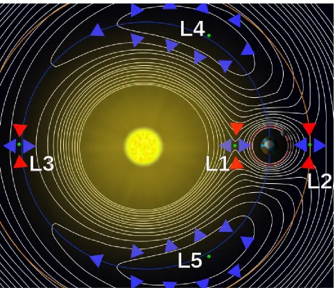
Named after the French-Italian physicist, Joseph Lagrange, the Lagrangian points related to points or regions of equilibrium within a restricted three-body-problem (Carroll & Ostlie 2007). The restriction within this model is that the third body in the system is of comparatively negligible mass, this simplifies the solution considerably. In this model there are a total of five Lagrangian points, their locations are documented in Figure 1.

The simplest way of processing this system is to use an x-y orbital plane with a co-rotating coordinate system, this allows for an essentially immobile system but does require the introduction of two pseudo-forces in the centrifugal and Coriolis forces (Carroll & Ostlie 2007). Under this model each Lagrangian point can be conceived as a point or region of the zero gravitational potential energy. A simple way of deriving this is as per Carroll & Ostlie 2007:

Define the gravitational potential energy (Ug) as:

U_g=−GMm

Where M and m are the masses two bodies, G is the gravitational constant and r the distance between them. From Newtonian physics we know that centrifugal potential energy can be written as:

U_f−U_i=U_c−

∫

rj

ri

Fc⋅dr (2)

Where Fc is the centrifugal force and the subscript 'f' and 'i' as the final and initial energy and distance.

It is known that:

Fc=mω

2

r (3)

With ω being the angular velocity. Therefore the difference in gravitational potential energy can be written as:

Uc=

−1

2 mω

2

r2 (4)

From this we can ascertain the following equation to locate the Lagrangian points in this system:

U=−G

(

s1

+M2m

s2

)

−1

2mω

2_r2

(5)

Where s1 and s2, relate to the distances between the massive bodies and the third insignificant one.

horseshoe orbit1 _{will traverse the L3 as part of it motion, but will not become} locked to that region. Therefore these three points are of little importance to this study (Carroll & Ostlie 2007).

As mentioned earlier, the primary element of the Trojan populations are the L4 and L5 Lagrangian points. Unlike the L1-L3, these region of space are gravitationally stable and capable of hosting dynamically stable objects on a billion year timescale. This is because as a body would shift away from one of these region the change in potential energy would increase the speed of the body causing a Coriolis effect resulting in the body entering an orbit around the Lagrangian point. It is this effect that allows Trojan objects to librate around the planetary Lagrangian points and maintain long-term gravitational stability.

1.7 Keplerian Elements

Named in honour of Johannes Kepler, one of the most important figures in astronomical history, the Keplerian elements are the defining parameters of orbital motion. These elements are used to guide the inertial frame for all orbiting bodies in our Solar system, and are therefore of great importance to this study. Figure 1 displays a graphical depiction of each element in what this study refers to as a, e, i, ω, Ω, M space. Each of these parameters are explained below (Ryden & Peterson 2010; Carroll & Ostlie 2007).

Semi-major axis (a): Probably the most commonly discussed of the six Keplerian elements, the semi-major is defined as half the length of the major-axis of an objects orbital ellipse, with the systems local centre of mass as the focus.

Eccentricity (e): The eccentricity describes the shape of the orbital ellipse, from a perfect circle, at e = 0, to an escape orbit, at e ≥ 1.

Inclination (i): The inclination is the tilt of the orbital plane as compared to a reference frame in respect to the plane of the Solar System.

Argument of periapsis (ω): Describes the angle between the longitude of the ascending node and the point at which the object is at perihelion (its closest approach to the Sun).

Longitude of the ascending node (Ω): The ascending node is the point at which the orbital plane intersects with the reference plane. In this case, the Longitude of the ascending node is an angle from a reference point (typically the first point of Aries) to the ascending node itself.

2. Methodology

2.1 Target Acquisition

The primary aim of this project was to provide classification through detailed analysis of the long-term dynamical stability of every Neptune Trojan known to date. The list of known Trojans was obtained from the Minor Planet Centre's dedicated Neptune Trojans page (2015) on the 8th _{of November 2015}2_{. At that} time, there were a total of eleven Neptune Trojans listed. For these targets, the best-fit orbital solutions were obtained from the Asteroid Dynamics Site (2016). This revealed that one of the listed Trojans, 2012 GX17, was in fact a Trans-Nepunian Object (TNO) that had been misidentified, with a semi-major axis of ~37au as opposed to the ~30au for typical Neptune Trojans. However, this TNO, 2012 GX17, was retained in the sample, because as a known dynamically unstable object it provides a baseline to compare to known Trojans to.

The data used for the dynamical simulations of each target is tabulated in Table 1, including the date relevant epoch data and the date obtained. This is included as the orbital parameters of these objects are constantly under refinement as more observations are obtained.

2.2 Previous Works

As mentioned in Section 1.2 small scale simulations of the first discovered Neptune Trojan (2001 QR322) showed it to be dynamically stable on billion year timescales (Chaing & Lithwick 2005; Brasser et al. 2004; Mazari et al. 2003).

2 The Minor Planet Center’s Neptune Trojans page can be found at

However, more recent work by Horner & Lykawka (2010a) demonstrated that the stability of this object was not quite as simple, and raised questions regarding the stability of other objects in this population.

In addition, the simulations conducted by Horner, et al. (2012a; 2012b; 2010a) on the the long-term stability of the objects 2001 QR322, 2004 KV18, and 2008 LC18 indicated something new about the impact of orbital parameters on a Trojan's stability; that within the a, e, i Ω, ω, M space, only the semi-major axis and the eccentricity had any real impact on the ejection times on a billion year timescale over the 3σ range of the clone population. Based on this precedent the methodology was altered from the typical norm to create a population that spanned 3σ in only semi-major axis and eccentricity. By focusing in on the parameters with the most impact on an object's stability, this study can produce a much higher resolution study in those areas of importance while conserving computing power and time. This has resulted in detailed stability plots of the previously unexplored Trojans and provide a deeper re-examination of the dynamical stability of 2001 QR322, 2004 KV18, and 2008 LC18.

2.3 The M

package

a single fixed time-step which can cause issues when multiple bodies come into close proximity of each other (Chambers 1999).

To handle this issue, and while still taking fullest possible advantage of a symplectic integrator, this study looked to the MERCURY integration package.

MERCURY includes a hybrid symplectic integrator that uses typical symplectic

algorithms for handling the bulk of the computation but slowly hands over to a Bulirsch-Stoer (Stoer & Bulirsch 1980) N-body integrator as multiple objects draw into close proximity of each other. This essentially allows the benefits of the faster computational times and lower errors of the symplectic integrator while allowing a reduction of the time-step, and as a result increase the accuracy, as two bodies near each other. The program does this by separating the Hamiltonian into three parts; HA, HB, and HC (Chambers 1999). The three separated Hamiltonian terms are expressed as follows:

HA=

∑

N

(

2m_i−

Gm_om_i

r_ij

)

H_B=−G

∑

i=1

N

∑

j+i+1

N

(

r_ji

)

HC=

1 2m_o

(

∑

N

pi

)

2

(8)

Where m denotes mass, p denotes momentum G the gravitational constant, r the radius, and i and j refer to the two bodies in question. However this process is only accurate when the bodies are at such a distance that, HA » HB and HA » HC, as the two approach one another, this method is no longer appropriate.

for this, we need to move the rij term from HB to HA. The result is now (Chambers 1999):

H_A=

∑

i=1

N

(

2m_i−

Gm_om_i r_ij

)

G m_am_b

r_ab (9)

HB=−G

∑

N

∑

j+i+1

N

(

r_ji

)

∑

(

r_aj

)

It is worth noting that HA can not be integrated analytically in this form as it contains the three-body-problem. This proves to be a non-issue as it can be integrated numerically to a high level of precision. The final stage is to allow the hand over to happen gradually, and to allow HA » HB. This is achieved by introducing a term K based on (Chambers 1999):

K=

{

0

y2/(2y2−2y+1)

1

for y<0

for0<y<1

for y>1

(11)

where y:

y=

(

0.9r_crit

)

and rcrit is a free parameter. Using this the final form for the Hamiltonian becomes (Chambers 1999):

HA=

∑

N

(

2m_i−

Gm_om_i

r_ij

)

∑

N

∑

j+i+1

N

(

r_ji

)

H_B=−G

∑

i=1

N

∑

j+i+1

N

(

This allows for the gradual hand over from a symplectic integrator to a Bulirsch-Stoer N-body integrator and back again as the two or more bodies move into close proximity of each other and out again.

As stated above, this style of integrator proves invaluable to the type of dynamical simulations used here. The energy errors caused by classical n-body integrators would likely have a negative impact on the subtle nature of the Trojans and introduce significant uncertainly into the validity of the results. This hybrid method provides the best of both worlds, allowing for accurate results with reasonable computational time (Chamber 1999).

2.4 Simulations and Simulation Parameters

The simplest and most effective way to test the long term gravitational stability of the Neptune Trojans is create a cloud of clones existing in the a, e, i, ω, Ω, M space centred on the nominal best fit orbit of a given object, with the cloud radiating out to 3σ in each of the six orbital dimensions. As discussed in section 2.2, it is known from previous works (Horner et al 2012a, 2012b, 2010a) that the majority of these orbital elements, barring the eccentricity and the semi-major axis, have little impact on the long-term dynamical stability of the Trojans.

parameters that typically cause instability while reducing the required computational times by cutting the overall number of test particles down by almost a third compared to the works of Horner et al (2010a).

To simulate each Neptune Trojan in turn the MERCURY dynamics package was set

up with the Sun as the central body, and each of the 4 major Jovian planets (Jupiter, Saturn, Uranus, and Neptune)3_{. It is worth noting that as part of these} simulations we do not include other Solar system bodies such as the terrestrial planets or any objects from the Asteroid belt, Kuiper belt or Oort Cloud populations, as is standard procedure in this field of work (Horner & Lykawka 2012b). Any of these objects would have little to no effect of the long stability of the of the test particles, but they could severely complicate the systems and massively increase the computational times of each simulation.

The ejection radius was set to be 1000au4 _{from the centre of the Solar system.} From here each cloud of 6,561 clones was entered into the package to simulate their movement under the gravitational influence of these five massive bodies. The integration time-step for MERCURY was set to 100 days

while the write out time step was set to every 100,000 years, recording the status of the test particles. Any object that either collided with the Sun, one of the Jovian planets, or exceeded the ejection radius was removed from the system, and this event recorded. Table 1 list the Kelperian elements of each Trojan used in these simulations alongside the date these elements were obtained.

3 The full planetary elements used for the simulations can found in Appendix 1 4 The 1000au ejection distance represents a first order approximation between the

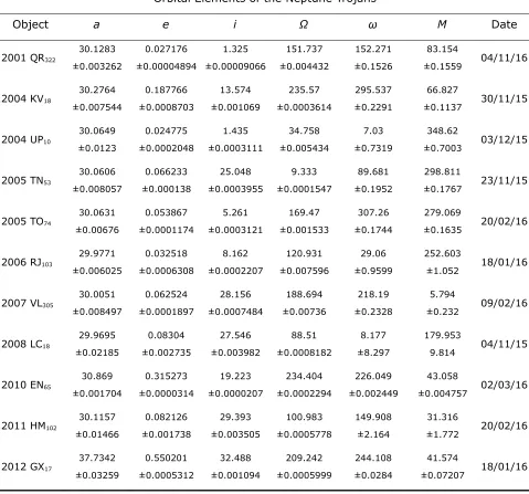
Table 1: The Keplerian elements of each Neptune Trojan, with the 1σ errors recorded below each value. Additionally, we have included that date that the variables were obtained as these update frequently. All data taken from the Asteroids Dynamics Site (2016). All parameters are barycentric with a JD2000 reference point.

Orbital Elements of the Neptune Trojans

Object a e i Ω ω M Date

2001 QR322 30.1283

±0.003262 0.027176 ±0.00004894 1.325 ±0.00009066 151.737 ±0.004432 152.271 ±0.1526 83.154 ±0.1559 04/11/16

2004 KV18 30.2764

±0.007544 0.187766 ±0.0008703 13.574 ±0.001069 235.57 ±0.0003614 295.537 ±0.2291 66.827 ±0.1137 30/11/15

2004 UP10 30.0649

±0.0123 0.024775 ±0.0002048 1.435 ±0.0003111 34.758 ±0.005434 7.03 ±0.7319 348.62 ±0.7003 03/12/15

2005 TN53 30.0606

±0.008057 0.066233 ±0.000138 25.048 ±0.0003955 9.333 ±0.0001547 89.681 ±0.1952 298.811 ±0.1767 23/11/15

2005 TO74 30.0631

±0.00676 0.053867 ±0.0001174 5.261 ±0.0003121 169.47 ±0.001533 307.26 ±0.1744 279.069 ±0.1635 20/02/16

2006 RJ103 29.9771

±0.006025 0.032518 ±0.0006308 8.162 ±0.0002207 120.931 ±0.007596 29.06 ±0.9599 252.603 ±1.052 18/01/16

2007 VL305 30.0051

±0.008497 0.062524 ±0.0001897 28.156 ±0.0007484 188.694 ±0.00736 218.19 ±0.2328 5.794 ±0.232 09/02/16

2008 LC18 29.9695

±0.02185 0.08304 ±0.002735 27.546 ±0.003982 88.51 ±0.0008182 8.177 ±8.297 179.953 9.814 04/11/15

2010 EN65 30.869

±0.001704 0.315273 ±0.0000314 19.223 ±0.0000207 234.404 ±0.0002294 226.049 ±0.002449 43.058 ±0.004757 02/03/16

2011 HM102 30.1157

±0.01466 0.082126 ±0.001738 29.393 ±0.003505 100.983 ±0.0005778 149.908 ±2.164 31.316 ±1.772 20/02/16

2012 GX17 37.7342

±0.03259 0.550201 ±0.0005312 32.488 ±0.001094 209.242 ±0.0005999 244.108 ±0.0284 41.574 ±0.07207 18/01/16

2.5 Stability Analysis

orbital elements, a technique that has been widely used in the field (e.g. Horner et al 2004a,b, 2010a, 2012a, Wittenmyer et al. 2016). From this we can gain an important insight into the long term gravitational stability of each object, and thus be able to correctly characterise them as primordial, captured or boundary case.

The MERCURY simulations track the time at which each of the cloned test

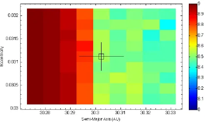
particles are ejected from the Solar system or collides with another body. This output can be used to create files detailing the ejection times of each test particle, with an ejection time of 4 Gyrs used for those that remain in the system (for the purpose of visualising the data). This allows for the creation of stability maps, the established norm of this field of work (Wittenmyer et al. 2016; Horner & Lykawka 2012ab), by plotting the ejection times as a colour map in an eccentricity VS semi-major axis space. An example of such a map, from Horner et al (2012b), can be seen in Figure 3.

Figure 3 shows the stability map for 2008 LC18, the plot clearly demonstrates any relationship between the orbital parameters of the Trojan and it's lifetime. From this it is a trivial matter to determine the classification of each object and to gain a clear understanding of its long term gravitational evolution.

2.6 Libration Simulations

A secondary research component of this study was to investigate the nature of each Trojans' initial libration, and to see if there was any correlation with the object's long-term stability. Of particular interest to this project were the amplitudes and period of librations while the object trapped around either the L4 or L5 Lagrangian points.

To best archive this goal, once again the MERCURY dynamics package was used

to simulate a swarm of clones for each Trojan using the same a, e, i, ω, Ω, M

space and 81x81 arrays used to populate the stability simulations and track their resonant angle in relation to Neptune.

at the initial point of the object's the orbital solution. This allows for the timescale of the simulations to be brought down to just 100,000 years. This still provides important and detailed information on the initial behaviour of Trojans around the L4 and L5 Lagrangian points, but brings the storage and computational time down to a manageable amount.

2.7 Analysing the Libration

The libration amplitude and periods of each clone are, in theory, very easy compute as this study is simply trying to detect any periodic behaviour in the resonant angle of the object.

As found from the nature of the librations seen in the Jupiter Trojans by Jewitt et al. (2000) and Shoemaker et al. (1997), one would expect the Neptune Trojans to exhibit similar periodic behaviour but on a much longer time scale given the significantly longer orbital period of Neptune. While the preliminary data does support this hypothesis, early analysis of 2008 KV18 demonstrated a tendency for members of the clone swarm to change orbital states ranging from entering into horseshoe orbits to switching from leading to trailing Lagrangian points and vice versa. While this proved a fascinating development and hints at significantly higher system complexity than originally anticipated, it did complicate the normal, and planned, methodology of running a standard periodogram. Given this complicated nature of the Trojan behaviour a new method for the analysis would need to be found.

3. Results and Discussion

To clearly discuss the results of each Neptune Trojan the analysis is broken down into three distinctive areas. The first will focus on the classification of each object based on the results of the stability mapping and discuss any correlation between ejections times and any objects initial eccentricity or semi-major axis parameters. The second section will delve into the rate of decay of the unstable simulated swarms to give an insight into the nature of the objects. The final section will discuss results of the libration angle and/or amplitude of the each test particle during the initial simulation stages to investigate whether there is any correlation between these initial parameters and the long-term dynamical stability of each object.

3.1 Analysing the Stability Maps

As discussed in the methodology the primary way of analysing a Trojans long-term dynamical stability and accurately classifying the object is to study the stability maps created from the ejection files of each Trojans' simulation. For the sake of brevity and to prevent unnecessary repetition, each object will be discussed under on the following classifications:

• Captured: Complete Instability • Primordial: No Ejections

• Primordial: Limited Ejections • Primordial: Borderline Instability • The Trans-Neptunian Object

3.1.1 Captured: Complete Instability

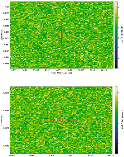
Figure 4: The two Neptune Trojans 2004 KV18 (top) and 2010 EN65 (bottom) as a functions of

Neptune Trojans 2008 KV18 and 2010 EN65 displayed text-book examples of the behaviour, as demonstrated in Figure 4. Both objects show near identical chaotic behaviour with the majority of test particles ejected from the Solar system on approximately 10 Myr timescales, behaviour similar to that of a Centaur (Pal et al 2015; Horner et al 2004ab). Both of these objects can be clearly classified as temporarily captured Trojans. As can be seen in both figures there is quite a lot of variation in the ejections of the test particles, with some escaping only a few hundreds of thousands of years into the simulation while a small subset even managed to survive the full 4 Gyrs. Of the 6561 clones in the individual swarms only 24 and 21 test particles (for 2008KV18 and 2010EN65 respectively) remained in the system after the 4Gyr simulation. It is also worth noting that while these test particles may have remained in the system none of them where still in Trojan orbits. This demonstrates the chaotic nature of such objects and reinforces the validity of the “swarm” method used.

For 2008 KV18, these maps support earlier studies by Horner et al (2012a), which also classified the object as captured. It is reassuring to note that both studies came to same conclusion (with similar ejection times), even with the increased resolution and orbital solution accuracy.

3.1.2 Primordial: No Ejections

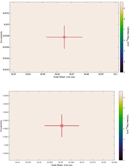
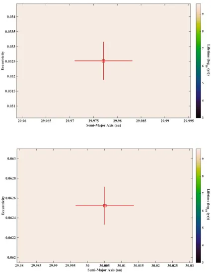
Figure 5: The Neptune Trojans 2004 UP10 (top) and 2005 TN53 (bottom) as a function of

Figure 6: The Neptune Trojans 2006 RJ103 (top) and 2007 VL305 (bottom) as a function of

3.1.3 Primordial: Limited Ejections

As can be seen in the stability maps of 2005 TO74, and 2011 HM102 in Figure 7 these objects demonstrate very few ejections over the 4 Gyr lifetimes. Despite the few ejected test particles these maps still indicate high level stability, and that both Trojans are most likely Primordial in nature. It is not unexpected for Primordial Trojans to undergo a small amount of attrition within the test swarm even in the most stable regions. As can be seen in both maps, even the clones removed from the system still displaying long-term orbital stability with all particles still demonstrating stability on a billion year timescale even if they do not quite survive the full simulation. Interestingly, while both clouds suffer from a small amount of attrition in their respective population they are different in nature. While 2005 TO74 displays largely chaotic and well distributed ejections, 2011 HM102 shows a stronger ejection rates in the upper left-hand corner. This hints a possible increase in the instability of the region as the as the eccentricity and semi-major axis increase. Regardless of this minor number of ejections both Neptune Trojans 2005 TO74 and 2011 HM102 are primordial objects, however they do demonstrate small amount of dynamical instability on the Gyr timescale.

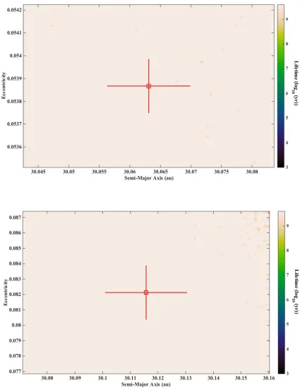
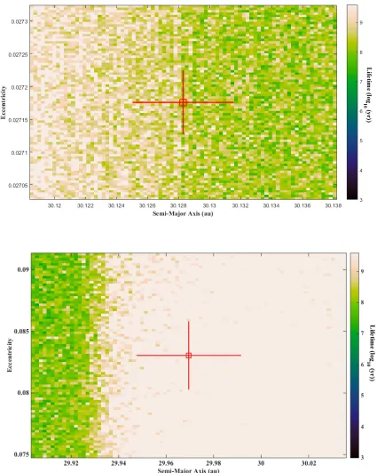
3.1.4 Primordial: Borderline Stability

Figure 7: The Neptune Trojans 2005 TO74 (top) 2011 HM102 (bottom) as a function of

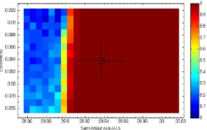
Figure 8: The Neptune Trojans 2001 QR322 (top) and 2008 LC18 (bottom) as a function of

Eccentricity and Semi-major Axis over a range of 3σ. The red central square relates to the original orbital parameters at epoch, with the lines projecting from the centre displaying ±1σ. Each square in the plot relates to one of the 81x81 clones used to populate the a x e space in the simulations. Note for both objects there are two distinct regions of stability dependant on the semi-major axis. For 2001 QR322 there is a clear border of stability at ~30.128au, with the

region outward of that boundary displaying massive instability on a 10Myr timescale. While with 2008 LC18 the region exceeding ~29.94au demonstrates a longer dynamically stable

the semi-major axis, with 2001 QR322 becoming unstable when a > 30.128au, and demonstrating the same instability in 2008 LC18 when a < 29.94au. This is caused by each object being located on the edge of their respective stable regions, as such a fast attrition of test particles can be seen in the region that exceed this boundary. Both of these Neptune Trojans are likely primordial in nature, however are probably part of what would have been a much larger population of Trojans in that area during the early stages of the Solar system.

3.1.5 The Trans-Neptunian Object

Finally, there was the black sheep of the test sample, 2012 GX17. As mentioned previously 2012 GX17 was misidentified as a Neptune Trojan but when the

Figure 9: 2012 GX17 as a function of Eccentricity and Semi-major Axis over a range of 3σ. The

red central square relates to the original orbital parameters at epoch, with the lines projecting from the centre displaying ±1σ. Each square in the plot relates to one of the 81x81 clones used to populate the a x e space in the simulations. 2012 GX17 was identified as a potential

orbital solution for the object was refined it was clear the object was trans-Neptunian in nature, with a semi-major axis exceeding ~37au. As can been in Figure 9 the object is entirely unstable on a 10 Myr timescale, similar to that of the captured Trojans. This behaviour was expected but does also provide a baseline of sorts for comparison. It is worth noting that, from the objects stability maps, that it does appear to be stable on a slightly longer time scale then 2008 KV18 and 2010 EN65. After some discussion and consideration, we conclude that the cause was most likely due to the increased orbital period of the object. As a follow on from this, we are planning to investigate this further, the finding of which is to be included in future publications.

3.2 Decay of the Unstable Trojans

Having addressed the stability maps of all ten Trojans, the singleton TNO, and classified each object accordingly, it is worth investigating the decay of the clones of each individual Trojan identified as unstable or borderline stable. This section will discuss the attrition rates of the each dynamically unstable Trojan cloud by classification.

3.2.1 Captured Trojans and 2012 GX17

Figures 10, through to 12 display the decay of the two captured Trojans, 2004 KV18 and 2010 EN65, and the Trans-Neptunian Object, 2012 GX17. The first thing that is immediately apparent is that all three objects have very similar features in their decay plots, with 2004 KV18 and 2010 EN65 being almost identical. In the case of all three display a period of initial stability on a million timescale as the swarm of clones disperse, followed by a lengthy period of decay.

entirety of the 4Gyr simulation, with 24 and 21 survivors for 2004 KV18 and 2010 EN65 respectively. This data reinforces the earlier classifications that both objects are temporarily captured Trojans that demonstrate behaviour that is dynamically unstable on a billion year timescale. This also supports earlier simulations in regards to the decay of 2004 KV18 by Horner & Lykawka (2012a).

Similar behaviour witnessed in the TNO 2012 GX17 but with slightly longer period of initial stability. The TNO does not begin to enter into its attrition phase for about five million years. While this does delay its inevitable decay the final result remains the same, with only 19 of the 6,561 test particles surviving the full 4Gyrs. This may be an indication that the object is a temporary capture to the 3:2 mean-motion resonance of Neptune – temporary Plutino, although further study would be required to confirm this.

3.2.2 Borderline Primordials

The previous section categorised both 2001 QR322 and 2008 LC18 as dynamically stable objects that reside on the outer boundary of the gravitationally stable Lagrangian points. This classification is supported in the attrition of the test particles for both objects. As can be clearly seen from Figures 13 and 14, that both populations of clones are completely stable on 10Myrs timescale. After this initial periods of stability the outer edge of the cloud begins to decay overtime in a similar nature to the above captured Trojans. In the case of the both objects a significant proportion of the test particles survive the simulation, 968 for 2001 QR322 and 4,557 for 2008 LC18.

Figure 10: Displayed is the attrition of the 2004 KV18's test particles as a function of Log(time)

Figure 11: Displayed is the attrition of the 2010 EN65's test particles as a function of Log(time)

and either the number of particles remaining (top) or of Log(number of particles remaining). 2010 EN65 demonstrates remarkably similar rate of decay to 2004 KV18. With an initial period

Figure 13: As seen from the stability maps, the swarm of test particles used for the 2001 QR322

Lagrangian points would begin to decay after tens of millions of years, with almost the entire outer section of Trojans eroding away over our 4 Gyr lifetime. This support both our earlier stability data and the results of earlier decay simulations into these objects. (Horner & Lykawka 2012b; Horner & Lykawka 2010)

3.3 Impact of Libration Amplitude and Period

Unfortunately due to an accelerated timeline, we were unable to complete and process the libration data from our simulations before the writing of this manuscript. However this section will present some preliminary data from the captured Neptune Trojan, 2004 KV18. Figures 15 and 16 demonstrate just some fascinating behaviour seen on a much shorter timescale than initial anticipated.

Figure 15 displays typical behaviour for a tadpole orbit that one would expect to see over the 100,000 year timescale of both Primordial and Captured Trojans, however it is worth noting that the libration period of this test particle does increase with time, possibly hinting at early instability. However, very few of the test particles demonstrate this behaviour, with many evolving to different orbits or becoming ejected Lagrangian points entirely. Figure 15 also displays one of our test particles exiting from its current tadpole orbit in the L4 and jumping into another in the L5 via the L3, behaviour that would classify the object as a Jumping Trojan. A typical horseshoe orbit can be seen in Figure 16, as the object rapidly (on the order of 60,000 years) moves from the initial tadpole orbit into a classical Horseshoe orbit, alas the timescale of the of the simulations is not long enough to witness whether the test particle re-stabilises into a tadpole, continues on in as a horseshoe, or escapes the system.

exhibited the behaviour witnessed in the lower panel of Figure 16. As can be seen the clone exits the 1:1 mean-motion resonance at around the 60,000 year mark (a recurring point for all of the preliminary data on 2004 KV18) and enters into either the Centaur or TNO population (Horner & Lykawka 2010b). However the object is re-captured into the L5 after just ~10,000 years and continues on in a tadpole orbit. Given the ejection times from 2004 KV18 clone swarm, it would appear that recapture early in the objects evolution was very possible, and likely the norm for this population of clones. However, it is once again worth noting that our simulation only removes an object when it either collides with another body or leaves the Solar system entirely, and this will result it a certain delay between ejection from the stable Lagrangian point regions and removal from our simulation.

4. Conclusion

Through the use of computational simulations this study have been able to analyse the stability of each of Neptune's known Trojan asteroids and classify the likely timescales in which the objects have been hosted by Neptune. It was found the Trojans 2004 UP10,2005 TN53, 2006 RJ103, 2007 VL203, 2005 TO74, and 2011 HM102 to be dynamically stable on the Solar system's 4 Gyr timescale and therefore primordial in nature. The objects 2001QR322 and 2008 LC18, are also likely primordial in nature, but both exist just on the cusp Neptune's stable regions, and were therefore probably a part of a large population of Trojan asteroids captured during Neptune's final stages of planetary migration. Finally the study found only two of the ten Neptune Trojans to be completely dynamically unstable on a billion timescale; 2004 KV18, and 2010 EN65. These objects are almost certainly recent captures of Neptune with neither object being stable beyond tens of millions of years.

Future Works and Publications

While the research already completed has allowed for a deep insight into the nature of ten of the known Neptune Trojans and allowed for their individual classification, there is plenty of room for additional research.

There are two particular areas of interest to the author. Firstly, we will need to expand the simulations already completed to include the newly confirmed and discovered objects announced in September of this year (Lin et al. 2016) to provide stability maps and classification of these new objects. Finally we will complete the investigation into the impact of libration amplitudes and periods on the overall long-term dynamical stability of the Neptune Trojans (including the newly announced Trojans). As part of this, we will investigate the nature of the librations themselves. To do this, we will run two separate sets of simulations; short timescale, high-resolution simulation to ascertain the initial conditions in relation to the overall lifetime, and another set of simulations run on a billion year timescale with a severely reduced resolution in both time and

a, e space to allow for reasonable computational times.

References

Asteroids Dynamics Site 2016, European Space Agency, 04/11/2015 <http://hamilton.dm.unipi.it/astdys/>.

Brasser, R, Mikkola, S, Haung, TY, Wiegert P, Innanen, K 2004, 'Long-term evolution of the Neptune Trojan 2001 QR322', Monthly Notices of the Astronomical Society, 347, 833-836

Carroll, BW & Ostlie, DA 2007, An Introduction to Modern Astrophysics, 2nd edn, Pearson, San Francisco.

Chaing, EI &, Lithwick, Y 2005, 'Neptune Trojans as a test bed for planetary formation', The Astronomical Journal, 628, 520-532.

Chambers, JE 1999, 'A hybrid symplectic integrator that permits close encounters between massive bodies', Monthly Notices of the Royal Astronomical Society, 304, 793-799.

Emery, JP, Marzari, F, Mordibelli, A, French, LM, Grav, T 2015, 'The Complex History of Trojan Asteroids', Asteroids IV, 203-221.

Fernandez, JA & Ip, WH 1996, 'Orbital Expansion and resonant trapping during the late accretion stages of the outer planets', Planetary Space Science, 44, 431-440.

Fleming, HJ & Hamilton, DP 2000, 'On the origin of the Trojan asteroids: Effects of Jupiter’s mass accretion and radial migration', Icarus, 148, 479-493.

Society, 354, 798-810.

Horner, J, Evans, NW, Bailey, ME 2004, 'Simulations of the population of Centaurs – II. Individual objects', Monthly Notices of the Royal Astronomical Society, 355, 321-329.

Horner, J, Lykawka, PS 2010, '2001 QR322: a dynamically unstable Neptune Trojan?', Monthly Notices of the Royal Astronomical Society, 405, 49-56.

Horner, J, Lykawka, PS 2010, 'The Neptune Trojans – a new source of the Centaurs', Monthly Notices of the Royal Astronomical Society, 402, 13-20.

Horner, J, Lykawka, PS 2010, 'Planetary Trojans – the main source of short period comets?', International Journal of Astrobiology, 9, 227-234.

Horner, J, Lykawka, PS 2012, '2004 KV18: a vistor from the scattered disc of the Neptune Trojan population', Monthly Notices of the Royal Astronomical Society, 426, 159-166.

Horner, J, Lykawka, PS 2012, 'Are Two of the Neptune Trojans Dynamically Unstable?', The Australian Space Research Conference Proceedings, 11.

Horner, J, Lykawka, PS, Bannister, MT, Francis, P 2012, '2008 LC18: a potentially unstable Neptune Trojan', Monthly Notices of the Royal Astronomical Society, 422, 2147-2151.

Horner, J, Gilmore, JB, Waltham, D 2014, 'The role of Jupiter in driving Earth's orbital evolution: An update', The Australian Space Research Conference Proceedings, 14.

Kortenkamp, SJ, Malhotra, R, Michtchenko, T 2004, Survival of the Trojan-type companions of Neptune during primordial planet migration', Icarus, 167, 347-359.

Lin, HW, Chen, YT, Holman, MJ, Ip, WH, Payne, MJ, Lacerda, P, Fraser, WC, Gerdes, DW, Bieryla, A, Sie, ZF, Chen, WP, Burgett, WS, Denneau, L, Jedicke, R, Kaiser, N, Magnier, EA, Torny, JL, Wainscoat, RJ, Waters, C 2016, 'The PAN-STARRS 1 Discoveries of five new Neptune Trojans', The Astronomical Journal, 152, 147-155.

Lykawka, PS, Horner, J, Jones, BW, Mukai, T 2009, 'Origin and dynamical evoltuon of Neptune Trojans – I. Formation and planetary migration', Monthly Notices of the Royal Astronomical Society, 398, 1715-1729.

Lykawka, PS, Horner, J 2010, 'The capture of Trojan asteroids by the giant planets during planetary formation, Monthly Notices of the Royal Astronomical Society, 405, 1375-1383.

Lykawka, PS, Horner, J, Jones, BW, Mukai, T 2010, 'Formation and dynamical evolution of the Neptune Trojans – the influence of the initial Solar system architecture', Monthly Notices of the Royal Astronomical Society, 404, 1272-1280.

Lykawka, PS, Horner, J 2011, 'The Capture and release of Trojan asteroids by the giant planets during the solar system history', EPSC Abstracts, 6, 1264-1265.

Lykawka, PS, Horner, J, Mueller, T 2013, 'On the orbital (in)stability of Trojan asteroids in the solar system', Spaceguard Research, 5, 13-16.

de la Fuente Marcos, C & de la Fuente Marcos, R 2014, 'Asteroid 2013 ND15: Trojan companion to Venus, PHA to the Earth', Monthly Notices of the Royal Astronomical Society, 443, L59-L63.

Malhotra, R 1995, 'The origin of Pluto's orbit: Implications for the solar system beyond Neptune', The Astronomical Journal, 110, 1.

Marzari, F, Tricarico, P, Scholl, H 2003, 'The MATROS project: Stability of Uranus and Neptune Trojans. The case of 2001 QR322', Astronomy & Astrophysics, 410, 725-734.

Marzari, F, Scholl, H 2013, 'Long term stability of Earth Trojans', Celestial Mechanics and Dynamical Astronomy, 1, 91-100.

Morbidelli, A, Levison, HF, Tsiganis, K, Gomes, R 2005, 'Chaotic capture of Jupiter's Trojan asteroids in the early Solar system', Nature, 435, 462- 465.

Nicholson, SB 1961, 'The Trojan Asteroids', Astronomical Society of the Pacific, 381.

Pal, A, Kiss, CS, Horner, J, Szakats, R, Vilenius, E, Muller, TG, Acosta-Pulido, J, Licandro, J, Cabrera-Lavers, A, Sarneczky, K, Szabo, GM, Thirouin, A, Sipocz, B, Dozsa, A, Diffard, R 2015, 'Physical properties of the extreme Centaur and super-comet candidate 2013AZ60', Astronomy and Astrophysics, 583, A93.

Ryden, B & Peterson, BM 2010, Foundations of Astrophysics, Pearson, San Francisco.

Scholl, H, Marzari, P, Tricarico, P 2005, 'Dynamics of Mars Trojans', Icarus, 175, 397-408.

Sheppard, SS & Trujillo, CA 2006, 'A Think Cloud of Neptune Trojans and Their Colours', Science, 313, 511-514.

Shoemaker, EM, Shoemaker, CS, Wolfe, RF 1997 Asteroids II, R.P Binzel, T. Gehrels & M.S. Matthews, University of Arizona Press, 487.

Stoer J & Bulirsch, R 1980, Introduction to Numerical Analysis, Springer-Verlag, New York

The Minor Planet Center 2015, The International Astronomical Union, 04/11/2015, <http://www.minorplanetcenter.net/>.

Wittenmyer, RA, Horner, J, Mengel, MW, Butler, RP, Tinney, CG, Carter, BD, Wright, DJ, Jones, HRA, Bailey, J, O'Toole, SJ 2016, 'The Anlgo-Australian Planet Search XXV: A Candidate Massive Saturn Analog, Orbiting HD30177,

Monthly Notices of the Royal Astronomical Society, submitted.

Appendix 1

Table 2: The Orbital elements of the four gaint planets as used in the MERCURY code for the Neptune Trojan simulations,

down to five significant figures; these are vaild at epoch JD 2457400.

Obrital elements on the four giant planets used in the MERCURY simulations

Jupiter Saturn Uranus Neptune

Mass (Mo) 9.5479x10-4 _2.8588x10-4 _4.3662x10-5 _5.1514x10-5

Density 1.33 0.7 1.3 1.76

Cartesian x 4.8414 8.3434 1.2894x101 _1.5380x101

Cartesian y -1.1603 4.1248 -1.5111x101 _-2.5919x101

Cartesian z -1.0362x10-1 _-4.0352x10-1 _-2.2331x10-1 _1.7926x10-1

Velocity x (au/day) 1.6601x10-3 _-2.7674x10-3 _2.9646x10-3 _2.6807x10-3

Velocity y (au/day) 7.6990x10-3 _4.9985x10-3 _2.3784x10-3 _1.6282x10-3