Validation of a community district energy system model using field measured data
Behrang Talebi, Fariborz Haghighat, Paul Tuohy, Parham Mirzaie
PII: S0360-5442(17)32087-X DOI: 10.1016/j.energy.2017.12.054 Reference: EGY 12003
To appear in: Energy
Received Date: 27 August 2017 Revised Date: 2 December 2017 Accepted Date: 11 December 2017
Please cite this article as: Talebi B, Haghighat F, Tuohy P, Mirzaie P, Validation of a community district energy system model using field measured data, Energy (2018), doi: 10.1016/j.energy.2017.12.054.
M
AN
US
CR
IP
T
AC
CE
PT
ED
Validation of a Community District Energy System Model Using Field Measured Data
1 2
Behrang Talebi1, Fariborz Haghighat1*, Paul Tuohy2, Parham Mirzaie3
3
1
Department of Building, Civil and Environmental Engineering, Montreal, Canada
4
2
Mechanical and Aerospace Engineering, University of Strathclyde, Glasgow
5
3
Architecture and Built Environment Department, The University of Nottingham, Nottingham,
6
UK
7 8
ABSTRACT
9
Load prediction is the first step in designing an efficient community district heating system
10
(CDHS). Even though, several methods have been developed to predict the heating demand
11
profile of buildings, there is a lack of method that can predict this profile for a large-scale
12
community with a numerous user types in a timely manner and with an appropriate level of
13
precision.
14
It, first briefly describes the 4-step procedure developed earlier, utilizing a Multiple Non-Linear
15
Regression (MNLR) method, for predicting the heating demand profile of district, followed by
16
description of the community structure, and its district system. It also reports the field
17
measurement procedure for collecting the data required and the preliminary analysis data.
18
Results obtained from a continuous monitoring of the CDHS over a two-year period is employed
19
to validate the accuracy of the developed model in the predicting the CDHS’s heating load
20
profile. Finally, using the 4-step procedure, the district’s energy demand profile is predicted, and
21
compared with both the measured data and the initial prediction. The outcome shows a less than
22
11.2% in the mean square root error (MSRE) of the predicted and measured load profiles.
23
24
Keywords: Load Prediction, District heating System, Validation, Clustering
25
26
27 28 29
*
Corresponding Author: [email protected]
M
AN
US
CR
IP
T
AC
CE
PT
ED
1. Introduction
31
Providing secure and clean source of energy to respond the households’ demand is one of
32
the upmost fundamental challenges faced by the energy planners. In effect, households represent
33
a significant share of the total energy demand; they are responsible for 40% and 26% of the total
34
energy consumption in North America and Europe, respectively [1]. In the last few decades,
35
using fossil fuels as the world's main energy source has resulted in their depletion and increased
36
the level of CO2 equivalent emissions. There are targets for reductions in CO2 emissions
37
worldwide. Specifically, the Energy Technology Perspective 2012 Roadmap (IEA) aims to
38
reduce CO2 emissions by 50% [2]. Given the expected rise in household energy consumption, the
39
building sector is now required to adapt to the new ambitious demands of developing Net-Zero
40
Energy Buildings/communities (NZEB) by 2050.
41
Numerous building energy conservation strategies have been tested using energy storage
42
[3-5] and user-demand [6] methods. The Hybrid Community-District Heating System (H-CDHS)
43
is a unique energy management alternative given its storage and renewable systems are
44
integrated in the district’s thermal energy system. Since the energy generated by renewable
45
sources is not uniform throughout the day, a thermal energy storage unit allows the system to
46
synchronize with the supply and demand. To implement this system effectively, it is essential to
47
predict the H-CDHS’ detailed energy demand profile[7].
48
Hence, several methods have been developed to model buildings’ energy demand profile
49
[8-10]. Given its restricted number of users, a small-scale Hybrid Community District Heating
50
System (H-CDHS) energy demand profile can be predicted using a detailed model of users’
51
consumption created with energy simulation models [8]. Conversely, in large district scale
52
systems, due to the large volume of users, a comprehensive modeling is time-consuming,
M
AN
US
CR
IP
T
AC
CE
PT
ED
computationally expensive and sometimes impractical. Some researchers used comprehensive
54
models to predict the heating demand profile of larger scale communities [11, 12]. To overcome
55
this problem, variety of simplified models were developed to predict the heating demand profile
56
or total energy demand of large communities. These simplified models could be divided into four
57
major categories—black box models (e.g. ANN) [13]; gray box models [14, 15]; equivalent RC
58
networks [16-18]; and regression models [19-24]. Regardless of the method chosen, previous
59
demand estimates focused mainly on predicting the peak and total energy demand. Only few
60
studies tried predicting the demand profile [11, 14, 23].
61
Though these simplified models could reduce the computational time to a fraction of that
62
of comprehensive models, their simplicity would compromise the prediction accuracy due to
63
limitation of the simplified models. Three major drawbacks could be assumed for most of these
64
simplified modes. First, the low prediction accuracy emerging from assumptions made in
65
modeling the individual buildings/units a) presentation of the occupants’ behaviour and, b) the
66
interaction of each building with surrounding buildings in an urban setting. One of the most
67
challenging issues of heating demand prediction models is having to correct input parameters.
68
Input parameters that are dependent on occupants’ behaviour/activities, including heating set
69
points and schedules; Internal heat gain due to occupants’ activity and the building’s heating
70
system; natural ventilation flow rate; solar gains from using windows blinds or shades, etc.
71
Second, scaling effects impair accuracy by oversimplifying scaling methods that extrapolate
72
results from building level to the district level. And third, flexible methods that predict
73
community load profile in diverse building types. More details regarding the limitation of
74
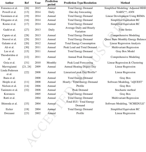
previous projects can be found in previous works done by authors [8, 25]. Table 1 summarizes
75
studies related to CDHS’ heat demand prediction. A closer analysis of existing models reveals
M
AN
US
CR
IP
T
AC
CE
PT
ED
that the current scholarship requires further validation of models that predict heating demands
77
using measured data.
78
This paper endorses a 4-step procedure developed to predict the energy demand profile
79
for H-CDHS. It, first briefly describes the 4-step procedure [25] developed earlier for predicting
80
the heating demand profile of district, followed by description of the community structure, and
81
its district system. It also reports the field measurement procedure for collecting the data required
82
for validating the model from the West Whitlawburn Housing Co-Operative (WWH) CDHS in
83
Scotland. The measurement technique, and the preliminary analysis data are explained. Finally,
84
using the 4-step procedure, the district’s energy demand profile is predicted, and compared with
85
both the measured data and the initial prediction.
86
87
Table 1: Load Prediction Summary
88
89
2. Methodology
90
2.1. The four-step demand profile procedure
91
Talebi et al [25] developed a simplified model to predict the heating demand profile and peak
92
loads in complex district systems Figure 1 shows the procedure used in the development of the
93
simplified models. The procedures are based on the Multiple Linear Regression (MLR) and
94
Multiple Non-Linear Regression (MNLR) methods. In this four-step procedure, the entire
95
district’s heating demand profile is predicted by modeling each individual unit in the community
96
using its physical and geometrical characteristics, the regions’ meteorological information, and
97
the occupants’ general behavior.
M
AN
US
CR
IP
T
AC
CE
PT
ED
1) In the first step, a sample building stock model (BSM) is segmented into different archetypes, and 99
a reference building is defined for each archetype. The initial segmentation is completed by considering 100
the building’s construction method, physical and geometrical properties, and construction period [25]. 101
Once the initial archetypes are determined, each archetype is further divided into sub-archetypes based on 102
the occupancy schedule (e.g. residential user with high, medium and low usage, etc.) of the building 103
within that archetype. Different methods are used for segmenting the BSM based on the occupancy 104
schedule. While some researchers only segment the BSM based on major occupancy types (e.g. 105
residential, commercial, or office types), others segment it following the user’s energy profile. This study 106
presents a more detailed approach for defining the number of archetypes as well as the reference building 107
for each archetype. A hierarchical clustering method was adopted for this end. In this method, the data set 108
is split into a prefixed number of clusters. The building closest to the centroid of that cluster is defined as 109
a reference building for that cluster. To define the number of clusters required for a given data set, 110
prefixed number of clusters, the optimal number of cluster is defined using the elbow method. 111
2) The second step involves building the model’s input files. These files are constructed
112
based on the physical properties of individual units, regional meteorological data, and occupants’
113
behaviour. Four different input files were constructed for this study.
114
i) The first input file is the solar dependent variable. This variable is determined using the
115
weather station closest to the district site and defines each unit’s envelope assembly solar heat
116
gain. The solar components obtained from the weather file are translated on each envelope
117
assembly using the incident angle, orientation, and albedo of that assembly.
118
ii) The second input file is the thermal dependent file. The thermal dependent file defined
119
based on the average heat transfer from the unit’s exterior facade, considering its average
120
thermal resistance of the exterior façade of the unit and the indoor-outdoor temperature
121
difference.
M
AN
US
CR
IP
T
AC
CE
PT
ED
iii) The third input file is the units’ internal gain. Should specific data about units’ internal
123
heat generation be unavailable, the general households’ average heat generation can be used.
124
iv) And finally, the fourth input file constructed based on the daily HVAC system on/off
125
cycles.
126
3) In the third step, a reference building’s heating demand profile is initially defined using
127
the data obtained from the measured data. An ANN model is then trained and tested using the
128
reference building’s input file as well as the heating profile of them to obtain the regression
129
coefficients. More detail information regarding the training of the model using the ANN method
130
could be find in [25].
131
4) Finally, in the fourth step, once the MNLR model is trained separately for each
132
archetype, using the reference building, each individual unit’s heating demand profile is
133
predicted by adopting the input file of them [25].
134
135
Figure 1: Simplified procedure to predict the heating demand profile
136
137
3. Description of the community district heating system design
138
The selected Hybrid Community-District Heating System (H-CDHS) is a mid-size
139
community district heating system in Whitlawburn, Cambuslang, Scotland. The WWH was
140
established in 1989 to provide local community control and promote affordable quality housings
141
for lower income families. The community consists of 640+ dwelling units with four types of
142
buildings. Until 2007, all buildings used the conventional individual dwelling electrical heating
143
systems for the space heating and domestic hot water (DHW) supply. In 2007, the administration
M
AN
US
CR
IP
T
AC
CE
PT
ED
board developed their own district heating system to give the community a more affordable
145
energy and improve the quality of indoor environment by increasing energy efficiency and
146
decreasing the energy cost. Thus, after performing a feasibility study, the community
147
management decided to develop their own DHS using a central energy center1, a network of
148
insulated pipework connecting the boiler house to users, and individual direct heat interface units
149
in each dwelling. Figure 2 shows the location of buildings connected to the H-CDHS with
150
respect to the boiler house:
151
1- Newly renovated tower of 12 stories (6 towers)
152
2- Newly built duplex detached houses (50 buildings)
153
3- 4-story terrace buildings (10 buildings)
154
4- Community buildings (5 buildings)
155
156
Figure 2: Hybrid community-district heating system layout in Whitlawburn, Cambuslang,
157
Scotland
158
159
Although most recent district systems prefer using medium to low temperature water to
160
minimize heat loss, an operational temperature of 80°C was chosen in this case to satisfy the
161
minimum temperature required for DHW usage. The proposed H-CDHS can be thus categorized
162
somewhere between the second (high temperature) and third generation (energy storage) of the
163
DHSs according to the district system’s generation type (See Figure 3). In the first development
164
phase, six high-rise towers and five terrace buildings were connected to the H-CDHS. To size the
165
1
M
AN
US
CR
IP
T
AC
CE
PT
ED
boilers and the thermal storage tank, conservative industry standard sizing methods were used,
166
following the Design Day method [ref old CIBSE Guide], which pre-dates the current guidance
167
[new CIBSE Guide]. The district’s energy demand was predicted based on the living space’s
168
total square meters and the Scottish building stock’s annual energy consumption benchmarks
169
[CIBSE TM46].
170
Figure 3: District heating systems generations [34]
171
172
4. Monitoring the district heating system’s performance
173
Since 2014, the district heating system became operative and provides energy for more
174
than 80% of the dwellings within the community. To better understand the system’s heat flow, a
175
monitoring Building Management System (BMS) interface was installed, enabling operators to
176
monitor the system’s energy generation, loss of the distribution network, and energy consumed
177
by tenants at different measuring points (MP). The main advantage of having a BMS system with
178
multiple MPs is that the data obtained from different MPs can be used to validate and calibrate
179
other MPs and estimate heat loss in the H-CDHS. In other words, using the data collected from
180
the district line and smart meters helps operators measure the energy purchased by tenants,
181
compare it with the energy generated by the boiler house, and eventually determine the
182
distribution networks’ heat loss. Thus, the MPs potentially help verify the measurements’
183
accuracy at different stages. There are five MPs types installed in the H-CDHS at different
184
locations and data acquisition frequencies (see Figure 3):
185
1) Smart meters located in each dwelling monitor energy consumption of both space heating
186
(SH) and domestic hot water (DHW) system every half hour.
M
AN
US
CR
IP
T
AC
CE
PT
ED
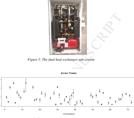
2) Energy meters installed on the dual heat exchanger units for SH and DHW inside the
188
dwelling heat interface units (HIUs) (See Figure 5) provide the supply and return hot water
189
pipes’ real-time mass flow rate and temperature, energy and volume pulse outputs, and
190
accumulated energy consumed monthly.
191
3) Building block energy meters similar to those in the HIUs at the entrance of each building
192
block were mainly used to measure the accumulated energy consumed.
193
4) District line meters measure the hot water flow rate, the H-CDHS main supply line’s supply,
194
and the boiler house’s temperature every five minutes.
195
5) The boilers sensors measure the accumulated amount of fuel consumed and the energy
196
generated by each boiler every fifteen minutes.
197
198
Figure 4: (A) Smart meter; (B) energy meter; (C) district and block meter; (D) boiler sensors
199
200
A dual pipe network transfers the heated water from the boiler house to the building
201
units, where a dual heat exchanger (“sub-system”) was installed to provide energy for space
202
heating and domestic hot water purposes.
203
As previously mentioned, a wide range of users of different socio-economic levels and
204
behavior demands are connected to the system. Since a large number of users are lower income
205
families, their energy consumption, and consequently their annual energy demand, are highly
206
dependent on their economical state and the financial support received. Thus, the management
207
office developed a prepaid energy credit system allowing each tenant to buy a credit in advance.
208
The prepaid system connects to a smart meter in each unit. Smart-meters function both as an MP
M
AN
US
CR
IP
T
AC
CE
PT
ED
and a user interface that records the costs associated with the energy consumed every half hour,
210
which tenants could use to monitor their energy usage over time.
211
212
Figure 5: The dual heat exchanger sub-system
213
214
4.1. Limitations in demand profile prediction
215
After surveying the site and reviewing the plant sizing and load prediction procedures in
216
the design stage, it was concluded that several initial simplifications were made to predict the
217
district system’s heating load. They are:
218
1) All users were treated identically, irrespective of their behaviour, socio-economical
219
background, etc., leading to a potentially significant error in load prediction. For example, while
220
some senior tenants heat their units at a higher temperature throughout the day, younger tenants
221
try lowering their heating bill as much as possible by turning off the system at night, and by
222
using it for a short time in the evening. Those for whom social welfare is the only income could
223
potentially tolerate lower interior temperatures and use less hot water than more affluent tenants.
224
These factors were not considered in detail in the early design stage.
225
2) All units were modeled following the same benchmark assumptions, while units’
226
characteristics (e.g. layout, orientation, insulation level, and window-to-wall ratio) were ignored.
227
For example, on top of developing the district heating system in 2007, the exterior facade of all
228
high-rise towers was renovated by adding a new layer over it. Also, balconies were converted to
229
solaria, primarily on the south and west sides, which could potentially compensate a large
M
AN
US
CR
IP
T
AC
CE
PT
ED
amount of heat requirements during the day due to solar gains. This highlights the potential error
231
in using standard benchmarks, which are commonly based only on floor area and building age.
232
3) System heat loss was estimated based on the operating temperature of the distribution
233
network supply (85°C) and return (70°C), and the constant heat loss per degree temperature
234
throughout the building envelope. This assumption could hold for newly renovated buildings, but
235
not for partially renovated terrace buildings (the community’s oldest buildings). In this case, the
236
oversimplified assumption underestimates heat loss and thus overestimates the demand profile
237
prediction. However, underestimating the buildings’ heat loss could partly compensate for
238
overestimating heating demands. But since the number of units in terrace buildings is less than
239
20% of the total units connected to the district system, this underestimation is not enough to
240
compensate for an exaggerated heating load prediction for high-rise units.
241
Simplifications and conservative standard methods can greatly overestimate the overall
242
energy and peak demands; cause oversized, inefficient systems with correspondingly increased
243
capital costs provoked by short cycling and increasing inefficient combustion maintenance
244
requirements; and potentially shorter lifetimes and replacement periods. Therefore, an alternative
245
method that addresses these weaknesses was evaluated.
246
4.2. Data Validation
247
To ensure accuracy, all measured data were cross validated at three different levels: unit
248
level, building level and district level. The methodology was applied to Arran tower (Tower #1)
249
and Arian tower (Tower #2).
250
In the preliminarily validation of the data collected by smart metres in the Arran Tower
251
units over four months of heating (November 2016 to February 2017), tenant occupancy was
M
AN
US
CR
IP
T
AC
CE
PT
ED
verified and any changes in unit occupancy eliminated from results to avoid errors in the unit
253
energy demand profile. After eliminating units with different tenants2, the monthly energy
254
demand of remaining units was calculated using the data collected from smart meters. The
255
monthly energy demand in units with similar tenants is expected to correlate with the monthly
256
outdoor temperature. Therefore, a unit’s monthly usage in months with similar average outdoor
257
temperatures should remain almost constant.
258
To ensure building data accuracy, the cumulated monthly usage of all units in each
259
building and the building’s linearized heat loss were calculated and compared with the building
260
meter. A similar procedure was chosen at the network level. The boiler house’s total output was
261
compared with the total accumulated energy demand of all buildings and network losses added.
262
5. Results and Conclusion
263
5.1. Primary analysis of the H-CDHS energy performance
264
In the first step, the CDHS’ two-year long monitored data was analyzed. Results showed
265
that CDHS’ existing condition operates less efficiently with a higher heat loss than the expected
266
design efficiency. Moreover, the predicted heating demand load for sizing the boiler house was
267
2-2.5 higher than the district’s actual power demand load. This over estimating caused an
268
oversizing of the boiler house. Given this, the boiler never worked at its optimal capacity and
269
most of the time operated at a partial capacity, which decreased the system’s efficiency.
270
Tenants’ behaviour is widely variable and possibly affected by individual characteristics,
271
including economic status. The preliminary analysis of the data obtained from smart meters in
272
each unit showed that units with almost identical physical characteristic have significantly
273
2
M
AN
US
CR
IP
T
AC
CE
PT
ED
different monthly energy demands. A field investigation and a recorded data reading revealed
274
that only few units used a thermostat with a given set-point value to control the space heating.
275
The majority did not use the heating system for most of a day. In most units, the heating system
276
was off day and night, or only used briefly during the day. For tenants who turned on the heating
277
more frequently, such unexpected behaviors were oversimplified in the CDHS’ design stage,
278
assuming that all tenants use thermostats to control space heating on a regular pattern day and
279
night.
280
5.2. Clustering units
281
The first step in predicting the heating load, using the four-step procedure mentioned in
282
the methodology section, is to define the number of clusters required. To do that, all the units
283
were initially divided, based on their built form and construction type, into two archetypes—the
284
newly renovated high-rise, and partially renovated old terrace buildings. The units within each
285
archetype were further segmented based on their occupancy behavior. A sample population
286
dataset was selected to define the optimal number of archetypes associated with the occupants’
287
behavior in each construction type The total energy demand [kWh], the number of inter-unit heat
288
exchanger on/off cycle per month, the peak monthly load [kW], the monthly heating degree day
289
(HDD), and average monthly outdoor temperature were determined as effective parameters for
290
defining the number of archetypes.
291
For large-scale communities with numerous users like WWH, using all monitored data
292
from every individual unit to determine the parameters required for defining the optimal cluster
293
number is computationally intensive. Instead of calculating the required parameters of all units,
294
the parameters of a smaller sample data that could represent the same distribution as the whole
M
AN
US
CR
IP
T
AC
CE
PT
ED
community were considered (Arran tower, 72 units). The results were extrapolated to the entire
296
data-set (Arian tower and the whole district).
297
Figure 6 shows Arran tower’s average monthly energy demand (for all dwelling units)
298
for both DHW and SH, between November 2016 and February 2017. This figure shows the range
299
of energy demand fluctuation when outdoor temperatures and monthly HDD do not vary
300
considerably. Variations between 5.17 [°C] and 5.98 [°C] for outdoor temperature and from 312
301
to 331 for monthly HDD (Figure 6) are not significant for most units. Results obtained for all
302
individual units in the Arran tower show that the monthly energy demand remains almost
303
constant, with unit-to-unit variation generally being much greater than that of a unit’s monthly
304
variation (except units 12, 37 and 39). Hence, most units’ demand profile’s monthly average is
305
expected to remain almost constant (Figure 7).
306
307
Figure 6: Monthly consumption of individual units in Tower # 1, Arran Tower
308
309
310
Figure 7: Outdoor temperature and HDD for the 2016-17 heating season (Nov 2016 - Feb 2017)
311
312
Using the five parameters, monthly consumption, number of inter-unit heat exchanger on/off
313
cycle per month, monthly peak demand, monthly HDD and monthly outdoor average
314
temperature, the K-means (number of clusters) varied between 1 and 20 to construct different
315
numbers of clusters. Using an R software for each value of k, the square metric distance (m²) of
316
residual (R) from a reference point was determined in order to find the optimal number of
317
archetypes (clusters) for simulation. This value was selected when the difference between the
318
residual of two consecutive clusters became negligible. One should choose a number of clusters
M
AN
US
CR
IP
T
AC
CE
PT
ED
so that adding another cluster does not significantly increase the dataset presentation. The results
320
are plotted in Figure 8, and it can be concluded that four to seven archetypes can be chosen as the
321
optimal number. Here, k-means 4 was selected as the optimal number for demonstrating the
322
method with adequate accuracy while maintaining computational costs low.
323
Given the hierarchical clustering approach, all units in the sample dataset (Tower # 1)
324
were divided into four different archetypes: Typical High Usage (NTHU) cluster 1,
Non-325
Typical Low Usage (NTLU) cluster 2, Typical Thermostat Control Usage (TTCU) cluster 3, and
326
Non-Typical Medium Usage (NTMU) cluster 4 (See Figure 9). The percentage ratio of units
327
within each archetype is shown in Figure 9.
328
329
Figure 8: Optimal number of archetypes
330
331
Results obtained from the clustering in Tower # 1 show that only 5% of units are of the
332
TTCU archetype. This value was assumed to be 100% in the CDHS’ design stage. The
333
percentage of users in other archetypes are 16% (NTLU), 24% (NTMU), and 53% (NTHU).
334
335
Figure 9: Clustering results for Tower # 1
336
337
Figure 10 shows the typical daily demand profile of the reference buildings associated
338
with each defined archetype obtained from the monitored data. It is important to note that in the
339
training stage (step 3), the annual reference building’s demand profile was used, while here only
340
a typical daily demand was presented. The heating demand profile for different occupancy
341
archetypes is similar to one reported by tenants in the field investigation. NTLU users’ profile is
342
largely dominated by a DHW usage in the morning and evening, and a slight use of space
M
AN
US
CR
IP
T
AC
CE
PT
ED
heating in the evening. NTMU users heat their space more frequently during the day, while
344
NTHU and TTCU users generally use their thermostat to control space heating for defined
345
periods. As a result, their heating profile is more continuous. NTHU users turn off their heating
346
at night, while TTCU users keep it on the whole day, with variable night and day set points.
347
348
Figure 10: Demand Profile for Reference Buildings of Each Class
349
NTLU (1), NTMU (2), NTHU (3), TTCU (4)
350
351
5.3. Predictive models
352
After training the model using data from the reference buildings, and defining the input file for
353
the remaining units, the heating demand profile of the district was predicted. The MNLR model
354
was used here to predict WWH district’s heating demand profile, trained by adopting the
non-355
linear autoregressive model with an external Input (NARX). To account for the building’s
356
thermal mass effect on the unit’s energy demand, the model used past target data, a demand
357
profile, and other series of input parameters defined earlier in this paper. To predict the demand
358
profile in future hours, previously predicted values and input files were used at the same time.
359
To determine the number of past hours required in the training stage, the model was trained with
360
different past hours ranging from 2 to 8 hours. The best fit was set as the number of past hours
361
required for representing the thermal mass of the units. For this study, 4 hours was the best fit.
362
Also in this study, the data for real H-CDHS was used to train and validate the MLNR model
363
using the above-mentioned four-step procedure. To verify the models’ flexibility to include
364
different users’ behavior, WWH’s diverse community with a wider range of users’ behavior was
365
used.
M
AN
US
CR
IP
T
AC
CE
PT
ED
Due to limitations in acquired data, the adapted methodology (Figure 5 and section 5) and
367
associated Matlab code were slightly modified [25] to further improve the model’s accuracy, as
368
explained below:
369
In addition to the reference buildings’ demand profile and three sets of input files (i.e. solar
370
dependent, internal gain dependent, and temperature dependent data files), a time-dependent
371
factor related to the DHW was also considered.
372
In the initial model [25], the indoor-outdoor temperature difference was used to generate the
373
temperature dependent data file. In this study, only the outdoor temperature was considered
374
since the units’ indoor temperature was not monitored.
375
Since the internal heat generation was not monitored in each unit, the electrical energy
376
consumed by the reference building was used to indicate the unit’s internal energy
377
generation. The existing internal generation from the British Housing Model (BHM) was
378
thus adopted and scaled down to match the energy consumption.
379
The adjusted typical thermostat control profile with a thermostat set-point of 19°C was used
380
for the common area. For the towers, the common area accounts for about 15.8% of the total
381
area of which only 45% is assumed to be conditioned.
382
Using the latter modifications, the input file for all units was generated. Moreover, the
383
reference buildings and their demand profiles were defined earlier in the clustering step. Having
384
the reference building’s input file and demand profile, the MNLR model was trained and the
385
related coefficients were determined. To verify the model’s accuracy, its prediction was
386
compared with measured data at three different levels. At the first level, the Arran tower’s
M
AN
US
CR
IP
T
AC
CE
PT
ED
(Tower #1) heating demand profile3 was predicted. At the second level, the model was applied to
388
the Arian Tower (Tower #2) and its prediction was compared with the measured data. The entire
389
district’ total energy demand was then predicted and compared with the data acquired from the
390
district’s total energy demand.
391
Energy demand prediction for the Arran tower (Tower #1)
392
In first step, the energy demand profile of the Arran tower’s (Tower #1) has been
393
predicted. The predicted profile then compared with the one obtained from measured data.
394
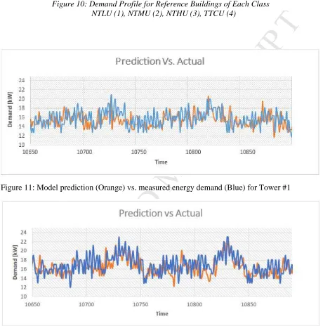
Figure 11 shows the energy demand profile for the first ten days of November 2016, where
395
appears a generally good agreement between the model’s prediction and the measured data. The
396
MSRE calculated for the data predicted was around 12.6%. A discrepancy between the two
397
curves is expected and can be attributed largely to the inevitable lack of information about
398
occupants’ inherently stochastic behaviour.
399
400
Figure 11: Model prediction (Orange) vs. measured energy demand (Blue) for Tower #1
401
402
Energy demand prediction for the Arian tower (Tower #2)
403
At the second level of model validation, the model’s prediction is validated with the
404
measured data for the Arian tower (Tower #2). No data collected from this tower was previously
405
used to generate the model associated with the units’ energy demand profile. The Arian tower
406
holds 72 units and is approximately 300 meters away from the boiler house. Figure 12 compares
407
the model’s prediction and the measured data for the first 10 days of the November 2016. A good
408
agreement can be observed. The MSRE calculated for the predicted data is around 11.2% for the
409
3
M
AN
US
CR
IP
T
AC
CE
PT
ED
whole year and 8.2% for the heating season. The predicted demand’s general trend matches the
410
measured demand. Considering the data used to generate the demand profile model was based on
411
that of occupants in a different tower, the result is remarkably good.
412
Figure 12: Model prediction (Orange) vs. measured energy demand (Blue) for Tower # 2
413
414
District energy demand prediction
415
The WWH district consists of six 12-story towers and five 4-story terrace buildings
416
connected to the boiler house through an underground piping distribution network. To predict the
417
entire WWH district system’ total energy demand, predicting the lost and delivered energies is
418
required and calculated in this section. To predict the entire WWH H-CDHS’ demand, the
419
demand of each block has to be calculated. The losses associated with the distribution system
420
itself must then be factored in.
421
The underground piping network has been used in in this project is an insulated dual pipe
422
network transferring hot water at a flow temperature of 85 ℃ and a return temperature of 70 ℃
423
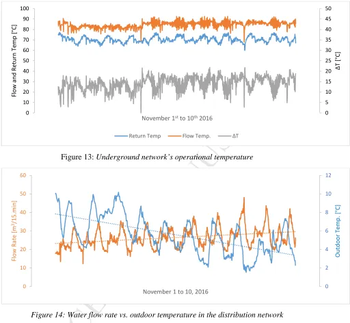
with a total length of 2.4 km (1.2 km supply and 1.2 km return). Figure 13 shows the
424
underground piping network’ operational temperature.
425
426
Figure 13: Underground network’s operational temperature
427
428
Instead of changing the room operational temperature, the underground network’s
429
operational temperature remains relatively constant during the year to control the amount of heat
430
transfer from the boiler house to the consumers. This causes the system’s mass flow rate to
M
AN
US
CR
IP
T
AC
CE
PT
ED
continuously vary during a day. Figure 14 shows the fluctuating water flow rate in the first 10
432
days of November 2016.
433
434
Figure 14: Water flow rate vs. outdoor temperature in the distribution network
435
436
Having the underground network’s total length alongside its operational temperature, the
437
supply and return pipes’ water mass flow rate, the outdoor temperature, the thermal properties of
438
the soil and pipe insulations, and the distribution network’s total heat loss can be determined. To
439
simplify the prediction process, a linear relation for the temperature difference between the
440
operational temperature and surrounding environment temperatures is pre-assumed. Figure 15
441
shows the underground distribution network’s predicted heat loss for the entire system.
442
443
Figure 15: Distribution network’s monthly heat loss projection
444
445
Since for many units the demand profiles are not available (see section 4), the energy demand
446
predicted for the entire system is compared with the total energy generated by the boiler house.
447
As stated earlier, the boiler house’s sensor measures only the accumulated amount of fuel
448
consumed and the energy generated by each boiler every fifteen minutes. Figure 16 and Table 2
449
show the district’s predicted accumulated energy demand against the energy generated by the
450
boiler house.
451
452
Figure 16: Accumulated predicted energy delivered vs actual generated energy in the boiler
453
house
454
M
AN
US
CR
IP
T
AC
CE
PT
ED
Table 2: Accumulated predicted energy delivered vs actual generated energy in the boiler
456
house and error
457 458
Results show a higher agreement between the predicted and actual energy demand with a
459
monthly discrepancy between -4% to 6%, except in January 2017, when the error was
460
approximately 30%. This error is due to a relatively high heat loss in the distribution network. In
461
January 2017, given two faulty bypass valves in two different towers, the system’s mass flow
462
rate increased. Percent and results in increasing the higher heat loss of the system compared with
463
normal condition. Over a year, the accumulated energy demand predicted (3,288,340 kWh)
464
shows a discrepancy of about 5% compared with the actual energy generated by the boiler house
465
(3,138,431 kWh). The underestimation of the total energy demand of the district is mainly due to
466
the buildings’ heat loss, especially the older 4-stories terrace building with higher envelope
467
deterioration. However, in the training process (Step 3), the reference profile obtained from the
468
Arran tower, which is better renovated comparing with the terrace buildings, was used with a
469
relatively lower heat loss. It is important to note that in the training stage, the MNLR model was
470
trained once using the reference building obtained from the Arran tower. These trained models
471
were later used to predict the heating demand profile of remaining units, only by adopting their
472
input file. Moreover, the ratio of the occupants’ behavior considered in TTCU in terrace
473
buildings was slightly higher.
474
6. Conclusion
475
The existing simplified models used for predicting the CDHSs demand lack the flexibility
476
to predict loads for diverse user types. To predict the heating demand, this study used a mid-size
477
community district energy system with diverse user types was investigated using a newly
478
proposed procedure. The main conclusion of this study can be summarized as follows:
M
AN
US
CR
IP
T
AC
CE
PT
ED
At an early design stage, the community’s heating demand profile was predicted following a
480
simplified model with an average national energy benchmark for Scotland. The only
481
adjustment made to the benchmark was a 20% reduction in the overall energy consumption
482
and peak demand to compensate for the occupants’ economic status. The results of this
483
oversimplification was overestimating the peak energy demand by a factor of 2.
484
The prediction shows high correlations between the predicted and actual profile even though
485
the heating demand profile consist of both SH and DHW usage. The suggested procedure
486
captured the profile with an acceptable accuracy level—11.2% in the annual RMSE, and
487
8.2% in the seasonal RMSE.
488
Results shows that the prediction accuracy remains close both at the building and community
489
levels due to the models’ flexibility in capturing the demand profile of every individual unit.
490
Unlike most existing models, the suggested procedure, which extrapolates the data based on
491
the number of the users or total floor area, this model predicts the community load by
492
envisaging that of every single user.
493
Acknowledgement
494
The authors would like to express their gratitude to Concordia University for the support through the 495
Concordia Research Chair – Energy & Environment. 496
497
References
498
1. Implementation of the Energy and Climate Package, P.H.A.F.S. COMMITTEE
499
ON ENVIRONMENT, Editor. 19 April 2011, European Parliament - national
500
Parliaments.
501
2. Pathways to a Clean Energy System, I.E. Agancy, Editor. 2012, Energy
502
Technology Perspectives 2012.
503
3. Bastani, A. and F. Haghighat, Expanding Heisler chart to characterize heat
504
transfer phenomena in a building envelope integrated with phase change
505
materials. Energy and Buildings, 2015. 106: p. 164-174.
M
AN
US
CR
IP
T
AC
CE
PT
ED
4. Mastani Joybari, M., F. Haghighat, and S. Seddegh, Numerical investigation of a
507
triplex tube heat exchanger with phase change material: Simultaneous charging
508
and discharging. Energy and Buildings, 2017. 139: p. 426-438.
509
5. Nkwetta, D.N., et al., Phase change materials in hot water tank for shifting peak
510
power demand. Solar Energy, 2014. 107: p. 628-635.
511
6. Thieblemont, H., F. Haghighat, and A. Moreau, Thermal Energy Storage for
512
Building Load Management: Application to Electrically Heated Floor. Applied
513
Sciences, 2016. 6(7): p. 194.
514
7. Canada’s Energy Future 2013 - Energy Supply and Demand Projections to 2035.
515
Available from:
https://www.neb-one.gc.ca/nrg/ntgrtd/ftr/2013/ppndcs/ppndcs-516
eng.html.
517
8. Talebi, B., et al., A Review of District Heating Systems: Modeling and
518
Optimization. Frontiers in Built Environment, 2016. 2(22).
519
9. Zhao, H.-x. and F. Magoulès, A review on the prediction of building energy
520
consumption. Renewable and Sustainable Energy Reviews, 2012. 16(6): p.
521
3586-3592.
522
10. Olsthoorn, D., F. Haghighat, and P.A. Mirzaei, Integration of storage and
523
renewable energy into district heating systems: A review of modelling and
524
optimization. Solar Energy, 2016. 136: p. 49-64.
525
11. Heiple, S. and D.J. Sailor, Using building energy simulation and geospatial
526
modeling techniques to determine high resolution building sector energy
527
consumption profiles. Energy and Buildings, 2008. 40(8): p. 1426-1436.
528
12. Theodoridou, I., A.M. Papadopoulos, and M. Hegger, A typological classification
529
of the Greek residential building stock. Energy and Buildings, 2011. 43(10): p.
530
2779-2787.
531
13. Powell, K.M., et al., Heating, cooling, and electrical load forecasting for a
large-532
scale district energy system. Energy, 2014. 74: p. 877-885.
533
14. Nielsen, H.A. and H. Madsen, Modelling the heat consumption in district heating
534
systems using a grey-box approach. Energy and Buildings, 2006. 38(1): p. 63-71.
535
15. Lee, Y.-S. and L.-I. Tong, Forecasting energy consumption using a grey model
536
improved by incorporating genetic programming. Energy Conversion and
537
Management, 2011. 52(1): p. 147-152.
538
16. Filogamo, L., et al., On the classification of large residential buildings stocks by
539
sample typologies for energy planning purposes. Applied Energy, 2014. 135: p.
540
825-835.
541
17. S.Narmasara, F.G.H.K.L.G.B., SIMPLIFIED BUILDING MODEL OF DISTRICTS
542
in Fifth German-Austrian IBPSA Conference 2014: RWTH Aachen University. p.
543
152-159.
544
18. Eicker:, U., POLYCITY – Europäische Energieforschung für Kommunen.,
545
S.B.S.d. Sonnenenergie, Editor. Oktober 2004. .
546
19. Tuominen, P., et al., Calculation method and tool for assessing energy
547
consumption in the building stock. Building and Environment, 2014. 75: p.
153-548
160.
549
20. Galante, A. and M. Torri, A methodology for the energy performance
550
classification of residential building stock on an urban scale. Energy and
551
buildings, 2012. 48: p. 211-219.
M
AN
US
CR
IP
T
AC
CE
PT
ED
21. Mavrogianni, A., et al. A GIS-based bottom-up space heating demand model of
553
the London domestic stock. in Proceddings 11th International IBPSA
554
Conference, Building Simulation. 2009.
555
22. Pedersen, L., J. Stang, and R. Ulseth, Load prediction method for heat and
556
electricity demand in buildings for the purpose of planning for mixed energy
557
distribution systems. Energy and Buildings, 2008. 40(7): p. 1124-1134.
558
23. Dotzauer, E., Simple model for prediction of loads in district-heating systems.
559
Applied Energy, 2002. 73(3–4): p. 277-284.
560
24. Mavrogianni, A., et al., Space heating demand and heatwave vulnerability:
561
London domestic stock. Building Research & Information, 2009. 37(5-6): p.
583-562
597.
563
25. Talebi, B., F. Haghighat, and P.A. Mirzaei, Simplified model to predict the thermal
564
demand profile of districts. Energy and Buildings, 2017. 145: p. 213-225.
565
26. Fonseca, J.A. and A. Schlueter, Integrated model for characterization of
566
spatiotemporal building energy consumption patterns in neighborhoods and city
567
districts. Applied Energy, 2015. 142: p. 247-265.
568
27. Gadd, H. and S. Werner, Daily heat load variations in Swedish district heating
569
systems. Applied Energy, 2013. 106: p. 47-55.
570
28. Caputo, P., G. Costa, and S. Ferrari, A supporting method for defining energy
571
strategies in the building sector at urban scale. Energy Policy, 2013. 55: p.
261-572
270.
573
29. Nouvel, R., et al., CityGML-based 3D city model for energy diagnostics and
574
urban energy policy support. IBPSA World, 2013. 2013: p. 1-7.
575
30. Ali, M.T., et al., A cooling change-point model of community-aggregate electrical
576
load. Energy and Buildings, 2011. 43(1): p. 28-37.
577
31. Goia, A., C. May, and G. Fusai, Functional clustering and linear regression for
578
peak load forecasting. International Journal of Forecasting, 2010. 26(4): p.
700-579
711.
580
32. Tanimoto, J., A. Hagishima, and H. Sagara, A methodology for peak energy
581
requirement considering actual variation of occupants’ behavior schedules.
582
Building and Environment, 2008. 43(4): p. 610-619.
583
33. Shimoda, Y., et al., Residential end-use energy simulation at city scale. Building
584
and Environment, 2004. 39(8): p. 959-967.
585
34. Lund, H., et al., 4th Generation District Heating (4GDH). Energy, 2014. 68: p.
1-586
11.
587
M
AN
US
CR
IP
T
AC
CE
[image:26.595.38.548.131.662.2]PT
ED
Table 1: Load Prediction Summary
Author Ref Year Prediction
period Prediction Type/Resolution Method
Fonsenca et al. [26] 2015 Annual Total Energy Demand Simplified Modeling/ Adjusted HDD
Powell et al. [13] 2014 Daily One day forecasting NARX**; ANN
Tuominen et al. [19] 2014 Annual Total Energy Demand Linear Development Using REMA Filogamo et al. [16] 2014 Annual Total Energy Demand Simplified Equivalent RC
Koene et al. [17] 2014 Annual Total Energy Demand Simplified Equivalent RC
Gadd et al. [27] 2013 Daily Average Daily and Hourly
Variation Time Series
Caputo et al. [28] 2013 Annual Total Energy Demand Comprehensive Modeling Nouvel et al. [29] 2013 Annual Total Energy Demand Quasi State Monthly Energy Balance Galante et al. [20] 2012 Annual Total Energy Consumption Linear Regression Analysis
Ali et al. [30] 2011 Annual Peak Load and Total Demand Multivariant Regression Lee et al. [15] 2011 Annual Total Energy Demand Gray Box Model Theodoridou et
al. [12] 2011 Annual Annual Peak Demand Comprehensive Modeling
Goia et al. [31] 2010 Monthly Peak Load Forecasting Linear Regression & Clustering Mavrogianni [21, 24] 2009 Annual Annual Heating Degree Day Linear Regression Linda Pedersen
et al. [22] 2008 Annual Linearized peak Day Profile* Linear Regression
Ihara et al. 2008 Annual Total Energy Demand Gray Box
Heiple et al. [11] 2008 Annual Hourly / Total Energy Demand Software Modeling, "eQUEST"
Nielsen et al. [14] 2006 Annual Profile Gray Box
Tanimoto et al. [32] 2008 Annual Peak Demand Stochastic method
Koroneos 2005 Annual Total Energy Demand Gray Box
Ratti et al. 2004 Annual Total Energy Demand Multivariant Regression
Shimoda et al. [33] 2004 Annual Total EUI / Total Energy
Demand Software Modeling, "SCHEDULE" Eicker [18] 2004 Annual Total Energy Demand Simplified Equivalent RC
M
AN
US
CR
IP
T
AC
CE
PT
ED
Predicted Actual
Error Monthly Accumulated Monthly Accumulated
Apr-16 265000 265000 282000 282000 6%
May-16 301003 566003 293610 575610 -3%
Jun-16 424837 990840 409140 984750 -4%
Jul-16 175360 1166200 168770 1153520 -4%
Aug-16 189030 1355230 185340 1338860 -2%
Sep-16 173552 1528782 177190 1516050 2%
Oct-16 259411 1788193 266710 1782760 3%
Nov-16 356885 2145078 368310 2151070 3%
Dec-16 388553 2533631 429580 2580650 10%
Jan-17 245779 2779410 349300 2929950 30%
Feb-17 359021 3138431 358390 3288340 0%
M
AN
US
CR
IP
T
AC
CE
PT
ED
M
AN
US
CR
IP
T
AC
CE
PT
ED
Figure 2: Hybrid community-district heating system layout in Whitlawburn, Cambuslang, Scotland
Tower Terrace
M
AN
US
CR
IP
T
AC
CE
PT
ED
M
AN
US
CR
IP
T
AC
CE
PT
ED
[image:31.595.100.535.137.519.2]Figure 4: (A) Smart meter; (B) energy meter; (C) district and block meter; (D) boiler sensors
Figure 5: The dual heat exchanger sub-system
M
AN
US
CR
IP
T
AC
CE
PT
ED
Figure 7: Outdoor temperature and HDD for the 2016-17 heating season (Nov 2016 - Feb 2017)
M
AN
US
CR
IP
T
AC
CE
PT
ED
Figure 9: Clustering results for Tower # 1
0 1 2 3 4
0 5 10 15 20
C
o
n
su
m
p
ti
o
n
[
k
W
h
]
Time of Day
M
AN
US
CR
IP
T
AC
CE
PT
ED
0 1 2 3 40 5 10 15 20
C o n su m p ti o n [ k W h ]
Time of Day
Typical Daily NTMU Profile During Heating Period
0 1 2 3 4
0 5 10 15 20
C o n su m p ti o n [ kW h ]
Time of Day
Typical Daily NTHU Profile During Heating Period
0 1 2 3 4
0 5 10 15 20
C o n su m p ti o n [ k W h ]
Time of Day
M
AN
US
CR
IP
T
AC
CE
[image:35.595.69.529.163.627.2]PT
ED
Figure 10: Demand Profile for Reference Buildings of Each Class NTLU (1), NTMU (2), NTHU (3), TTCU (4)
Figure 11: Model prediction (Orange) vs. measured energy demand (Blue) for Tower #1
M
AN
US
CR
IP
T
AC
CE
PT
ED
Figure 13: Underground network’s operational temperature
Figure 14: Water flow rate vs. outdoor temperature in the distribution network
0 5 10 15 20 25 30 35 40 45 50 0 10 20 30 40 50 60 70 80 90 100 ∆ T [ °C ]
November 1stto 10th2016
F lo w a n d R e tu rn T e m p [ °C ]
Return Temp Flow Temp. ∆T
0 2 4 6 8 10 12 0 10 20 30 40 50 60 O u td o o r T e m p . [° C ]
November 1 to 10, 2016
[image:36.595.68.580.104.576.2]M
AN
US
CR
IP
T
AC
CE
PT
ED
[image:37.595.67.542.105.535.2]Figure 15: Distribution network’s monthly heat loss projection
Figure 16: Accumulated predicted energy delivered vs actual generated energy in the boiler house
0 10 20 30 40 50 60
H
e
a
t
Lo
ss
[
M
W
h
]
Monthly Heat Loss August 2016 - May 2017
5,00,000 10,00,000 15,00,000 20,00,000 25,00,000 30,00,000 35,00,000
Jan-16 Mar-16 May-16 Jun-16 Aug-16 Oct-16 Nov-16 Jan-17 Mar-17
Actual
M
AN
US
CR
IP
T
AC
CE
PT
ED
Highlights
Simplified method is used to predict the heating load of a mid-size community.
Clustering approach is used to define the number of archetypes required for the load prediction.