City, University of London Institutional Repository
Citation
:
Xu, G., Yan, S. & Ma, Q. (2015). Modified SFDI for fully nonlinear wavesimulation. CMES - Computer Modeling in Engineering and Sciences, 106(1), pp. 1-35. doi: 10.3970/cmes.2015.106.001
This is the accepted version of the paper.
This version of the publication may differ from the final published
version.
Permanent repository link:
http://openaccess.city.ac.uk/12462/Link to published version
:
http://dx.doi.org/10.3970/cmes.2015.106.001Copyright and reuse:
City Research Online aims to make research
outputs of City, University of London available to a wider audience.
Copyright and Moral Rights remain with the author(s) and/or copyright
holders. URLs from City Research Online may be freely distributed and
linked to.
Modified SFDI for Fully Nonlinear Wave Simulation
Guochun Xu1, S Yan2, Q.W. Ma2, 1
1: College of Shipbuilding Engineering, Harbin Engineering University, Harbin, China 2: School of Mathematics, Computer Sciences and Engineering, City University London, EC1V 0HB
Abstract: In the Meshless Local Petrove-Galerkin based on Rankine source solution (MLPG-R), a simplified finite difference interpolation (SFDI) scheme was developed for numerical interpolation and gradient calculation (CMES, Vol. 23(2), pp. 75-89). Numerical tests concluded that the SFDI is generally as accurate as the linear moving least square method (MLS) but requires less CPU time. In this paper, a modified SFDI is proposed for numerically modelling of nonlinear water waves, considering the typical feature of the spatial variation of the wave-related parameters. Systematic numerical investigations are carried out and the results indicate that the modification considerably improves the robustness of the SFDI on gradient estimation. Although the scheme is originally derived for meshless method, its feasibility and accuracy in the mesh-based methods are discussed here through the fully nonlinear wave simulation using the Quasi Arbitrary Lagrangian Eulerian Finite Element Method (QALE-FEM), which is based on fully nonlinear potential theory.
Keywords: Modified SFDI, gradient estimation, nonlinear water waves, QALE-FEM
1. Introduction
Numerical interpolation and gradient estimation are essential in the meshless methods, e.g. the Meshless Local Petrove-Galerkin (MLPG) method developed by Atluri and Zhu (1998), the moving particle semi-implicit method (MPS) developed by Koshizuka and Oka (1996) and the smooth particle hydrodynamics(SPH, e.g. Zheng, Ma and Duan, 2014). They include the Shepard function, the partition of unity, the
reproducing kernel particle interpolation, the radial basis function, and the moving least square methods (MLS). Detailed reviews can be found in Atluri and Shen (2002) and Ma (2008).
Ma (2008) developed a new meshless interpolation scheme called simplified finite difference interpolation (SFDI). The numerical investigations concluded that the SFDI is generally as accurate as the linear MLS but requires less CPU time due to the fact that the SFDI requires the inverse of lower order matrix than the MLS. It is also observed that the SFDI is more robust than the schemes used in the MPS (e.g. Yoon, Koshizuka and Oka, 2001). The SFDI has been implemented in the MLPG Method Based on Rankine Source Solution (MLPG_R) developed by Ma (2005) and the SPH method to modelling breaking waves and their impacts on structures, e.g. Sriram and Ma (2012), Zhou and Ma (2010) and Zheng, Ma and Duan (2014).
solvers and the meshless methods, e.g. Sriram and Ma (2014), have therefore been developed to accelerate the simulation. In the FNPT models, the flow is governed by the Laplace Equation of the velocity potential ( ). Various methods, such as the boundary element method (BEM, e.g. Fochesato and Dias, 2006) and the finite element method (FEM), can be used to solve the FNPT model using mixed Eulerian and Lagrangian (MEL) approach as reviewed by Ma and Yan (2006), Yan and Ma (2010), who also concluded that the FEM is more robust than BEM in modelling fully nonlinear water waves. In the FNPT based FEM methods, the fluid velocity on the free surface is estimated by the gradient of and it is
essential to provide the position of and the values of at the free surface for next time
step. For this purpose, various schemes have been developed. They include the shape function, global projection Galerkin method (Wu and Eatock Taylor, 1994), least square method (Ma, Wu and Eatock, 2001), mapped finite difference scheme (Steinhagen, 2001), cubic spline method (Sriram, Sannasiraj and Sundar, 2010). Their advantage and limitation have been discussed by Sriram, Sannasiraj and Sundar (2010), in which a systematic investigation concluded that the cubic spline method was superior over other methods when modelling strong nonlinear waves but was limited to two-dimensional (2D) applications. Ma and Yan (2006) suggested a hybrid scheme to estimate tangential and normal velocity separately. To find the normal velocity component at each free-surface node, a three-point finite difference scheme was used, in which a quadratic MLS was adopted to interpolate the velocity potential at two other points in its normal direction. A linear least square method was implemented to estimate the tangential components. By using this scheme, a promising accuracy was confirmed for 2D or three dimensional (3D) nonlinear waves including overturning (Yan and Ma, 2010).
However, in the above-mentioned interpolation and gradient calculation schemes derived either for meshless or mesh based methods, it is generally assumed that the variation of a variable features the same in all directions in the physical coordinate system, e.g. an isotropous basis functions (such as [1,x,y,z]
for linear interpolation) are used in the least square or MLS methods. In fact, the variations of wave-related parameters, e.g. the velocity potential and the pressure, show significantly different features in horizontal and vertical directions. Taking the 2D linear regular wave as example, the velocity potential satisfies
kh h z k kx t ag
cosh ) ( cosh )
sin(
(1a)
for waves in finite depth and
kz
e kx t ag
) sin(
(1b)
It should be pointed out that, provided sufficiently fine particle or mesh resolution, both sinusoidal function and the exponential function can be well approximated by using polynomials. However, one may agree that the convergence property of the interpolation schemes may be improved if the different features of spatial variations are considered. In this paper, the SFDI is modified by considering the typical feature of the wave-related parameters in the vertical direction. A systematic investigation is carried out to show its improved convergence property. Another contribution of this paper is to apply the modified SFDI to the Quasi Arbitrary Lagrangian Eulerian Finite Element Method (QALE-FEM), which is based on FNPT and has been proved to be much more efficient compared to other numerical methods at the same accuracy level (Yan and Ma, 2010).
2. Modified SFDI scheme for gradient estimation
The detailed derivation of the SFDI for the gradient estimation has been given in Ma (2008). It will not be repeated here. In order to consider the feature of the spatial variation of wave-related parameters, such as the pressure in the MLPG_R (Sriram and Ma, 2012) and SPH (Zheng, Ma and Duan, 2014) or the velocity potential in the FNPT models (e.g. Yan and Ma, 2010), as discussed in the Introduction, it is proposed to estimate the
gradient in a homogeneous space (1,2,3) instead of the physical space (x,y,z), in which
h y h
x/ , 2 /
1
and two definitions of 3 listed below are considered in the investigation,
) cosh( )) ( cosh( 3 h z h
(2a)
z
e
3 (2b)
where is a coefficient. It is easy to deduce
that, if k, Eqs. (2a) and (2b) represent the
depth variation functions for linear regular wave in finite depth and deep water, respectively. For clarity, the modified SFDI with Eq. 2(a) and that with Eq. 2(b) are referred to as MSFDI_1 and MSFDI_2, respectively. It is worth noting that as
increases, ) cosh( )) ( cosh( h z h
approaches ez and
therefore MSFDI_1 and MSFDI_2 becomes consistent.
Following Ma (2008), f(r) is used to
represent any parameters in general where }
, , {1 2 3
r denoting the position vector of a
point in the homogeneous space. At any particle/node J with position vector rJ, it can
be estimated using the Taylor expansion at particle/node O with r0, such as the following
form with linear accuracy,
2
0 0
0) ( )
( ) (
0 r r O r r
f r f r
f J r J J
(3)
Multiplying 2 ,0 0 , 0 , J J J w r r r r m m
where wJ,0 is
the weight function for particle/node J related to r0
, on both sides of Eq. (3), taking the sum
of equations at all relevant particles/nodes and ignoring error term, it follows that
NJ k k m r
J J J J N J r J J J N J J J J J k k k m m m m m m m f w r r r r r r f w r r r r w r r r r r f r f 1 3 , 1 , 0 , 2 0 , 0 , , 0 , 1 , 0 , 2 0 2 , 0 , 1 0 , 2 0 , 0 , 0 0 0 ) ( ) ( (4)
where k and m ranging from 1 to 3;
k
J
r ,
is the
k
-directional component of the position vector
J
r ,
0 ,k r
f is the k-directional gradient of the
unknown function at position r0. Eq. (4) can
} ]{ [ } ]{
[A F C F (5)
in which
T r rr f f
f
F} [ , , ]
{ 0 3 0 2 0
1 , ,
,
,
TN
J f r f r f r
r f r f r f r f r f F ] ,..., ,..., , [ } { 0 0 0 2 0 1
[C] is an 3×N matrix with its components defined as 0 , 2 0 , 0 , , 0 1 J J J xm mJ w r r r r n
C m m
and
N J J J J xm w r r r rn m m
1 0 , 2 0 2 , 0 , ,
0
[A] is an 3×3 matrix with its entries given by
N J J J J J xm mk w r r r r r r nA m m k k
1 0 , 2 0 , 0 , , 0 , , 0 1
when mk and Amk 1 otherwise.
Through solving Eq. (5), the gradient,
0 1 , r
f ,
0 2
, r
f and
0 3
, r
f can be found and the
gradient in the physical coordinate system
(x,y,z) ,
0 ,x r
f ,
0 ,y r
f and
0 ,z r
f can be
estimated using
x f r 1 , 0 1 ,
y f r 2 , 0 2 and
z f r 3 , 0 3 , respectively. It shall be noted that
for 2D cases where x and z are considered, the following solution can be directly obtained,
h A A C A C fx r31 13 03 13 01 , 1 0
(6a)
z A A C A Cfz r
3 31 13 03 31 03 , 1 0 (6b)
Similar to the original SFDI for gradient estimation in Ma(2008), Eqs. (5) and (6) gives exact value of gradient components, independent of the distribution of particles/nodes, if f(r) is linear. If k, for 2D linear water waves, the velocity potential in the homogeneous space defined above can be written as
3 1)
sin(
ag tkh (7)
For specific horizontal location, the velocity
potential is linear in 3 and thus Eq. (6b) leads to exact solution of the vertical gradient. However, in the physical coordinate system (x,z), is not linear neither in horizontal nor
in vertical direction. Clearly the modified SFDI leads to more accurate results than the original SFDI. However, it should be noted that for nonlinear water waves, the velocity potential consist of linear component as shown in Eq. (1) and nonlinear components which do not behave the same vertical variation as the linear harmonic. For example, for 2nd- order regular waves in finite depth, two additional 2nd-order terms are introduced to Eq. (1), leading to G a kh h z k kx t G a kh h z k kx t ag 2 2 2 cosh ) ( 2 cosh ) 2 2 sin( cosh ) ( cosh ) sin( (8)
Where Gand G are the coefficients for 2nd order sub-harmonic and super-harmonic, respectively (Schaffer, 1996). The latter
follows kh h z k 2 cosh ) ( 2 cosh
in the vertical direction.
More importantly, for nonlinear wave groups consists of many wave components with different wave numbers, yielding different vertical variation. This is the main reason why a coefficient , instead of wave number k, is
adopted in Eq. (2). Sensitivity investigations in terms of are therefore required to determine the coefficient for general wave problems. It should be noted that once wave breaking occurs, the wave-related parameters near the breaking jets may not behaviour as discussed above. Such cases will not be considered in this paper.
gradient of the velocity potential). In their scheme, the physical coordinate system was transferred to a mapped coordinate aiming to normalise the vertical coordinate using
) , (
3
y x h
z h
in which (x,y) was the free
surface elevation at (x,y). The intention of such transformation was to map the computational mesh into a rectangular domain, benefiting the finite difference scheme. It did not explicitly reflect the feature of the vertical variation of wave-related parameters.
3. QALE-FEM for modelling nonlinear water waves
Although the MSFDI developed in this paper can be applied to both the meshless methods, e.g. the MLPG_R, and the mesh based methods, its overall effectiveness on modelling nonlinear water waves is demonstrated by its application to the FEM. The details of the QALE-FEM can be found in Ma & Yan (2006) and Yan & Ma (2010). A summary is given below for completeness.
In the QALE-FEM method, the flow is governed by the Laplace equation of the velocity potential. At every time step, a boundary value problem for the velocity potential is solved using the FEM. Velocities at the free surface are evaluated and used to update the free surface condition at the next time step. It should be noted that in this time-marching process, the error of the velocity estimations on the free surface in the current time step will be brought to the next time step and, therefore, may be accumulated during the time-domain simulation. Due to this fact, the velocity estimation in the FNPT modelling is required to have sufficiently high accuracy in order to achieve a satisfactory overall accuracy. As indicated above, in the previous applications of the QALE-FEM, a robust hybrid scheme is used to find the velocity in which a three-point
finite difference scheme and a linear least square method are implemented to evaluate the normal and tangential velocity components, respectively. This method is referred to as ‘3-point’ scheme in this paper.
The QALE-FEM simulation is carried out in time domain. The mesh is generated only once in the beginning of the simulation and moves to conform to the deformation of the free surface. The initial mesh used is unstructured and generated by using the in-house mesh generator. To reflect the complexity of the fluid domain, one may assign different representative mesh size (ds) to the mesh generator, which indicates the characteristic distance between two connected nodes. Although this mesh size is not precisely equal to the real mesh size, it largely indicates how fine the mesh is. It should be noted that the initial mesh can be generated using any mesh generator with any degrees of complexity, either structured or unstructured, or even mixed. Based on previous convergence investigations on modelling nonlinear water waves, for free surface elements ds is assigned to be λ/30~λ/60 depending on the wave steepness, where λ is the incident wavelength. ds gradually increases in vertical direction from the free surface to the seabed following exponential principle suggested by Wu and Eatock Taylor (1994, 1995) , i.e.
e e h x z
z
N i
i
1 1 ) (
/
(9)
in which Nz is the number of nodes in vertical
direction, Ψ the exponential coefficient which is taken as 1.7 in the investigation. Convergent test indicates that Ψ =1.7 and Nz ranging from
14 to 20 are suitable for solitary waves and nonlinear waves with frequencies ranging from
0.5~6 h/g, coving most of the application in
4. Convergent rate of MSFDI
In this section, investigations will be made into the convergent rate of the modified SFDI in gradient estimation. Well-established wave theories including the Stokes 5th order theory for regular waves (Fenton, 1985) and 2nd order wave theory for wave groups (Schaffer, 1996; Toffoli, Onotato, Babanin, Bitner-Gregersen, Osborne and Monbaliu, 2007), are used to provide analytical solutions to the wave elevation ( ), velocity potential ( ) and
velocity, for comparison. In the investigation, the velocity potential at every particle/node is specified using the wave theories. The velocity, i.e. the gradient of the velocity potential, is estimated using different gradient estimation schemes and compared with the analytical solution from the wave theories. The error is defined by
N
J a N
J
a n
v v v
1 2 1
2
(10)
where vn and va are the numerical estimations
and the analytical solutions of the velocity vector by the wave theories, respectively. It represents the relative error in terms of kinetic energy of the water waves covering the spatial domain. Although these schemes can be used for 3D non-breaking water wave problems, the numerical tests will be focused on 2D, which providing a good insight of their effectiveness and the robustness.
The spatial domain in the test is bounded by two vertical lines, the free surface (z = (x))
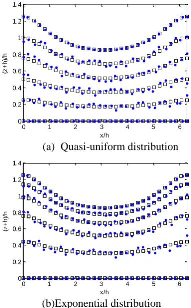
and a flat seabed (z = –h). In the horizontal direction, the particles initially distribute with a uniform distance dx as illustrated by the hollow squares in Fig. 1. Two sets of vertical distributions are considered. In the first set, a
uniform vertical distance
) / int(
) (
dx h
h x
is used.
Considering the fact that (x) changes at
different location, therefore the vertical particle distance dzis not constant but a function of x. This refers to as the quasi-uniform distribution in this paper. In the second set, the particles distributes in the vertical direction following Eq. (9). This refers to as the exponential distribution. The quasi-uniform distribution is generally used in the meshless method and the exponential distribution is commonly seen in the FNPT based FEM solvers, including the QALE-FEM, as discussed above. In order to reflect the movement of the particles/nodes during the simulation, random shifts, similar to Ma (2008), are introduced for particles as illustrated by solid diamond in Fig.1. Such random shifts are used in all cases presented in this paper.
(a) Quasi-uniform distribution
(b)Exponential distribution
Figure 1: Example of distributions of particles (Hollow: initial distribution; Solid: with random shift)
There are many options for the weight functions. In this paper, we mainly concern about effectiveness of the modification, only
0 1 2 3 4 5 6
0 0.2 0.4 0.6 0.8 1 1.2 1.4
x/h
(z
+
h
)/
h
0 1 2 3 4 5 6
0 0.2 0.4 0.6 0.8 1 1.2 1.4
x/h
(z
+
h
)/
[image:7.595.316.507.355.663.2]the following weight function is employed in all the cases,
1 0
1 5 . 0 3 / 4 4 4 3 / 4
5 . 0 4
4 3 / 2
3 2
3 2
0 ,
s s s
s s
s s
s wJ
(11) where sdJ0/rs, dJ0 and rs are, respectively,
the distance from particle/node J to O and the radius of the support domain. This function was suggested by Atluri and Zhu (1998) and has been applied to the QALE-FEM for interpolating the velocity potential using MLS, confirming its promising efficiency (Ma and
Yan, 2006; Yan and Ma, 2010). wJ,0may be
calculated in either the physical domain or the homogeneous domain. For clarity, they are
referred to as w(x,y,z) and w(1,2,3) ,
respectively.
In meshless methods, the support domain is selected based on the distances of the surrounding particles to r0
. For example, in the
MLPG_R (Ma, 2008), the size of the support domain is given by rs h4o where is a
scale factor and h4O is the distance between r0
and the fourth nearest neighbour. It may be less effective for the exponential distribution or non-uniform distribution, when dx is significant different from dz, because the particles in the support domain of r0 may not distribute on one
or more quadrants of r0 leading to lower accuracy. Alternatively, in the mesh based method, one may take advantage of the mesh connectivity and use an approach suggested by Yan (2006). In this approach, for any node O, all nodes connected to it are defined as 1st-layer nodes and those connected to the 1st-layer but not belonging to 1st-layer or itself are defined as 2nd-layer nodes, as illustrated in Fig.2. In general, mth –layer nodes are those connected to (m-1)th-layer nodes but not belonging to all the nodes on the lower layers. Once a proper number of layers are selected, the nodes used
for the numerical interpolation of gradient estimation are determined and rs hmax ,
where and hmax are scale factor and the
maximum distance from neighbour to O, is used for the weigh function. If r0
does not lay
on any nodes, the nearest node will be considered.
Figure 2: Node O and it neighbours (hollow: first-layer nodes of node O; solid: second-layer nodes of O)
This approach ensures that the neighbour nodes distribute on all quadrants of r0 except the
boundary nodes. It is easy to deduce that in the cases with quasi-uniform node distribution, this approach leads to a similar support domain to the one suggested by Ma (2008). More importantly, this approach is independent of distance and therefore ensures that the coordinate transformation does not affect the selection of the nodes/particles for the gradient estimations. This approach will be used in the test and different layers of neighbours (Nl) will
be considered to investigate the effects of the support domain size on the accuracy or the convergent rate of the modified SFDI.
3.1 Regular waves
As discussed above, Eq. (2a) and (2b) corresponds to regular waves in finite depth and deep water, respectively. In fact, Eq. (2b) is a special case of Eq. (2a). In this section, kh will vary from 0.5 to 10π to cover both shallow water and deep water waves. Different wave steepness ka ranging from 0.01 to 0.2 are used. The length of the computational domain is taken as one wavelength λ. The 5th-order
stokes theory (Fenton ,1985) is used to provide the analytical solutions to the free surface profile and velocity potential, with which different gradient estimation schemes are used to evaluate the velocity at all particles. It also provides the analytical solutions to the velocity for the error evaluation using Eq. (10).
3.1.1 Quasi-Uniform particle distribution
Fig.3 and Fig.4 shows the convergent rates of different schemes to estimate the velocity in the case with kh =2, i.e. a typical wave in finite depth, in which a quasi-uniform distribution with random shift is employed. The number of particles in x-direction Nx = λ/dx and the
numerical of particles in z-direction Nz = h/ dx.
Two layers of neighbour particles, i.e. Nl = 2,
are used to form the support domain. kis applied.
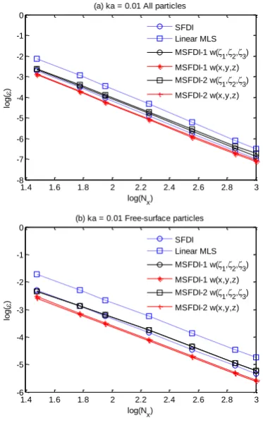
Figure 3: Convergent rate of gradient estimation for kh=2 and ka = 0.01 (quasi-uniform distribution, Nl= 2, k)
From them, it is found that the errors of all schemes decrease if more particles are distributed in the same domain. Their rates of deduction are relatively constant. The modified SFDI with weighting calculated in the physical domain, i.e. w(x,y,z) , is found to have
considerably higher accuracy at all particles than the SFDI and the linear MLS for any particle resolutions (Figs 3(a) and Fig.4(a)). The improvement is more significant when estimating the velocities at the free-surface particles (Figs. 3(b) and 4(b)). It is also interested to find that the effectiveness of the modification on improving the accuracy or the convergent rate is independent of wave steepness, although the idea of the modification origins from the linear wave theory.
Figure 4: Convergent rate of gradient estimation for kh=2 and ka = 0.2 (quasi-uniform distribution, Nl= 2, k)
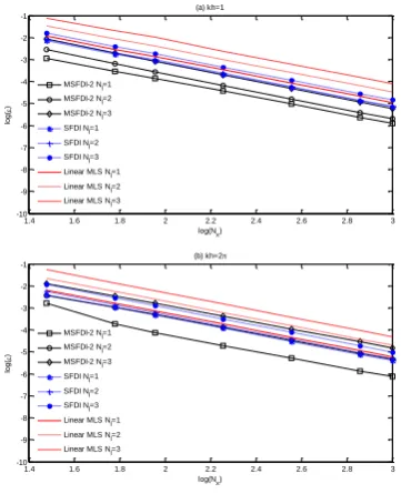
Improvement is also found in the cases with other values of kh. Some examples are given in Fig. 5 in which results from both a shallow water case with kh = 1 and a deep water case with kh =2π are displayed. For clarity, only the
1.4 1.6 1.8 2 2.2 2.4 2.6 2.8 3
-8 -7 -6 -5 -4 -3 -2 -1 0
log(Nx)
lo
g
(
)
(a) ka = 0.01 All particles
SFDI Linear MLS
MSFDI-1 w(1,2,3)
MSFDI-1 w(x,y,z)
MSFDI-2 w(1,2,3)
MSFDI-2 w(x,y,z)
1.4 1.6 1.8 2 2.2 2.4 2.6 2.8 3
-6 -5 -4 -3 -2 -1 0
log(Nx)
lo
g
(
)
(b) ka = 0.01 Free-surface particles
SFDI Linear MLS
MSFDI-1 w(1,2,3)
MSFDI-1 w(x,y,z)
MSFDI-2 w(1,2,3)
MSFDI-2 w(x,y,z)
1.4 1.6 1.8 2 2.2 2.4 2.6 2.8 3
-8 -7 -6 -5 -4 -3 -2 -1 0
log(Nx)
lo
g
(
)
(a) ka = 0.2 All particles
SFDI Linear MLS
MSFDI-1 w(1,2,3)
MSFDI-1 w(x,y,z)
MSFDI-2 w(
1,2,3)
MSFDI-2 w(x,y,z)
1.4 1.6 1.8 2 2.2 2.4 2.6 2.8 3
-6 -5 -4 -3 -2 -1 0
log(Nx)
lo
g
(
)
(b) ka = 0.2 Free-surface particles
SFDI Linear MLS
MSFDI-1 w(1,2,3)
MSFDI-1 w(x,y,z)
MSFDI-2 w(1,2,3)
[image:9.595.318.512.346.648.2] [image:9.595.81.268.394.696.2]error variation of the velocity on the free surface particles for nonlinear cases with ka = 0.2 are shown. Comparing the results shown in Figs. 3-5, one may observe that the difference between MSFDI-1 and MSFDI-2 becomes more invisible as kh increases, confirming our previous discussion on the consistence of Eq. 2(a) and (b) for deep water waves; and that the difference between the results with w(x,y,z)
and those with w(1,2,3) becomes more significant as kh increases, giving confirmation of the superiority of w(x,y,z) over
) , , (1 2 3
w in terms of accuracy of the
modified schemes.
Figure 5: Convergent rate of gradient estimation for nonlinear regular waves ka = 0.2 (quasi-uniform distribution, Nl= 2, k)
It is also found that the improvement of the MSFDI over SFDI becomes less significant as the kh increases. For shallow water waves (Fig.5(a)), the MSFDI with w(x,y,z) leads to
a considerable reduction of the error, i.e. about 4 times, for all particle resolution compared to the SFDI. For deep water waves (Fig.5(b)), the
results with MSFDI usingw(x,y,z) and the
SFDI are very close. This can be explained using the fact that for the quasi uniform distribution used in this test, the number of division in vertical direction significantly increases following the reduction of the wave length and so does the horizontal particle distance dx as the wave number increases. For example, the minimum Nz are 30 and 5,
corresponding to Nx =30, in the cases with kh
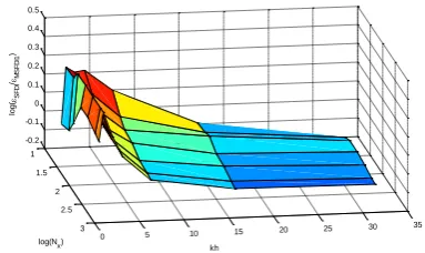
= 2π (Fig.5(b)) and 1(Fig.5(a)), respectively. For such fine particle resolution in Fig. 5(b), the exponential or the hyperbolic vertical distribution can be well approximated by using linear function, eliminating the difference between SFDI and MSFDI, as discussed in the introduction. It is expected that as the further increase of the wave number, the difference between the MSFDI and the SFDI shall keep decreasing to zero. This is confirmed by Fig. 6 which illustrates the ratio of the error for SFDI to that for MSFDI in the cases with different kh, ranging from 0.5 to 10π. In this figure, the value of log(SFDI/MSFDI)is given. A positive
value representing a increase of the accuracy. Only the results by MSFDI_1 are plotted for demonstration. One may also notice from Fig. 6 that the MSFDI is the most effective when kh around 1. As the decrease of kh from 1, the ratio and therefore the difference between SFDI and MSFDI decreases.
Figure 6: log(SFDI/MSFDI) for free surface
velocity estimations for nonlinear regular waves ka = 0.2 in the cases with different kh(quasi-uniform distribution, Nl= 2, k)
1.4 1.6 1.8 2 2.2 2.4 2.6 2.8 3
-6 -5 -4 -3 -2 -1 0
log(Nx)
lo
g
(
)
(a) kh=1 Free-surface particles
SFDI Linear MLS
MSFDI-1 w(1,2,3)
MSFDI-1 w(x,y,z)
MSFDI-2 w(1,2,3)
MSFDI-2 w(x,y,z)
1.4 1.6 1.8 2 2.2 2.4 2.6 2.8 3
-6 -5 -4 -3 -2 -1 0
log(Nx)
lo
g
(
)
(b) kh=2 Free-surface particles
SFDI Linear MLS
MSFDI-1 w(1,2,3)
MSFDI-1 w(x,y,z)
MSFDI-2 w(1,2,3)
MSFDI-2 w(x,y,z)
1
1.5
2
2.5
3
0 5 10 15 20 25 30 35
-0.2 -0.1 0 0.1 0.2 0.3 0.4 0.5
kh
log(Nx)
lo
g
(S
F
D
I
/M
S
F
D
I1
[image:10.595.81.268.302.607.2] [image:10.595.319.511.568.682.2]3.1.2 Exponential particle distribution
Investigations are also carried out on the exponential distribution of the particles, where particles are distributed in horizontal direction with even space of λ/ Nx and Eq. (9) is used to
specify the vertical distribution. Different values of Nx and Nz are used. Similar to Figs.
3-6, two layers of neighbours are used to form the support domain in this test.
Figure 7: Convergent rate for gradient estimation at free surface particles for kh =10π (exponential distribution, ka = 0.2, Nl = 2,
k
)
The first case discussed here is that with kh = 10π, a case with deep water. For such case, as discussed following Fig. 6, if a quasi-uniform particle distribution is used, the MSFDI does not show much superiority over the SFDI in terms of accuracy for specific particle resolution due to a very fine vertical particle distribution, e.g. Nz 150, corresponding to Nx
=30, in this case. In fact, such fine vertical particle distribution is unnecessary for achieving convergent solution. As indicated before, in the FNPT based QALE-FEM, 14~20 vertical layers following the exponential distribution are sufficient for achieving convergent FEM solution to the velocity potential of non-breaking extreme waves in finite depth. Unnecessary increasing the vertical particle distribution obviously leads to excessive reduction of the overall computational efficiency. Considering this, the range of Nz is taken as [5,40] in the
investigation.
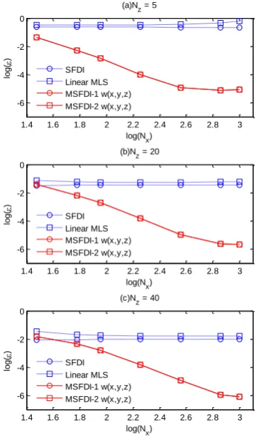
The convergent rates for gradient estimation at free surface particles in this case are illustrated in Fig. 7, together with the results from the MLS for comparison. It is observed that within the range of Nz , the MSFDI leads to
considerably higher accuracy than the SFDI, except in the cases with small Nx ,e.g. 30.
Providing a sufficient large Nx, e.g. Nx = 90, the
improvement of the accuracy compared with the SFDI may be 10 times. Fig.7 also shows that the convergent rate of the MSFDI, in particular for large kh, seems to be less sensitive to the change of Nz compared with
SFDI and the MLS. It is clearer in Fig.8 which compares the corresponding results with different Nz.
For all values of kh considered here, the results by MSFDI do not change as significantly as those by SFDI and MLS with the change of Nz.
This implies that the convergent rate and the accuracy of the MSFDI are more independent of Nz compared to others. This may be regarded
as an advantage of the MSFDI. In wave modelling practices, one may only need to consider the horizontal particle resolution or mesh sizes per wave length when investigating the convergence. Based on the results presented above, it may be deduced that, for specific Nx, the MSFDI may well reserve the
accuracy in case that the vertical particle/node
1.4 1.6 1.8 2 2.2 2.4 2.6 2.8 3 -6
-4 -2 0
log(Nx)
lo
g
(
)
(a)Nz = 5
SFDI Linear MLS MSFDI-1 w(x,y,z) MSFDI-2 w(x,y,z)
1.4 1.6 1.8 2 2.2 2.4 2.6 2.8 3 -6
-4 -2 0
log(Nx)
lo
g
(
)
(b)Nz = 20
SFDI Linear MLS MSFDI-1 w(x,y,z) MSFDI-2 w(x,y,z)
1.4 1.6 1.8 2 2.2 2.4 2.6 2.8 3 -6
-4 -2 0
log(Nx)
lo
g
(
)
(c)Nz = 40
[image:11.595.80.267.252.568.2]resolution is not as high as the horizontal direction. It is a particularly important feature for the extreme wave modelling, in which the rising free surface leads to considerable reduction of the particle/mesh resolution near the free surface.
Figure 8: Convergent rates for gradient estimation at free surface particles with different Nz(exponential distribution, ka = 0.2,
Nl= 2, k)
3.1.3 Effects of Nl
As mentioned above, another important factor related to the accuracy or the convergent rate is
the size of the support domain. In this investigation, different layers of neighbour particles (Nl), ranging from 1 to 3, are used to
test the effect of Nl.
Figure 9: Convergent rate of gradient estimation on the free surface in terms of Nl(Quasi-uniform distribution, ka = 0.2, k)
Fig. 9 displays the convergent rate for the nonlinear wave cases (ka = 0.2), in which a quasi-uniform distribution of the particle is employed. It is found that both the MSFDI and SFDI behave similarly when Nl changes, i.e.
the accuracy is improved as Nl decreases.
Especially, when Nl = 1, the MSFDI shows a
most significant improvement of the accuracy compared to the SFDI and the MLS.
It is also valuable to know whether similar conclusion may be drawn for the cases where the particles are distributed exponentially in the vertical direction. For this purpose, the corresponding results on the free surface are plotted in Fig. 10. It is found that the error of the MSFDI with Nl = 1 does not show a
continuously decreasing trend as other Nl. For
cases with different Nz, there are turning points,
e.g. Nx = 60, 90 and 180 for Nz = 10 (Fig.10(a)),
20 (Fig.10(b)) and 40 (Fig.10(c)), respectively, at which a slight increase of the error as found.
0.5 1 1.5 2 2.5 3
-7 -6 -5 -4 -3 -2 -1 0
log(Nx)
lo
g
(
)
(a) kh = 10 MSFDI-2 Nz=5
MSFDI-2 Nz=20 MSFDI-2 Nz=40 SFDI N
z=5
SFDI Nz=20 SFDI N
z=40
MLS Nz=5 MLS Nz=20 MLS Nz=40
0.5 1 1.5 2 2.5 3
-7 -6 -5 -4 -3 -2 -1 0
log(Nx)
lo
g
(
)
(b) kh = 2 MSFDI-2 N
z=5
MSFDI-2 Nz=20 MSFDI-2 N
z=40
SFDI Nz=5 SFDI Nz=20 SFDI Nz=40 MLS Nz=5 MLS Nz=20 MLS Nz=40
0.5 1 1.5 2 2.5 3
-7 -6 -5 -4 -3 -2 -1 0
log(Nx)
lo
g
(
)
(c) kh=2 MSFDI-2 Nz=5
MSFDI-2 Nz=20 MSFDI-2 Nz=40 SFDI Nz=5 SFDI Nz=20 SFDI Nz=40 MLS Nz=5 MLS N
z=20
MLS Nz=40
0.5 1 1.5 2 2.5 3
-7 -6 -5 -4 -3 -2 -1 0
log(N
x)
lo
g
(
)
(d) kh=1 MSFDI-2 Nz=5
MSFDI-2 N
z=20
MSFDI-2 Nz=40 SFDI Nz=5 SFDI N
z=20
SFDI Nz=40 MLS N
z=5
MLS Nz=20 MLS N
z=40
1.4 1.6 1.8 2 2.2 2.4 2.6 2.8 3
-10 -9 -8 -7 -6 -5 -4 -3 -2 -1
log(Nx)
lo
g
(
)
(a) kh=1
MSFDI-2 Nl=1
MSFDI-2 Nl=2
MSFDI-2 Nl=3
SFDI Nl=1
SFDI Nl=2
SFDI Nl=3
Linear MLS Nl=1
Linear MLS Nl=2
Linear MLS Nl=3
1.4 1.6 1.8 2 2.2 2.4 2.6 2.8 3
-10 -9 -8 -7 -6 -5 -4 -3 -2 -1
log(Nx)
lo
g
(
)
(b) kh=2
MSFDI-2 Nl=1
MSFDI-2 Nl=2
MSFDI-2 Nl=3
SFDI Nl=1
SFDI Nl=2
SFDI Nl=3
Linear MLS Nl=1
Linear MLS Nl=2
[image:12.595.326.507.149.372.2] [image:12.595.84.267.183.639.2]After the turning points, the error decreases as Nx increases. After the turning points, one may
see that the errors of the MSFDI with Nl = 1
may be larger than those with Nl = 2 or 3.
Before the turning points, the accuracy of the MSFDI increase as Nl decreases, consistent
with the observation in the cases with quasi-uniform distribution. By using Nl = 1, the
MSFDI leads to better accuracy than the SFDI and the MLS. Considering the FNPT modelling practices discussed above, the general requirement on the mesh resolutions to achieve convergent solution of the velocity potential are Nx ranging from 30 to 60 and Nz ranging from
14 to 20. Within this range, MSFDI with Nl = 1
leads to better estimation of the free surface velocity than the SFDI and MSFDI with other values of Nl. Similar phenomenon is also found
in the cases with other wave numbers. The results are not shown here to save the space.
Figure 10: Convergent rate of gradient estimation on the free surface in terms of Nl
(exponential distribution, ka = 0.2, kh = 2π, k
)
Figure 11: Convergent rate of gradient estimation on the free surface in terms of γ in the cases with quasi uniform distribution (ka = 0.2, Nl= 1)
Figure 12: Convergent rate of gradient estimation on the free surface in terms of γ in the case with exponential distribution (ka = 0.2, Nl= 1, Nz= 20)
1.4 1.6 1.8 2 2.2 2.4 2.6 2.8 3
-9 -8 -7 -6 -5 -4 -3 -2 -1
log(Nx)
lo
g
(
)
(a) Nz=10
MSFDI-2 Nl=1
MSFDI-2 Nl=2
MSFDI-2 Nl=3
SFDI Nl=1
SFDI Nl=2
SFDI Nl=3
Linear MLS Nl=1
Linear MLS Nl=2
Linear MLS Nl=3
1.4 1.6 1.8 2 2.2 2.4 2.6 2.8 3
-10 -9 -8 -7 -6 -5 -4 -3 -2 -1
log(Nx)
lo
g
(
)
(b) Nz=20
MSFDI-2 Nl=1
MSFDI-2 Nl=2
MSFDI-2 Nl=3
SFDI Nl=1
SFDI Nl=2
SFDI Nl=3
Linear MLS Nl=1
Linear MLS Nl=2
Linear MLS Nl=3
1.4 1.6 1.8 2 2.2 2.4 2.6 2.8 3
-10 -9 -8 -7 -6 -5 -4 -3 -2 -1
log(Nx)
lo
g
(
)
(c) Nz=40
MSFDI-2 Nl=1
MSFDI-2 Nl=2
MSFDI-2 Nl=3
SFDI Nl=1
SFDI Nl=2
SFDI Nl=3
Linear MLS Nl=1
Linear MLS Nl=2
Linear MLS Nl=3
1.4 1.6 1.8 2 2.2 2.4 2.6 2.8 3 -7
-6 -5 -4 -3 -2
log(Nx)
lo
g
(
)
(a) kh=1
MSFDI-2 2k MSFDI-2 k MSFDI-2 0.25k MSFDI-2 0.1k SFDI
1.4 1.6 1.8 2 2.2 2.4 2.6 2.8 3 -7
-6 -5 -4 -3 -2
log(Nx)
lo
g
(
)
(b) kh=2
MSFDI-2 2k MSFDI-2 k MSFDI-2 0.25k MSFDI-2 0.1k SFDI
1.4 1.6 1.8 2 2.2 2.4 2.6 2.8 3 -7
-6 -5 -4 -3 -2
log(Nx)
lo
g
(
)
(a)kh=1
MSFDI-2 2k MSFDI-2 k MSFDI-2 0.25k MSFDI-2 0.1k SFDI
1.4 1.6 1.8 2 2.2 2.4 2.6 2.8 3 -7
-6 -5 -4 -3 -2
log(Nx)
lo
g
(
)
(b) kh=2
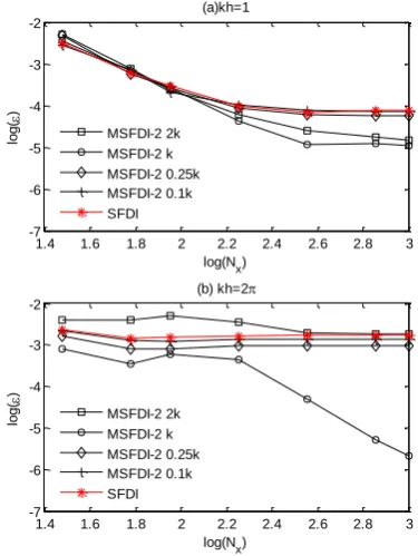
[image:13.595.318.507.113.365.2] [image:13.595.85.267.400.737.2] [image:13.595.319.507.444.694.2]3.1.4 Effects of γ
In the results shown above, k is taken in Eq. (2). This is a reasonable for regular waves, however, it is important to see how the accuracy and the convergent rate of the MSFDI are affected by different values of . Such
investigation will shed a light for the assignment of in the cases with wave groups
consisting of many wave components. For this purpose, different ranging from 0.1k to 10k,
are used for each cases with different wave numbers. Two typical examples are illustrated in Fig. 11 and Fig.12, for quasi-uniform particle distribution and exponential particle distribution, respectively, in which ka = 0.2, Nl= 1 are used.
These figures show that when γ is taken as a value too smaller than the wave number k, the accuracy of the MSFDI for specific particle resolution decreases to that of the SFDI at γ =0.1k. On the other hand, the accuracy of the MSFDI is more sensitive to the value of γ when it is assigned a value greater than k. It is generally seen that if γ is greater than 2k, the MSFDI loss its superiority over the SFDI. A similar phenomenon is also observed in the cases with other wave steepness, wave numbers, Nl and Nz. Based on the investigation, the
reasonable range for γ is 0.1k ~ 2k.
3.2 Wave groups
In this section, the comparison between the MSFDI and other schemes are made using the cases with wave groups. Both the random sea state and the focusing wave groups are considered here. Although other parameters have been tested, only MSFDI-2 with Nl = 1
and exponential particle distribution are presented in this section.
In the first case, we consider a focusing wave group generated using the spatial-temporal
focusing mechanism which has been used both experimentally and numerically as reviewed by Ma (2007) in a water depth h = 10m. 64 wave components with frequencies at equally spaced
from h/g to 3 h/g. Each wave component
is assigned the same wave amplitude, i.e. 0.00225h. Their phases are carefully selected to ensure their crests focus at the focusing point xf
at the focusing time, leading to a giant wave. The 2nd order wave theory (Schaffer, 1996; Toffoli, Onotato, Babanin, Bitner-Gregersen, Osborne and Monbaliu, 2007) is used here to provide the analytical results of the wave elevation, velocity potential and the velocity. At the focusing time, the local wave steepness H/λ, where H is the wave height, is about 0.2 and the local wave number kh ≈ 2π. For such simplified spectrum where each component contains equal energy, γ is taken as the wave number corresponding to the midpoint of the frequency range (refer to kavg). The
computational domain is taken as 10h surrounding the focusing point.
Figure 13: Convergent rate of gradient estimation on the free surface for focusing waves (frequency range h/g ~ 3 h/g , Exponential particle distribution MSFDI-2 with Nl = 1, Nz = 20)
Fig.13 displays the convergent rate of gradient estimation at free-surface particles using the velocity potential given by the 2nd order wave theory in the cases with exponential particle distribution and Nz = 20. As expected, the
errors of all schemes approach a steady value as Nx increases and the MSFDI lead to the best
accuracy. In the case with convergent solution, e.g. Nx =6400(log(Nx)≈3.8), the relative error of
1.5 2 2.5 3 3.5 4 4.5 -3
-2 -1 0
log(Nx)
lo
g
(
)
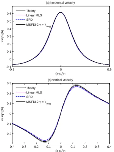
the MSFDI is around 0.6 of those of SFDI and linear MLS. In order to show how the error distributed spatially, the free surface velocities near the crest are compared in Fig.14, which demonstrates that the results by the MSFDI agree with the theoretical solution better than the SFDI and the MLS, particularly the vertical velocity near the wave crest which is the most critical in the focusing wave simulation. It should be noted that Fig. 14 only demonstrates the error at one time step. During the time-domain simulation, the error at every time step may be accumulated, resulting in a significant overall error after long time simulation, as indicated before. The overall error by these gradient estimation schemes in a time domain simulation will be discussed in Section 5.
Figure 14: Free surface velocity near the crest at the focusing time (frequency range h/g ~
3 h/g ; Exponential particle distribution MSFDI-2 with Nl = 1, Nz = 20, Nx = 6400)
Although such simplified spectrum is commonly used in the experimental and numerical simulation, it is rarely seen in real scenario. Another case in finite water with real spectrum is discussed below. In this case, an
event similar to the ‘New Year Wave’ recorded at the Draupner platform in the North Sea, a rare high-quality measurement of a ‘freak’ or ‘rogue’ wave, on 1st
January 1995. The local water depth at the site is about 70m and the giant wave had a crest of mean 18.6 m above mean see level and was 25.6 m in height. A JONSWAP spectrum with a peak at around 0.067 Hz may be used to describe this event (Adcock, Taylor, Yan, Ma and Janssen, 2011; Adcock and Taylor, 2014). The wave number near the crest kh is about 1.6, a typical focusing wave in finite water depth. Again, 2nd order wave theory is used to provide the analytical solutions. It should be noted that this event may be caused by two directional wave groups crossing in the sea (Adcock, Taylor, Yan, Ma and Janssen, 2011). However, 2D simplification is considered here. This may not well re-produce the event but provides sufficiently good data for the convergence test. The computational domain covers 700m around the crest (x = xf). The corresponding convergent
rates on the free surface velocity estimation near the focusing crest at the focusing time are displayed in Fig.15. Similar to those in Fig.13, the results of the MSFDI with γ being the wave number corresponding to the significant wave converge to results with small error using less number of particles compared to the SFDI and the MLS.
Figure 15: Convergent rate of gradient estimation on the free surface for focusing waves (JONSWAP, peak frequency 0.067Hz, Exponential particle distribution MSFDI-2 with Nl = 1, Nz = 20)
The third case demonstrated here is a 2D random wave group, which is generally seen in
-0.5 0 0.5
-0.1 0 0.1 0.2 0.3 0.4 0.5 0.6
(x-xf/)h
u
/s
q
rt
(g
h
)
(a) horizontal velocity Theory
Linear MLS SFDI MSFDI-2 = kavg
-0.4 -0.3 -0.2 -0.1 0 0.1 0.2 0.3 0.4 -0.2
-0.1 0 0.1 0.2 0.3
(x-x
f/)h
w
/s
q
rt
(g
h
)
(b) vertical velocity Theory
Linear MLS SFDI MSFDI-2 = k
avg
2 2.5 3 3.5 4
-3.5 -3 -2.5 -2
log(N
x)
lo
g
(
)
[image:15.595.79.271.342.599.2] [image:15.595.315.508.563.661.2]reality. In this case, JONSWAP spectrum with peak period of 12.5s and significant wave height H1/3 of 12m are used. The water depth is
70m. This is a typical sea state in North Sea. In the test, the length of the computational domain is 4000m. Exponential particle distribution with Nz = 20 are used to generate the particles. Nl = 1
is used for all gradient estimation schemes. γ in the MSFDI is taken as the wave number corresponding to the significant wave.
Figure 16: Free surface elevation and velocity in random sea (JONSWAP, h = 70m, peak period 12.5s, H1/3 = 12m, Exponential particle
distribution MSFDI-2 with Nl = 1, Nz = 20)
Figure 17: Convergent rate of gradient estimation on the free surface in random sea (JONSWAP, h = 70m, peak period 12.5s, H1/3 =
12m, Exponential particle distribution MSFDI-2 with Nl = 1, Nz = 20)
Fig. 16(a) illustrates the free surface elevation at one time instant obtained by using 2nd order
wave theory. Fig. 16(b) and (c) compares the analytical and the MSFDI solutions to the velocity at the free surface particles at the same instant, where Nx = 6400, i.e. log(Nx)≈3.8, is
used by the MSFDI. A satisfactory agreement has been observed. The relative errors for the free surface velocity estimation in terms of horizontal particle resolution are plotted in Fig. 17, together with the corresponding results by other scheme. Again, the MSFDI shows its superiority over the SFDI and MLS in terms of accuracy or convergent rate.
5. Implementation of MSFDI in QALE-FEM modelling
Figure 18: Sketch of the wave flume at the Harbin Engineering University, China
In this section, the MSFDI is implemented by the QALE-FEM method for time-domain nonlinear wave simulations. For validation purpose, experiments have been carried out in the wave flume at the Harbin Engineering University, China. The sketch of the flume is given in Fig. 18. The mean water depth is 3.5m and the total length of the flume is 108m. A hinged wavemaker is installed at the left end of the flume with rotational centre located at 1.64m above the bed. An absorbing beach is used to absorb the wave in the end of the wave flume. The numerical simulation is carried out in a numerical wave tank with the same dimension. A Sommefeld condition together with a damping zone is employed in the right end of the numerical tank to absorb the wave. Various wave gauges are installed to measure the time histories of the wave elevations. Both SFDI and MSFDI with Nl = 1 are used in the
0 500 1000 1500 2000 2500 3000 3500 4000 -10
-5 0 5 10
x(m)
(
m
)
(a) free surface elevation
0 500 1000 1500 2000 2500 3000 3500 4000 -6
-4 -2 0 2 4 6
x(m)
u
(m
/s
)
(b) horizontal velocity
Theory
MSFDI-2 = ksig Nx = 6400
0 500 1000 1500 2000 2500 3000 3500 4000 -6
-4 -2 0 2 4 6
x(m)
w
(m
/s
)
(c) vertical velocity
Theory
MSFDI-2 = ksig, Nx = 6400
2.4 2.6 2.8 3 3.2 3.4 3.6 3.8 -4
-3 -2 -1 0
log(N
x)
lo
g
(
)
SFDI Linear MLS MSFDI-2 = k
sig
3
.5
108
1
.6
4
[image:16.595.84.272.239.484.2] [image:16.595.321.509.323.413.2] [image:16.595.82.265.551.650.2]QALE-FEM to estimate the free surface velocity.
[image:17.595.82.269.349.422.2]Figure 19: Comparison of the time histories of the wave elevations recorded at the gauge with the experimental data (Nl = 1, Nz = 20)
Figure 20: Comparison of the time histories of the wave elevations recorded at the gauge with the three-point finite difference scheme
The first case considered here is a regular wave with wave period of 2s and wave height of 0.12m. A linear wavemaker theory is used to configure the wavemaker motion. A wave gauge located at 15m from the wavemaker is applied to record the time history of the wave elevation. In the QALE-FEM, the initial mesh is generated with Nz = 20 and different values
of dx on the free surface ranging from λ/30 to λ/60 are used, corresponding to Nx = 30 to 60
per wave length. The time step is taken as T/200 where T is the wave period. The wavemaker motion used in the QALE-FEM is specified to be the same as those in the physical experiments.
Fig.19 displays the time histories of the wave elevations recorded at the wave gauge. It is found from Fig. 19(a) that the results from the
MSFDI with Nx = 30 agree well with the
experimental results. The relative error on the wave elevation, which is evaluated using Eq.(10) with velocities being replaced by corresponding wave elevation, is less than 0.1%; whereas the SFDI leads to not only slightly smaller wave amplitude but also a considerably phase shift. This suggests that Nx = 30 is not
sufficiently large for SFDI to achieve convergent results, as confirmed by Fig. 19(b) where Nx = 60 is used and the results with SFDI
agree with the experimental data better than those in Fig. 19(a). This suggests that the MSFDI has better convergent property than the SFDI when implemented in the QALE-FEM. To achieve the convergent results, the SFDI needs half of the horizontal free surface mesh size than the MSFDI. As a result, the CPU time spent by the QALE-FEM with SFDI is almost the double of that by the QALE-FEM with MSFDI. Comparison with the three-point finite difference scheme suggested by Ma and Yan (2006) has also been made. It concludes that the MSFDI leads to a similar accuracy level to the three-point scheme for specific mesh size, as demonstrated by Fig. 20 where Nx= 30 are
used. However, the CPU time spent on the free surface velocity estimation by the MSFDI is about 1/10 of that by the three-point scheme, yielding a total reduction on the CPU time of about 1/4 to achieve the results shown in Fig. 20.
The experiments in the same flume on the focusing wave group are also used for validation purpose. In this case, the spatial-temporal focusing mechanism used by Ma (2007) is considered here. 32 wave components with wave period ranging from 1.7s to 4.7s, are used in both the experiment and the numerical simulation. The focusing point and the focusing time are specified at 30m and 36s, respectively. A linear wavemaker theory is used to specify the phases for each wave components, yielding an expected crest 0.1m above the mean free
30 32 34 36 38 40 42 44 46 48 50 -0.05
0 0.05
(a)Nx = 30, Nz = 20
time(s)
(m
)
experimental MSFDI-2 SFDI
30 32 34 36 38 40 42 44 46 48 50 -0.05
0 0.05
(b)Nx = 60, Nz = 20
time(s)
(m
)
experimental MSFDI-2 SFDI
0 10 20 30 40 50 60
-0.05 0 0.05
time(s)
(m
)
surface when the wave group focuses. The details can be found at Ma (2007). It is noted that the wavemaker motion specified using the linear theory may lead to a significant shift of the focusing point caused by the interactions between the progressive waves, wavemaker motion and the evanescent waves (Schaffer, 1996). In order to well capture the focusing point, 24 wave gauges installed near the expected focusing point are used in the investigation.
Figure 21: Comparison of the time histories of the wave elevations for focusing wave group (dx = 0.2m, Nl = 1, Nz = 20)
Fig.21 compares the time histories of the wave elevations recorded at different locations in the cases with dx = 0.2m and Nz = 20. In the
MSFDI and SFDI, Nl= 1 is used. To save the
space, only the results at three gauges, i.e. one in front of (Fig.21(a)), one at (Fig.21(b)) and one behind the actual focusing point (Fig.21(c)). Again, both the results obtained using MSFDI and three-point scheme agree well with the experimental. But the former spends about ¾ overall CPU time of the latter. It is also found
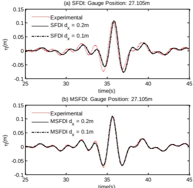
that the results from the QALE-FEM with SFDI considerably different from the experimental data for the mesh used here, although the CPU time is at the same level as the MSFDI. By reducing the mesh size, dx, the results by the QALE-FEM with SFDI do not seem to change, as shown in Fig.22 (a), suggesting that SFDI leads to convergent solutions with lower accuracy than the convergent solutions by the MSFDI which are demonstrated in Fig.22(b). This is consistent with conclusions obtained from Figs. 13 and 15.
Figure 22: Comparison of the time histories of the wave elevations at x = 27.105m (Nl= 1, Nz
= 20)
6. Conclusion
In this paper, a modified SFDI (MSFDI) scheme is developed based on the SFDI scheme for the gradient estimation and investigated using the fully nonlinear water wave problems. The modification takes into account of the feature of the vertical variation of the wave-related parameters. Based on the numerical tests, one observes the following features: (1) The MSFDI is generally more accurate than the SFDI and the linear MLS for the estimating free surface velocity, particularly when an exponential particle distribution is used; (2) The MSFDI is less sensitive to the vertical particle/node distribution; (3) In the
QALE-25 30 35 40 45
-0.1 -0.05 0 0.05 0.1 0.15
time(s)
(m
)
(a)Gauge Position: 21.905m
Experimental MSFDI-2 SFDI 3-point
25 30 35 40 45
-0.1 -0.05 0 0.05 0.1 0.15
time(s)
(m
)
(b)Gauge Position: 27.105m
Experimental MSFDI-2 SFDI 3-point
25 30 35 40 45
-0.1 -0.05 0 0.05 0.1 0.15
time(s)
(m
)
(c)Gauge Position: 29.105m
Experimental MSFDI-2 SFDI 3-point
25 30 35 40 45
-0.1 -0.05 0 0.05 0.1 0.15
time(s)
(m
)
(a) SFDI: Gauge Position: 27.105m
Experimental
SFDI dx = 0.2m
SFDI dx = 0.1m
25 30 35 40 45
-0.1 -0.05 0 0.05 0.1 0.15
time(s)
(m
)
(b) MSFDI: Gauge Position: 27.105m
Experimental
MSFDI dx = 0.2m
[image:18.595.314.507.280.468.2]FEM practices, the MSFDI leads to similar convergent property as the three-point scheme but better than the SFDI; (4) the CPU time required by the MSFDI to achieve convergent results is about half of that by the SFDI and 3/4 of that by the three-point method. Although only the application on the mesh based QALE-FEM is presented, the preliminary investigation on the quasi-uniform particle distribution reveals the superiority of MSFDI over the SFDI and linear MSL when being implemented by meshless methods, e.g. the MLPG_R method.
Acknowledgement: The first author is
supported by the Chinese Scholarship Council, to which the author is most grateful. UK authors acknowledge the financial support from the ESPRC, UK (EP/L01467X/1).
Reference
Adcock, T.A.A; Taylor, P.H.(2014): The
physics of anomalous (‘rogue’) ocean waves, Reports on Progress in Physics, Vol. 77, 105901.
Adcock, T.A.A; Taylor, P.H.; Yan, S.; Ma,
Q.W.; Janssen, P.A.E.M. (2011): Did the
Draupner wave occur in a crossing sea? Proceeding of the Royal Society A, doi:10.1098/rspa.2011.0049.
Atluri, S.N.; Shen, S. (2002): The Meshless Local Petrov-Galerkin (MLPG) Method: A Simple & Less-costly Alternative to the Finite Element and Boundary Element Methods, CMES: Computer Modeling in Engineering & Sciences, Vol. 3(1), pp. 11-52.
Atluri, S.N.; Zhu, T. (1998): A New Meshless
Local Petrov-Galerkin (MLPG) approach in Computational Mechanics, Computational Mechanics, Vol. 22, pp. 117-127.
Dalzell, J.F. (1999): A note on finite depth second-order wave-wave interactions, Applied Ocean Research, Vol. 21, pp. 105-111.
Fochesato, C.; Dias, F.(2006), A fast method for nonlinear three-dimensional free-surface
waves. Proceedings of the Royal Society of London, Series A, Vol. 462, pp. 2715–2735.
Fenton, J. (1985): A Fifth-Order Stokes
Theory for Steady Waves, Journal of Waterway, Port, Coastal and Ocean Engineering, Vol. 111(2), pp. 216-234.
Koshizuka S.; Oka, Y. (1996):
Moving-Particle Semi-Implicit Method for Fragmentation of Incompressible Fluid, Nuclear Science and Engineering, 123, pp.421-434.
Ma, Q.W. (2005): MLPG Method Based on
Rankine Source Solution for Simulating Nonlinear Water Waves, CMES: Computer Modeling in Engineering & Sciences, Vol9(2), pp. 193-210.
Ma, Q.W. (2007): Numerical generation of freak waves using MLPG_R and QALE-FEM methods. CMES: Computer Modeling in Engineering & Sciences, Vol. 18(3), 223-234
Ma, Q.W. (2008): A New Meshless Interpolation Scheme for MLPG_R Method, CMES: Computer Modeling in Engineering & Sciences, Vol. 23(2), pp. 75-89.
Ma, Q.W.; Wu, G.X.; Eatock Taylor, R.(2001): Finite element simulation of fully non-linear interaction between vertical cylinders and steep waves. Part 1: methodology and numerical procedure, International Journal for Numerical Methods in Fluids, Vol. 36(3):265–285.
Ma, Q.W.; Yan, S.(2006): Quasi ALE finite element method for nonlinear water waves, Journal of Computational Physics, Vol. 212,pp. 52–72.
Schaffer, H.A. (1996): Second-order
wavemaker theory for irregular waves, Ocean Engineering, Vol. 23, pp.47-88.
Sriram, V.; Ma, Q.W.(2012): Improved
MLPG_R method for simulating 2D interaction between violent waves and elastic structures, Journal of Computational Physics, Vol.231, pp. 7650-7670.
Sriram, V.; Ma, Q.W.(2014): A Hybrid