City, University of London Institutional Repository
Citation
:
Bleisch, S. (2011). Evaluating the appropriateness of visually combining
quantitative data representations with 3D desktop virtual environments using mixed
methods. (Unpublished Doctoral thesis, City University London)
This is the unspecified version of the paper.
This version of the publication may differ from the final published
version.
Permanent repository link: http://openaccess.city.ac.uk/1092/
Link to published version
:
Copyright and reuse:
City Research Online aims to make research
outputs of City, University of London available to a wider audience.
Copyright and Moral Rights remain with the author(s) and/or copyright
holders. URLs from City Research Online may be freely distributed and
linked to.
d
Evaluating the appropriateness of visually combining
quantitative data representations with
3D desktop virtual environments
using mixed methods
Susanne Barbara Bleisch
Thesis Submission for Admission to degree of Doctor of Philosophy in Geographic Information Science
City University London Information Science
Contents
Contents 2
List of Tables 7
List of Figures 8
Acknowledgements 14
Abstract 16
1. Introduction 18
1.1. Virtual Globes - the past and the present . . . 20
1.2. Motivation and background. . . 21
1.2.0.1. Geodata availability . . . 21
1.2.0.2. Geovisualization . . . 21
1.2.0.3. Virtual environments . . . 22
1.2.1. Categorisation and examples of 3D representations and applications . . . 22
1.2.1.1. Examples for 1) - focus on data . . . 23
1.2.1.2. Examples for 2) - focus on depicting the real world . . . 25
1.2.1.3. Examples for 3) - combination of data and real world representation . 25 1.2.1.4. Discussion . . . 25
1.2.2. Evaluations of 3D representations and applications. . . 27
1.2.3. Review of research agendas . . . 32
1.3. Problem statement. . . 33
1.4. Aims and research questions . . . 36
1.4.0.1. Research questions . . . 36
1.4.0.2. Hypotheses . . . 36
1.5. Summary of contributions. . . 38
2. Methods 40 2.1. Methodological overview of the research. . . 41
2.1.0.1. Representations of quantitative data . . . 42
2.1.0.2. Measures of appropriateness . . . 42
2.1.0.3. Evaluation methods . . . 43
2.1.0.4. Overview of research stages. . . 44
2.2. Defining tasks. . . 47
2.3. Data representation . . . 48
2.3.1. Data graphics design . . . 48
2.3.2. Preparation of 2D and 3D visualisations. . . 50
2.5. Research methods and implementation . . . 52
2.5.1. Stage I . . . 52
2.5.1.1. Method. . . 52
2.5.1.2. Tasks. . . 52
2.5.1.3. Data set . . . 53
2.5.1.4. Implementation . . . 53
2.5.1.5. Collected data . . . 55
2.5.2. Stage IIa . . . 55
2.5.2.1. Method. . . 56
2.5.2.2. Tasks. . . 56
2.5.2.3. Data set . . . 58
2.5.2.4. Implementation . . . 58
2.5.2.5. Collected data . . . 59
2.5.3. Stage IIb . . . 60
2.5.3.1. Method. . . 60
2.5.3.2. Tasks. . . 60
2.5.3.3. Data set . . . 60
2.5.3.4. Implementation . . . 61
2.5.3.5. Collected data . . . 62
2.5.4. Stage III . . . 62
2.5.4.1. Method. . . 62
2.5.4.2. Tasks. . . 63
2.5.4.3. Data sets . . . 63
2.5.4.4. Implementation . . . 64
2.5.4.5. Collected data . . . 64
2.6. Analysing the data . . . 67
2.6.1. Quantitative analysis methods . . . 67
2.6.1.1. Analysing time data . . . 67
2.6.1.2. Analysing bar length comparison data . . . 67
2.6.1.3. Analysing categorical data . . . 67
2.6.2. Qualitative analysis methods . . . 67
2.6.2.1. Analysing insights for complexity and plausibility . . . 68
2.6.2.2. Process of manual coding . . . 69
2.6.2.3. Analysing insights for reference type . . . 70
2.6.2.4. Analysing word counts . . . 70
2.6.2.5. Analysing case study data . . . 70
2.6.2.6. Analysing participants comments . . . 71
2.6.2.7. Analysing think-aloud reports . . . 72
2.6.3. Data handling . . . 72
2.6.3.1. Stage I . . . 72
2.6.3.2. Stage IIa. . . 73
2.6.3.3. Stage IIb. . . 73
3. Data analysis and results 75
3.1. Stage I - Evaluating single bars with simple tasks . . . 75
3.1.1. Description of the sample . . . 75
3.1.1.1. Time . . . 76
3.1.1.2. Bar length differences . . . 76
3.1.1.3. Identification of the taller bar . . . 76
3.1.1.4. Estimating absolute bar lengths . . . 77
3.1.2. Testing research hypotheses . . . 77
3.1.3. Further analysis of the data . . . 78
3.2. Stage IIa - Evaluating single bars with more complex tasks . . . 78
3.2.1. Description of the sample . . . 78
3.2.1.1. Time . . . 78
3.2.1.2. Confidence rating . . . 79
3.2.1.3. Complexity . . . 79
3.2.1.4. Plausibility. . . 79
3.2.1.5. Word count analysis . . . 80
3.2.2. Testing research hypotheses . . . 80
3.2.2.1. Hypotheses regarding efficiency . . . 80
3.2.2.2. Hypotheses regarding effectiveness . . . 81
3.2.3. Further analysis of the data . . . 83
3.2.3.1. Complexity vs. plausibility . . . 83
3.2.3.2. Task references vs. insight references . . . 83
3.2.3.3. Confidence ratings. . . 84
3.2.3.4. Differences between settings . . . 85
3.2.3.5. Differences between data sets. . . 86
3.2.3.6. Word count analysis . . . 88
3.3. Stage IIb - Evaluating bar charts with more complex tasks . . . 88
3.3.1. Description of the sample . . . 88
3.3.1.1. Time . . . 89
3.3.1.2. Confidence rating . . . 89
3.3.1.3. Complexity . . . 89
3.3.1.4. Plausibility. . . 89
3.3.1.5. Word count analysis . . . 90
3.3.2. Testing research hypotheses . . . 90
3.3.2.1. Hypotheses regarding efficiency . . . 90
3.3.2.2. Hypotheses regarding effectiveness . . . 91
3.3.3. Further analysis of the data . . . 92
3.3.3.1. Complexity vs. plausibility . . . 92
3.3.3.2. Differences between data sets and settings . . . 92
3.3.3.3. Word count analysis . . . 94
3.4. Comparing stages IIa and IIb . . . 94
3.4.0.1. Time . . . 94
3.4.0.2. Confidence . . . 94
3.4.0.3. Complexity . . . 94
3.4.0.4. Plausibility. . . 95
3.4.0.6. Word count analysis . . . 95
3.5. Stage III - Evaluating bar charts with more complex tasks and application context . . . 96
3.5.1. Data experts’ characteristics . . . 96
3.5.2. Summary of the case data. . . 96
3.5.3. Data analysis regarding the propositions and exploratory questions . . . 97
3.5.4. Further analysis of the case data . . . 103
3.6. Analysis of participant’s comments in all research stages. . . 104
3.6.1. Quantitative data graphics . . . 104
3.6.2. Tasks . . . 106
3.6.3. Visualisations, interaction and navigation . . . 106
3.6.4. Suitability . . . 107
4. Discussion 110 4.1. Summary and discussion of results and findings . . . 111
4.1.1. Quantitative data graphics . . . 112
4.1.2. Accuracy of data graphic interpretation . . . 113
4.1.3. Comparing 2D and 3D visualisations . . . 114
4.1.3.1. Overview . . . 114
4.1.3.2. Relation of data and landscape . . . 116
4.1.3.3. Summary . . . 117
4.1.4. Tasks . . . 118
4.1.5. Settings and data sets . . . 120
4.1.6. Increasing complexity - comparing stage IIa and IIb. . . 123
4.1.7. Further visualisation aspects . . . 126
4.2. Reflection on the methodological framework . . . 127
4.2.1. Summary of the research stages . . . 128
4.2.2. Employing a mixed methods approach . . . 130
4.2.3. Further methodological aspects . . . 134
4.2.4. A mixed methods approach to bridge between ’in vitro’ and ’in vivo’ . . . 136
5. Conclusions and outlook 139 5.1. Revisiting research aims and objectives . . . 140
5.2. Conclusions. . . 141
5.2.1. Concluding on the visualisations . . . 141
5.2.1.1. Data graphics. . . 141
5.2.1.2. Relation of data and landscape . . . 142
5.2.1.3. Data sets and settings . . . 142
5.2.1.4. Ancillary conclusions . . . 143
5.2.2. Concluding on the methods . . . 144
5.3. Recommendations. . . 147
5.3.1. Data displays in virtual environments . . . 147
5.3.2. Evaluation methods. . . 148
5.4. Implications . . . 151
5.5. Further research . . . 153
5.6. Outlook . . . 155
Appendices 168
A. ’The Cartographic Journal’ article (Bleisch et al. 2008) 169
B. Data sets and visualisations 181
B.1. Stage IIa: data sets and visualisations . . . 183
B.2. Stage IIa: characteristics of data sets and settings. . . 191
B.3. Stage IIb: data sets and visualisations . . . 192
B.4. Stage III: data sets and visualisations . . . 197
C. Implementation documents 203 C.1. Stage IIa . . . 203
C.2. Stage IIb . . . 206
C.3. Stage III . . . 207
List of Tables
1.1. Overview of explored and tested aims, research objectives and hypotheses . . . 37 2.1. Overview of the characteristics of each stage and the differences between the
re-search stages
(including references to the sections and figures where details are available) . . . 46 2.2. Tasks, task numbers and task references as used in stage IIa . . . 56 2.3. Overview of the characteristics of the case study areas, data sets and visualisations . 65 2.4. Explanations and examples of complexity levels for insight rating . . . 68 2.5. Word categories and respective example words (the category short names are used
in the figures in the analysis chapter 3) . . . 71 3.1. Ratings of the different measures for the comparison of the visualisations of the data
sets in 2D and 3D . . . 86 3.2. Most appropriate visualisation type per data set based on the ratings described in
table 3.1 . . . 87 3.3. Context information and descriptive case data (table data are condensed case study
data experts views or from referenced literature); table 2.3 for a general description of the cases and data sets. . . 98 3.4. The expert’s analysis and explanations of their data using the visualisations (table
data are condensed case study data experts views, researcher’s interpretations or
[explanations] are written in italic type). . . 99 3.5. Case data regarding data and visualisation use (table data are condensed case study
data experts views or from referenced literature, researcher’sinterpretations or [ex-planations] are written in italic type) . . . 100 3.6. Suitability ratings of the visualisations by the data experts (rated on a seven-point scale)101 3.7. Comparison of different performance measures for participants stating that either the
2D or the 3D visualisation is better (time: left graphic, maximum value 3D=465; right graphic, maximum values 2D=537, 3D=830) . . . 109 4.1. Tested hypothesis about the efficiency of reference frames (4= accepted,8= rejected)112 4.2. Overview of tested hypotheses about basic bar comparison in 2D and 3D (4=
accep-ted,8= rejected). . . 114 4.3. Overview of tested hypothesis about the efficiency of basic bar comparison in 2D and
3D (4= accepted,8= rejected). . . 115 4.4. Overview of tested hypothesis about complexity and plausibility of insights (4=
ac-cepted,8= rejected) . . . 115 4.5. Overview of tested hypotheses and evaluated propositions about data and landform
4.7. Overview of tested hypotheses in Stage I (4= accepted,8= rejected) . . . 128 4.8. Overview of tested hypotheses in stage IIa (4= accepted,8= rejected) . . . 129 4.9. Overview of tested hypothesis in stage IIb (4= accepted,8= rejected) . . . 129 4.10.Overview of evaluated propositions and questions in stage III (4= accepted,8=
re-jected,W= not answered) . . . 130 5.1. Overview of explored and tested aims, research objectives and main hypotheses
List of Figures
1.1. Sensor Web concept (Botts, Percivall, Reed & Davidson 2006, p. 4) . . . 22 1.2. Virtual environment showing a real landscape - view of the S ¨antis mountain in eastern
Switzerland in Google Earth (Google 2010) . . . 23 1.3. Examples of 3D representations. . . 24 1.4. Front covers of the journal Kartographische Nachrichten from mid 2008 to mid 2010 . 27 1.5. Map of the Toggenburg area showing the religion of the villages and localities (Ambroziak
& Ambroziak 1999) . . . 34 2.1. The bridge between the two sides of ’in vitro’ and ’in vivo’ research approaches . . . . 44 2.2. Functional view of a data set. A set of references (R) linked to a set of characteristics
(C) (Andrienko & Andrienko 2006, p. 7) . . . 47 2.3. Two elementary tasks represented schematically on the basis of the functional view
of data in figure 2.2 (Andrienko & Andrienko 2006, p. 8) . . . 47 2.4. Compare Switzerland (red arrow) with Albania (green arrow) from two different
view-points (children under five mortality rate, circular symbols in Google Earth; display created with thematicmapping.org/engine (Sandvik 2010)) . . . 49 2.5. Hexagonal 3D bars in Google Earth - side and top view (display created with GE-graph
(Sgrillo 2010)). . . 49 2.6. Exemplary background map (swisstopo 2010) and ortho imagery readability . . . 51 2.7. Four different settings of the 2x2 factorial design (static 2D representations without ’2D
nf’ and with frames ’2D f’ and interactive 3D desktop virtual environments containing bars without ’3D nf’ and with frames ’3D f’), figures 2.8 and 2.9 for all bar combinations C1–C20 (Bleisch, Dykes & Nebiker 2008) . . . 53 2.8. All 20 bar combinations in the ’2D f’ setting. The proportion of the smaller bar to
the taller bar is given as a percentage value (’2D nf’ setting: same bar positions but without frames) (Bleisch et al. 2008) . . . 54 2.9. All 20 bar combinations in the ’3D nf’ setting (screenshots of interactive 3D
visualisa-tions from a fixed viewpoint). The proportion of the smaller bar to the taller is given as a percentage value (’3D f’ setting: same bar positions but with frames) (Bleisch et al. 2008) . . . 55 2.10.2D and 3D representations of the different data sets (W1-W4 and S1-S4) in the two
different areas W (top half) and S (lower half); larger figures in appendix B.1 . . . 57 2.11.2D and 3D representations of the two data sets in the two different areas W and S
(one data set per area); larger figures in appendix B.3 . . . 61 2.12.Exemplary 3D representations of the different case study data sets and areas; larger
figures in appendix B.4 . . . 66 2.13.Comparison of the complexity ratings (high, medium, low) of the insights between the
2.14.Comparison of the plausibility ratings (high, medium, low) of the insights between the author (B) and researcher I in 2D and 3D . . . 69 2.15.Comparison of the complexity ratings (high, medium, low) of the insights between the
author (B) and researcher II in 2D and 3D . . . 70 2.16.Comparison of the plausibility ratings (high, medium, low) of the insights between the
author (B) and researcher I in 2D and 3D . . . 70 3.1. Mean, standard deviation (calculated from log normal distribution), and minimum/maximum
values (max value 3Dnf = 98) of task completion time in seconds in all four settings, 3 seconds of 3D scene start-up time were subtracted in the two 3D settings ’3D f’ and ’3D nf’ (Bleisch et al. 2008, p. 220,îAppendix A) . . . 76 3.2. Mean, standard deviation, and minimum/maximum values (max value 3Df = 45) of
the differences between estimated and actual values in all four settings (Bleisch et al. 2008, p. 220,îAppendix A) . . . 76 3.3. Correct and incorrect judgements of the taller bar. Medium grey values indicate bar
combinations judged as being of equal size (figure 3.4) (Bleisch et al. 2008, p. 220,î
Appendix A) . . . 76 3.4. Frequency of bar combinations judged as being of equal size (proportion of the two
bars as a percentage) (Bleisch et al. 2008, p. 220,îAppendix A) . . . 76 3.5. Mean, standard deviation, and minimum/maximum values of the differences between
recorded and absolute values when estimating absolute values (Bleisch et al. 2008, p. 221,îAppendix A) . . . 77 3.6. Mean, standard deviation (calculated from log normal distribution), and minimum/maximum
values of task completion time in seconds for estimating and recording absolute val-ues (Bleisch et al. 2008, p. 221,îAppendix A). . . 77 3.7. Boxplots of 2D (left, n=468, max value=1016) and 3D (right, n=464, max value=830)
times per answer in seconds . . . 79 3.8. Confidence ratings of answers in 2D and 3D (number of answers with low, medium
and high confidence) . . . 79 3.9. Complexity of insights in 2D and 3D (number of insights with low, medium and high
complexity) . . . 79 3.10.Plausibility of insights in 2D and 3D (number of insights with low, medium and high
plausibility) . . . 79 3.11.Word counts for the different word categories L1-L3 and A1-A3 (explained in table 2.5)
in 2D and 3D . . . 80 3.12.Boxplots of task times for different reference sets (L location, A altitude and LA both)
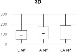
in 2D (maximum values: L=468, A=665, LA=1016) . . . 81 3.13.Boxplots of task times for different reference sets (L location, A altitude and LA both)
in 3D (maximum values: L=809, A=830, LA=619) . . . 81 3.14.Insight complexity per dimension (2D and 3D) and task reference set (L location, A
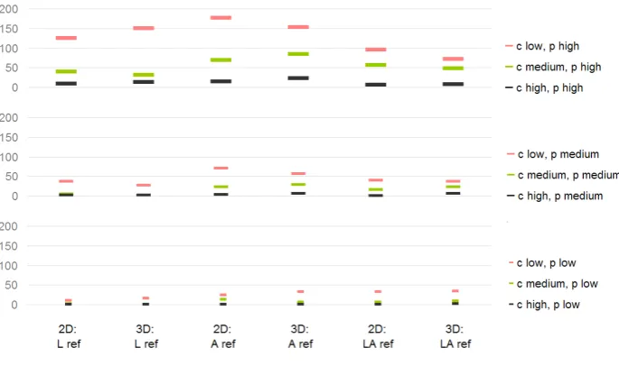
altitude and LA both) . . . 82 3.15.Insight plausibility per dimension (2D and 3D) and task reference set (L location, A
altitude and LA both) . . . 82 3.16.Numbers of insights with low, medium and high complexity, separated by task
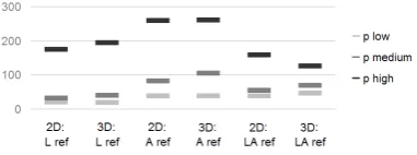
3.17.Number of insights per reference type (L location, A altitude and LA both), separated by task reference (L, A and LA) and dimension (2D and 3D) . . . 84 3.18.Confidence ratings (high, medium and low) per task reference (L location, A altitude
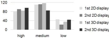
and LA both) in 2D and 3D . . . 84 3.19.Confidence ratings (high, medium and low) per per first and second displays in 2D
and 3D . . . 84 3.20.Boxplot of times for the two environmental settings (W and S) in 2D and 3D (maximum
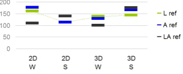
values: 2D W=665, 2D S=1016, 3D W=830, 3D S=619) . . . 85 3.21.Confidence ratings (low, medium and high) per setting (W and S) in 2D and 3D . . . . 85 3.22.Complexity (c low, c medium and c high) per setting (W and S) in 2D and 3D. . . 85 3.23.Plausibility (p low, p medium and p high) per setting (W and S) in 2D and 3D. . . 85 3.24.Insight references (L location, A altitude and LA both) per setting (W and S) in 2D and
3D . . . 86 3.25.The measures task performance time, confidence, complexity, plausibility and insight
reference per data set (W1-W4 and S1-S4) in the settings W and S in 2D and 3D . . . 87 3.26.Word counts per category L1-L3 and A1-A3 (explained in table 2.5) in the different
settings W and S in 2D and 3D . . . 88 3.27.Word counts per category (L1-L3 and A1-A3) in the answers to the tasks with different
references (location, altitude and both) in 2D and 3D . . . 88 3.28.Boxplots of 2D (left, n=260, max value=764) and 3D (right, n=262, max value=549)
times per insight in seconds . . . 89 3.29.Confidence ratings of answers in 2D and 3D (number of answers with low, medium
and high confidence) . . . 89 3.30.Complexity of insights in 2D and 3D (number of insights with low, medium and high
complexity) . . . 90 3.31.Plausibility of insights in 2D and 3D (number of insights with low, medium and high
plausibility) . . . 90 3.32.Word counts for the different word categories L1-L3 and A1-A3 (explained in table 2.5)
in 2D and 3D . . . 90 3.33.Number of insights per reference (L location, A altitude, LA both) and dimension (2D
and 3D) . . . 91 3.34.Boxplots of insight times for different reference sets (L location, A altitude, LA both) in
2D (maximum values: L=537, A=411, LA=764) . . . 91 3.35.Boxplots of insight times for different reference sets (L location, A altitude, LA both) in
3D (maximum values: L=549, A=274, LA=408) . . . 91 3.36.Complexity of insights (low, medium and high) per reference (L location, A altitude, LA
both) and dimension (2D and 3D) . . . 92 3.37.Plausibility of insights (low, medium and high) per reference (L location, A altitude, LA
both) and dimension (2D and 3D) . . . 92 3.38.Complexity for low, medium and highly plausible insights in 2D and 3D . . . 92 3.39.Boxplot of times for the two environmental settings (W and S) in 2D and 3D (maximum
3.43.Insight references (L location, A altitude and LA both) per setting (W and S) in 2D and
3D . . . 94
3.44.Word counts per category L1-L3 and A1-A3 (explained in table 2.5) in the different settings W and S in 2D and 3D . . . 94
3.45.Mean time in seconds per answer and insight for IIa and IIb in 2D and 3D. . . 95
3.46.Confidence ratings for IIa and IIb in 2D and 3D . . . 95
3.47.Complexity of insights for IIa and IIb in 2D and 3D . . . 95
3.48.Plausibility of insights for IIa and IIb in 2D and 3D . . . 95
3.49.References (L, A and LA) of insights for IIa and IIb in 2D and 3D . . . 95
3.50.Word counts in the categories L1-L3 and A1-A3 (explained in table 2.5) for IIa and IIb in 2D and 3D . . . 96
3.51.Boxplots of the bar length comparison values in the setting 3D with frames of the stage I participants and the three case study data experts (data experts I, II and III). . 97
3.52.Comparison of correct identification of the taller bar between all of the stage I parti-cipants and the three case study data experts (data experts I, II and III) . . . 97
3.53.Boxplots of task times in seconds of all the stage I participants and the three case study data experts (data experts I, II and III) . . . 97
3.54.Comparison of positive and negative comments regarding the background frames in all research stages (relative to the number of participant’s, table 2.1). . . 105
3.55.Example of stage IIb data graphics without and with background frames) . . . 105
3.56.Quantification of comments stating that a task is difficult to fulfil or not understood (multiple comments by one participant possible, relative to the number of participant’s, table 2.1) . . . 106
3.57.Comparison of relative numbers of comments regarding interaction and navigation in 2D and 3D (relative to the number of participant’s, table 2.1). . . 107
3.58.Quantification of comments stating a preference for either 2D, 3D or that the two types of visualisations are equal (relative to the number of participant’s, table 2.1) . . . 108
3.59.Quantification of comments regarding the efficiency of 2D/3D visualisations in general and for judging landform/altitude and location/land-cover in stages IIa and IIb, no com-ments in stage I, few comcom-ments in stage III (efficiency = positive values, inefficiency = negative values, multiple comments possible, relative to the number of participant’s, table 2.1) . . . 108
4.1. Boxplots of task performance times per task (t1-t7) in seconds in 2D (max value t3=664, max value t4=1016) . . . 119
4.2. Boxplots of task performance times per task (t1-t7) in seconds in 3D (max value t1=809, max value t3=830, max value t4=619) . . . 119
4.3. Number of recorded answers (split to insights based on their content, section 2.6.2.1) and insights in IIa and IIb, confidence ratings are recorded per answer (IIa) or insight (IIb) . . . 124
5.1. Visionary mobile device augmenting reality with data and information (Funamizu 2008)156 B.1. Screenshot of setting and data set W1 in 2D . . . 183
B.2. Screenshot of setting and data set W1 in 3D . . . 183
B.3. Screenshot of setting and data set W2 in 2D . . . 184
B.5. Screenshot of setting and data set W3 in 2D . . . 185
B.6. Screenshot of setting and data set W3 in 3D . . . 185
B.7. Screenshot of setting and data set W4 in 2D . . . 186
B.8. Screenshot of setting and data set W4 in 3D . . . 186
B.9. Screenshot of setting and data set S1 in 2D. . . 187
B.10.Screenshot of setting and data set S1 in 3D. . . 187
B.11.Screenshot of setting and data set S2 in 2D. . . 188
B.12.Screenshot of setting and data set S2 in 3D. . . 188
B.13.Screenshot of setting and data set S3 in 2D. . . 189
B.14.Screenshot of setting and data set S3 in 3D. . . 189
B.15.Screenshot of setting and data set S4 in 2D. . . 190
B.16.Screenshot of setting and data set S4 in 3D. . . 190
B.17.Screenshot of setting and data set W in 2D with map background . . . 192
B.18.Screenshot of setting and data set W in 2D with ortho imagery background. . . 192
B.19.Screenshot of setting and data set W in 3D with map background . . . 193
B.20.Screenshot of setting and data set W in 3D with ortho imagery background. . . 193
B.21.Screenshot of setting and data set S in 2D with map background . . . 194
B.22.Screenshot of setting and data set S in 2D with ortho imagery background . . . 194
B.23.Screenshot of setting and data set S in 3D with map background . . . 195
B.24.Screenshot of setting and data set S in 3D with ortho imagery background . . . 195
B.25.Brienz: fs (differences in location) and dh (differences in height) in total . . . 197
B.26.Brienz: fs (differences in location) per 5 years . . . 197
B.27.Brienz: dh (differences in height) per 5 years . . . 198
B.28.Brienz: fs (differences in location) and dh (differences in height) per 5 years . . . 198
B.29.Literature Atlas: area Gotthard. . . 199
B.30.Literature Atlas: detail in Husum NFR . . . 199
B.31.Literature Atlas: area NFR . . . 200
B.32.Literature Atlas: area NFR . . . 200
B.33.SNP: Deer 604 in 2004, different seasons . . . 201
B.34.SNP: Deer 604 in 2005, different seasons . . . 201
B.35.SNP: Deer 635 in 2007, different seasons . . . 202
Acknowledgements
I am most grateful to:
Jason Dykes for accepting to supervise me as a distance part-time PhD student, for the inspiring discussions face-to-face and via Skype, for his invaluable feedback on my thinking and writing. Stephan Nebiker for supporting the idea of writing a dissertation from the very beginning. He provided encouragement and stimulating discussions and always seems to be one step ahead with thinking and creating new ideas. Thank you for offering a work environment that allowed writing a dissertation at FHNW.
Reinhard Gottwald and the Institute of Geomatics Engineering at FHNW for my employment and supporting my endeavour financially. Participation at national and international workshops and con-ferences and thus many interesting discussions with other researchers would not have been possible without this support.
Menno-Jan Kraak and Aidan Slingsby for acting as independent reviewers of this dissertation. All the participants of the experiments conducted in the course of this research. Without you taking the time, working through the experiments and providing feedback, this research would not have been possible. Special thanks go to the case study data experts Peter Mahler, Barbara Piatti and Seraina Campell for providing their data, taking the time to participate and provide feedback. All my colleagues both at FHNW and City University for support, interesting discussions on various topics and answering questions. Special thanks go to Hannes Eugster, Joel Burkhard, Kevin Fl ¨ucki-ger, Adrian Annen, Stephan Sch ¨utz, Natalie Lack, Martin Christen and Andreas Barmettler at FHNW and Jonathan Raper, Jo Wood, David Lloyd, Iain Dillingham, Naz Khalili-Shavarini and Lian-Chee Koh at City University.
Ruedi Haller and the Swiss National park for providing the deer tracking and background data sets (swisstopo 2010).
Sarah Castle for carefully proofreading the final draft of this dissertation.
The many researchers, known and unknown, who took the time to read drafts and provide feedback on articles and conference papers and who published their research so that I could learn from them. The developers of LATEX. It is the most stubborn but, more importantly, also most reliable piece of
software I have ever worked with.
Last but not least, my family for their support and encouragement during all my life. . . . and especially Urs for sustained encouragement and distraction likewise.
Olten, Switzerland, March 2011 Susanne Bleisch
Spelling convention
There is an American spelling adopted throughout the thesis to align with the commonly used name for a research area. This is ’geovisualization’ for ’geovisualisation’.
Declaration
Abstract
The integration of various data sets into desktop based 3D virtual environments, such as the virtual globe Google Earth, is quickly achieved with today’s technological options. Nevertheless, we know little about the appropriateness of such representations. A number of research studies have looked at different aspects of 3D virtual environments, in particular interaction and navigation, but rarely at the use of virtual environments for data analysis. The visual combination of quantitative data with the three-dimensional virtual equivalent of the natural environment where a data set was collected may help the analysis of such data sets in regard to altitude and landform. Data sets demonstrating an interesting relationship between data and landscape may become increasingly available with the further development and application of sensor networks. The research summarised here aims to increase the understanding of the use of desktop based 3D virtual environments with a focus on the graphical representation of quantitative data through abstract symbols or graphics.
A mixed methods research approach is employed. Four different stages with different methodolo-gies are combined to gain a holistic view regarding the goals of the study. The research stages are positioned along a ’bridge’ from experimental ’in vitro’ research to applied settings or ’in vivo’ case studies driven by increasing context, data and task complexity. In the first stage, the effectiveness and efficiency of 2D bars in 3D virtual environments as compared to 2D displays was tested. Ex-periment participants identified the larger of pairs of bars and compared their lengths. The research stages IIa and IIb tested 2D bars in virtual environments with more complex data and tasks. In stage IIa participants answered complex tasks, such as pattern identification, in regard to several single value bars while in stage IIb a more open insight reporting approach was employed to let participants explore bar charts representing more complex data aggregations. The reported insights were ana-lysed regarding their complexity, plausibility and the participants’ confidence in them. In stage III a descriptive and explorative case study approach with three diverse cases including real world data sets and data experts was implemented to test and enhance the findings of the previous stages. The results show that typical users are able to separate depth cues and distortions introduced by perspective viewing from absolute value changes in the representations of quantitative data in virtual environments when represented as 2D bars on billboards. While the users are able to relate mul-tivariate data represented in virtual environments to altitude and landform, the 3D environment does not especially support this. Only insignificant variation between 2D representations and 3D visual-isations are found. However, the different data sets and tasks influence the results. The participants’ answers are strongly guided by the tasks and some data sets are more successfully analysed in 3D, others in 2D. Generally, analysis of data in relation to altitude and landform is successful in either visualisation but participants do it less habitually than data analysis in relation to location and dis-tribution. The data experts of stage III comment positively about the possibilities of the quantitative data visualisations in virtual environments. But the usefulness is dependent on visualisation com-pleteness and on the data expert’s previous usage of visualisations for either communication and/or data exploration purposes. Displaying up to four variables at once is identified as maximum of ac-ceptable data graphics complexity. Additionally, more interaction, such as switching on and off the reference frames of the bar charts, is requested. Navigation is imperative for data analysis in virtual environments.
1. Introduction
Virtual Globes, such as Google Earth, are popular providers of desktop-based 3D virtual envir-onments. Virtual environments are defined as a visualisation of part of the whole world based on a virtual globe technology. The development of the virtual globes of today’s providers builds upon a history of visionaries and early technologies most of which no longer exist (1.1). 3D virtual environments often consist of a digital elevation model and high-resolution ortho imagery. Based on virtual globe technology a global reference system is provided making them suitable for the visualisation of transnational as well as local geodata sets. This research is based at the confluence of the existence of virtual environments, the availability of vast amounts of geodata (e.g. collected by geosensor networks) and the potential of geovisualization approaches which allow understanding data and making sense of them (1.2). Geosensor networks produce data sets which may be usefully analysed visually in relation to the landscape they were collected in. Additionally, easy data integration into virtual globe technologies has produced a number of data visualisations within virtual environments which are rarely evaluated for their appropriate-ness. 3D visualisations are very popular but they should not be used just because it is possible (1.2.1.4). Existing 3D visualisations can be grouped into three categories depending on their use of the x-, y- and z-axis of space (1.2.1). This research focusses on the third category where more or less realistic representations of the real world environment are enhanced with additional data displays. Thus, the x, y and z coordinates are used to show real world dimensions and additionally also data values (1.2.1.3).
Many research studies have evaluated desktop-based and immersive 3D visualisations by them-selves or by comparing them to 2D representations (1.2.2). However, the studies often focus on the interface or navigation (e.g how useable not how useful), are very specific for an applic-ation area and/or evaluate specific tasks and data sets. A number of different approaches to display additional data within virtual environments are proposed but rarely formally evaluated. Generally, the reported research does not allow concluding that either 2D or 3D visualisations perform better as the results vary depending on tasks, information displayed and general display characteristics. In addition to the analysed research studies, a number of research agendas have outlined the potential of virtual environments for geovisualization and identified research challenges concerned with new technologies and new types of representations (1.2.3).
While data displays within virtual environments are popular, we know little about the appropri-ateness of such visualisations (1.3). Additionally, an ever increasing amount of geodata, for example collected through geosensor networks, is available. Such data sets may gain from visual analysis in relation to the landscape they were collected in. Evaluating the appropriate-ness of displays of quantitative data within virtual environments can thus provide the validation of an already used visualisation technique and, additionally, explore the possibilities for future visual analysis of data in relation to the landscape and especially to altitude and landform. The natural impression of landform in virtual environments is hypothesised to help its analysis, es-pecially as traditional encodings of altitude and landform in 2D maps are difficult to interpret for some users. Current 3D geovisualization approaches are often technology driven and a holistic evaluation of the appropriateness of an existing visualisation technique seems most sensible. As a single research method is too limited, a combination of methods and different research stages which are designed driven by specific visualisation and application characteristics is required. The goals of this research are to increase understanding of the use of desktop-based virtual environments with a focus on quantitative data displays. In addition, it is aimed to relate experi-mental studies and case studies in specific application areas by evaluating this visualisation type for analysing quantitative data in a range of experimental and applied settings (1.4). Comple-menting these general aims a number of research questions and hypotheses were formulated (1.4). A summary of the main contributions of this research (1.5) ends this chapter.
1.1. Virtual Globes - the past and the present
Globally visible effects from events such as the volcanic explosion of Krakatao in 1883 stimulated an early global awareness (D ¨orries 2005). In the early 20th Century the vision of ’Spaceship Earth’ showed up; a global view of the earth as a spaceship with a finite amount of resources. The term was mainly shaped by Richard Buckminster Fuller (1895-1983), an American architect, designer and fu-turologist, who published the book ”Operating manual for spaceship earth” in 1969 (Fuller 1969). The term ’Digital Earth’ has been popular since the speech ”The Digital Earth: Understanding our planet in the 21st Century” by the former US vice president Al Gore on 31 January 1998 (Gore 1998). The main issues he mentioned were the need for a ’Digital Earth’ which should be a three-dimensional representation of the planet earth, multi-dimensional and able to include the ever increasing amount of geo-referenced data which is collected throughout the world to make sense of it. This virtual rep-resentation of the earth should be connected with digital knowledge archives from all over the world and allow a better description and understanding of the system earth and also human activities (Gore 1998).
Technically, the development of computers and especially the increasing computing powers soon enabled visualisations in three dimensions and the invention of the World Wide Web and faster Internet connections support their distribution. VRML (Virtual Reality Modelling Language) and its successor X3D (Extensible 3D, W3D 2010) were early formats which allowed the distribution and display of smaller 3D data sets based on a local area flat earth model over the Internet. The early development of digital virtual globes was shaped by different European and American research institutes and companies such as Viewtec, GEONOVA, Keyhole, 3D GEO or GeoTango. All of these are either no longer existent or have been bought out by today’s providers of virtual globes such as Google Earth (Google 2010, bought Keyhole), Microsoft Bing Maps 3D (Microsoft 2010a, bought GeoTango), Autodesk (Autodesk 2009, bought 3D GEO), NASA World Wind (NASA 2008), ArcGlobe (ESRI 2003), Virtual Explorer (Leica 2005) or rather ERDAS TITAN (ERDAS 2010).
Regarding the naming, for example ’digital earth’, ’virtual globes’, etc., Harvey (2009) offers a com-mentary on the different terms in use. He concludes that ’digital earth’ is more suitable for an in-tegrative discussion, while ’virtual globe’ may rather be used for application software environments. An EuroSDR survey has shown that the terms ’virtual globe’ or ’digital globe’ are preferred by par-ticipants (Nebiker, G ¨ulch & Bleisch 2010). In the research reported here the terms ’virtual envir-onment’ or ’3D virtual envirenvir-onment’ are used. Virtual environments are representations of smaller sections of the earth which are relevant for the application and tasks at hand and not a represent-ation of the whole globe. However, technically they are based on virtual globe technologies able to represent the whole globe. This is especially important as cross-border data sets need a global spatial reference and, additionally, the findings of data analysis may need integration with other data sets making the use of local reference systems for the virtual environments impractical.
1.2. Motivation and background
The research presented here is located at the confluence of the availability of virtual globe techno-logies providing virtual environments, the availability of vast amounts of geodata (e.g. collected by geosensor networks) and the potential of geovisualization approaches which allow understanding data and making sense of them. Each of these aspects will be discussed briefly in the following sections.
1.2.0.1. Geodata availability
Today, vast amounts of data and information are available. Estimates suggest that 80% of all di-gital data comprise direct or indirect geospatial referencing, for instance, geographic coordinates, addresses, postal codes, etc. (e.g. MacEachren & Kraak 2001, VE 2007). The spatial reference enables integration of these data no matter what the sources are. Sensor Webs are a group of distributed sensors which are interconnected (figure1.1) and share the data they collect through standardised interfaces (GeoICT 2007). Implementations of Sensor Webs and similar technologies already do, but certainly will in the future, generate vast amounts of data about our environments (Tao & Liang 2009, Nebiker, Christen, Eugster, Fl ¨uckiger & Stierli 2007, Botts et al. 2006, Morville 2005). Gross (1999) predicted some years ago that ”In the next century, planet Earth will don an electronic skin [. . . ] will probe and monitor cities and endangered species, the atmosphere, our ships, high-ways and fleets of trucks, our conversations, our bodies – even our dreams.” Even though this might not become true in every ’last’ detail we are nevertheless challenged to find ways to explore and analyse all the collected data and transform it into information and later into knowledge (Thomas & Cook 2005, MacEachren & Kraak 2001).
1.2.0.2. Geovisualization
Figure 1.1.: Sensor Web concept (Botts et al. 2006, p. 4)
the display and analysis of data in virtual environments is also a geovisualization approach. In this research the focus lies on geovisualization for data exploration and analysis, and not for data com-munication.
1.2.0.3. Virtual environments
Virtual environments are computer-based interactive 3D representations of real (e.g. figure 1.2) or artificial landscapes and/or objects that invoke a sense of realism (Slocum, Blok, Jiang, Kous-soulakou, Montello, Fuhrmann & Hedley 2001). MacEachren, Kraak & Verbree (1999) define ”a GeoVE as any virtual environment [both desktop and non-desktop/immersive] used to represent geospatial information (either measured or simulated). Thus GeoVEs are virtual environments that represent characteristics of the world (or possible worlds) at scales from the experiential (e.g. a neighbourhood) to the global.” Additionally, MacEachren, Edsall, Haug, Baxter, Otto, Masters, Fuhr-mann & Qian (1999a, p. 36) state that in GeoVEs it is possible to ”depict more than the visible characteristics of geographic environments [. . . ] to produce geospatial virtual ’super environments’ in which users can not only see what would be visible in the real world, but also experience the nor-mally invisible”. Popular providers of 3D virtual environments are either virtual globe technologies such as Google Earth (Google 2010) or i3D (Nebiker & Christen 2010), which employ global coordin-ate systems (e.g. the World Geodetic System 1984 WGS84, NGA 2010), or tools and languages for the representation of parts of the earth (e.g. Cinema 4D (MAXON 2011) or X3D (W3D 2010)), which mainly use local coordinate systems. In this research the terms ’virtual environment’ or ’3D virtual environment’ are used to mean a desktop-based (viewed on the 2D computer screen) 3D virtual environment displaying a 3D landscape (mainly consisting of a digital terrain model and draped high resolution ortho imagery) independent of the underlying technology. Desktop-based 3D displays trick us into seeing the virtual environment in 3D by using monocular depth cues (Ware 2004).
1.2.1. Categorisation and examples of 3D representations and applications
Figure 1.2.: Virtual environment showing a real landscape - view of the S ¨antis mountain in eastern Switzerland in Google Earth (Google 2010)
1988). The research reported here concentrates on digital 3D representations. For differentiation 3D representations can be categorised. Elmqvist & Tudoreanu (2007) distinguish between two reasons for creating 3D ’virtual worlds’: 1) replicating the real world and 2) using the 3D as a canvas for abstract information. Their categorisation leaves out the option that sometimes abstract information and real world displays are combined. The following examples of 3D representations are grouped in three categories even though the boundaries between the categories are not clear cut. The three categories based on Elmqvist & Tudoreanu’s (2007) distinction are: 3D representations with a . . .
1) . . . focus on data - scientific 3D visualisation for data only
2) . . . focus on depicting the real world (environment and objects)
3) . . . combination of 1) and 2), displaying data or abstract information within virtual environments
The following three sections explain and give examples of 3D representations in each of these three categories.
1.2.1.1. Examples for 1) - focus on data
(a) Spatialization (Skupin & Fabrikant 2003)
(b) Soil texture (Mitas et al. 1997) (c) Land prices (Rase 2003)
(d) Virtual Berlin 3D (Berlin 2010) (e) Cartoon city model (D ¨ollner & Walther 2003)
(f) 3D Reality Maps, Zermatt Demo (RealityMaps 2010)
(g) Analytical surface in NASA World Wind (NASA 2010)
(h) Copenhagen Wheel sensor data (Ratti et al. 2010)
(i) Thematic mapping engine: prism map (Sandvik 2010)
(j) Thematic mapping engine: pie charts (Sandvik 2010)
(k) GE-graph: 3D map (Sgrillo 2010) (l) Insurance data, in transition from one display state to another (Slingsby, Dykes, Wood, Foote & Blom 2008)
1.2.1.2. Examples for 2) - focus on depicting the real world
This category comprises of virtual environments representing the real world and/or its objects in a realistic or abstract/generalised way. The x, y, and z coordinates of these displays are mainly used to show the real world dimensions easting, northing and elevation or the dimensions, including height, of buildings or other objects. MacEachren, Edsall, Haug, Baxter, Otto, Masters, Fuhrmann & Qian (1999a) call these virtual environments ”spatially iconic GeoVEs”. Digital city models such as in figure 1.3d and virtual globes such as Google Earth are typical examples of this category of 3D representations. There is much research going on focussing on the detailed construction and realistic visualisation of city models (cf. Nebiker, Bleisch & Christen 2010, for an overview). Other approaches aim to visualise the real world city models in a more abstract way (e.g. D ¨ollner & Walther 2003, in figure1.3e). Virtual environments aiming to represent a real environment typically consist of a digital elevation or surface model with some sort of drape. For virtual environments which are designed to look realistic (e.g. figure1.2) the drape typically consists of high resolution ortho imagery (Lange 1999) but satellite imagery or maps could also be used. Figure1.3fshows a tourism example for vacation planning (Siegert 2010). A digital surface model (instead of a digital elevation model, for a more realistic representation of forests and large rocks on the slopes) is overlaid with high resolution ortho imagery and enhanced with some additional information such as labels for place names, tourist infrastructure and overlaid hiking routes. Users of virtual globes such as Google Earth or MS Bing Maps 3D (Microsoft 2010a), are probably most used to the type of 3D representations belonging to this second category.
1.2.1.3. Examples for 3) - combination of data and real world representation
The third category enhances the more or less realistic representation of the real world environment with additional data displays. Here the x, y, and z coordinates are used to show real world dimen-sions and additionally data values. Examples for this category are the analytic data surface overlaid over NASA World Wind (figure1.3g), the 3D representation of the data collected by the Copenhagen Wheel (Ratti et al. 2010) within the virtual city of Copenhagen (figure1.3h) or the 3D visualisation of global statistics in Google Earth (figure1.3i). Beside the ’well-known’ virtual globes such as Google Earth or NASA World Wind there are also smaller initiatives which allow a combined visualisation of the environment or landscape with additional data such as the i3D Virtual Globe technology (Nebiker & Christen 2010) or the SPI Operational Environmental Emergency Response Tool (SPI 2007). But this is far from being an exhaustive list. In general, the type of 3D visualisations shown in these examples are the ones this research focusses on - displaying additional data (e.g. measured values from a sensor network) within a realistic looking desktop-based 3D virtual environment depicting part of the real world.
1.2.1.4. Discussion
for this research helps to distinguish between different visualisation types and define the focus of this research.
A similar categorisation of ”spatial iconicity” for virtual environments is presented by MacEachren, Edsall, Haug, Baxter, Otto, Masters, Fuhrmann & Qian (1999a, p. 36). Their three generic categories ’abstract’, ’iconic’, and ’semi-iconic’ approximately match the categorisations presented above in this order (section1.2.1). However, their definition of ’semi-iconic’ virtual environments maps an abstract data value to one of the geographic dimensions (e.g. as done in space-time cubes visualising time-geography, introduced by H ¨agerstrand (1970), more details in Parkes & Thrift (1980), or with data surfaces) and does not allow for double use of one or several dimensions for depicting the real world and additionally abstract data values as in category 3) above (section1.2.1.3).
Creating visualisations belonging to the third category, which combine the visualisations of the real world with data displays, is helped by a number of tools. Especially for the virtual globe Google Earth there are tools available which make it easy to integrate data into the virtual environment. GE-Graph (Sgrillo 2010) allows easy generation of diverse graphs and data displays for Google Earth (figure1.3k). The Thematic Mapping Engine developed by Sandvik (2010) for his MSc thesis allows visualising global statistics in 2D or 3D on Google Earth (figure1.3j). Many other ways such as using scripting languages to access the Google Earth API for creating 3D representations are also available. Section2.3.2of this report describes an XML based process for the integration of data displays in Google Earth. A further example (Slingsby, Dykes, Wood, Foote & Blom 2008, figure1.3l) uses Google Earth to show French insurance data. Such a data set does not especially call for a 3D background. So why was it implemented in a virtual globe technology? Google Earth offers easy data integration with the KML language and the freely available virtual globe viewer has the potential to make the data representation available to a large audience. Easy data integration and free viewing is something that is often missing from many tools used for the (expert) display and analysis of geodata such as commercial GIS software. Slingsby, Dykes & Wood (2008) also offer a tutorial explaining how to easily integrate data into Google Earth.
These two aspects, easy data integration and free availability, have the potential to make a tool widely used and geobrowsers have become a de facto standard for visualising spatial information on the desktop (Wood, Dykes, Slingsby & Clarke 2007). The Wallpaper (2007) has even awarded Google Earth the title ”most life-enhancing item” and Walsh (2009), besides giving 35 graphic examples, states that ”3D is the new 2D.” The popularity of 3D displays is also shown by Bartoschek & Sch ¨onig (2008) who did a study on the streets of M ¨unster, Westfalen where they found out that 65% of the participants are familiar with virtual globes such as Google Earth. 3D displays are popular in the scientific/research domain too. In 2006, just after the introduction of Google Earth, Butler (2006, p. 776) asked ”Life happens in three dimensions, so why doesn’t science?” Analysing the front cover topics of the KN (Kartographische Nachrichten - the German journal for cartographic research) shows that, depending on the definition of 3D, 6-9 of 12 cover pages of the journal Kartographische Nachrichten from mid 2008 to mid 2010 featured some sort of 3D representation (figure1.4). Also the report on the EuroSDR Project on Virtual Globes (Nebiker, G ¨ulch & Bleisch 2010) shows a strong current use of virtual globes for viewing standard and local/personal contents and foresees this and more geospatial collaboration uses for the future.
especially 2D visualisations. Shepherd (2008, p. 200) remarks that sometimes a ”3D for 3D’s sake” tendency is apparent. The review in the following section1.2.2 summarises the results of a number of studies evaluating various aspects of 3D visualisations. As data visualisations within virtual environments (the third of the above defined categories, section1.2.1.3) have rarely been implemented and evaluated so far, many studies of 3D visualisations of the other two categories are included in the review especially if the researched aspects are relevant to the evaluation of 3D representations belonging to the third category.
Figure 1.4.: Front covers of the journal Kartographische Nachrichten from mid 2008 to mid 2010
1.2.2. Evaluations of 3D representations and applications
One of the earlier studies on 3D interfaces was Robertson, Czerwinski, Larson, Robbins, Thiel & van Dantzich’s (1998) research on the document management system data mountain which showed that the 3D data mountain has significant advantages over MS Explorer. The idea of the data mountain was further tested by Cockburn & McKenzie (2001) who found that there is no significant difference between the 2D and 3D interface and that generally the document retrieval time increases with the increase of the number of documents. However, the same study showed a significant preference of the 3D interface based on Robertson et al.’s (1998) data mountain by the participants. Ques-tioning these results obtained with static 3D interfaces, Zhu & Chen (2005) did a similar study on retrieving knowledge from a repository employing an interactive 3D interface. They concluded sim-ilarly that the 3D interface is at least as effective as the 2D interface. However, more interaction is needed in 3D and there is the problem of hidden objects in the 3D interface (Zhu & Chen 2005). Sebrechts, Cugini, Vasilakis, Miller & Laskowski (1999) evaluated the visualisation of search results in 2D, 3D and text form finding that 3D comes at high costs such as high mental load for naviga-tion and interacnaviga-tion. They also found that the mental load decreased with increasing familiarity with the 3D visualisation. Thus they suggest not to evaluate 3D visualisations using short term studies with novice users. Another finding of Sebrechts et al.’s (1999) study showed the dimensionality of the visualisation seemed to matter less than the tasks set and the available features. Cockburn & McKenzie (2004) later revisited their findings asking if spatial memory is better supported by 2D or 3D. They list several studies which have concluded that 3D supports spatial memory. An experiment controlling for previously uncontrolled factors shows that spatial memory is important but probably not aided by 3D depth cues (Cockburn 2004). Wickens, Olmos, Chudy & Davenport (1997) sum-marise earlier comparisons of 2D and 3D displays in aviation and state that the benefits and costs of 3D displays are complex issues which depend on the tasks, the displayed information and the rendering. Similarly Keehner, Hegarty, Cohen, Khooshabeh & Montello (2008) found that the visibil-ity of task relevant information is crucial for performance, while the participant’s active control of the visualisation does not enhance task performance.
that in 3D the substructures of the diagram could be identified much faster and recalled more reliably than in 2D. Shneiderman’s (2003) article titled ”Why Not Make Interfaces Better than 3D Reality?” critically reviews the controversy about 2D versus 3D interfaces giving some of the first guidelines for 3D designers. He concludes saying that ”three-dimensional environments are greatly appreciated by some users and are helpful for some tasks. [. . . ] Success will come to designers who provide compelling content, relevant features, appropriate entertainment, and novel social structures. Then by studying user performance and measuring satisfaction, they can polish their designs and refine guidelines for others to follow.” (Shneiderman 2003, p. 15)
But not only 3D interfaces to data are studied and evaluated there are also a number of evaluations of 2D versus 3D displays. Most often they are done with basic tasks and in specially designed and tightly controlled experiments, rarely leaving room for context information or tacit knowledge, as is abundant in real world settings and applications, to influence the outcomes.
Risden, Czerwinski, Munzner & Cook (2000) compare 2D and 3D visualisations of web content find-ing that the results in 3D are faster and with the same quality as in 2D. Askfind-ing for further research they would like to know how 2D and 3D displays could be optimally combined. Also St. John, Cowen, Smallman & Oonk (2001) see a great potential for combining 2D and 3D views especially for more complex tasks involving shape understanding and relative positioning. In their study they evaluate desktop-based 2D and 3D displays regarding shape understanding (identification and mental rota-tion) and precise judgement of relative position (locating shadows and determining directions and distances between objects), two task areas which they think important for applications such as air traffic or military control and command and potentially for any other display of 3D information. Addi-tionally, they review 16 studies from the 1990s which empirically test 2D and 3D displays concluding either that 2D or 3D are better or that both display types perform equally. For their own study St. John et al. (2001) conclude that the integration of dimensions in 3D displays facilitates shape understand-ing but on the other hand the distortions inherent in 3D displays hamper judgunderstand-ing relative positions. Tory, Atkins, Kirkpatrick, Nicolaou & Yang’s (2004) eye gaze analysis on how best to arrange 2D and 3D displays might be helpful for the optimal use of combined 2D and 3D displays. They found that the 3D display was used more often than 2D and recommend having a 3D overview in the middle of the display.
and state that further research in 3D is needed.
Wang, Bowman, Krum, Coelho, Smith-Jackson, Bailey, Peck, Anand, Kennedy & Abdrazakov (2008) compare video placement within 2D and 3D contexts regarding path reconstruction tasks. They find that the 3D model enabled realtime strategies and led to faster performance. Also participants who were not familiar with the environment achieved a similar task performance as participants working in the displayed environment. On the other hand they remark that 2D is simpler and easier to learn (Wang et al. 2008). Comparing the 3D virtual environment to the real world for similar tasks (estimating walking path lengths) Jansen-Osmann & Berendt (2002) conclude that desktop-based virtual environments are a valid and economic research tool which can replace such research in the real world. They base their conclusion on the findings that the participants achieved the same results in the virtual environments as were reported from the same experiment in physical spaces. Another study (Lorenz, Thierbach, Kolbe & Baur 2010) evaluates the use of 2D maps and 3D visualisations for indoor navigation and proposes conclusions for the design of indoor navigation maps.
In a number of application areas such as geology, air traffic control, medicine or simulations the use of 3D visualisations is quite established. Jones, McCaffrey, Clegg, Wilson, Holliman, Holdsworth, Imber & Waggott (2007) report on two case studies visualising multi-scale geological models in 3D and concludes that graphical user interfaces which are based on a virtual world metaphor provide the best user interactivity. Comparing the planning of a liver surgery in 2D and desktop-based 3D, the 3D system better supports the surgeons (Reitinger, Bornik, Beichel & Schmalstieg 2006). Also Basdogan, Sedef, Harders & Wesarg (2007) state that VR-based simulators for training in minim-ally invasive surgery are a promising alternative to traditional training based on their discussion and analysis of 31 commercial simulation systems. For air traffic control or aviation displays in gen-eral, many studies regarding the testing and evaluation of 3D visualisations can be found in aviation journals (e.g. Haskell & Wickens 1993) but the findings are not always clearly for or against 3D. A study by Mejdal, McCauley & Beringer (2001) recommends the use of 3D for traffic displays and navigation displays but not for weather displays. They recommend this because 3D is more intuitive and natural but not without drawbacks such as difficulties in depth judgments, line-of-sight prob-lems or occlusion (Mejdal et al. 2001). Also Smallman, St. John, Oonk & Cowen (2001) evaluate desktop-based 3D displays and the information availability in such displays for air traffic and piloting applications. Based on a number of studies concluding that the rapid comprehension of informa-tion about the third dimension is better in 3D displays than in 2D displays they designed their own study with stricter controlling and found that 2D is faster and that the information availability (not only realism) in 3D displays and the type of coding has a great influence on task times. Another area where 3D visualisations are established is the gaming industry. Many of the 3D geovisualiz-ation applicgeovisualiz-ations even profit from developments for the gaming industry such as faster hardware, advances in computer graphics or interaction devices (Mine 2003, Weber, Jenny, Wanner, Cron, Marty & Hurni 2010) even though the requirements on geometric and visual accuracy and precision in gaming and geovisualization normally differ greatly.
Pele-chano & Badler’s (2006) 3D visualisation for showing the results of crowd simulations during building evacuation, Wang’s (2005) description of the challenges and benefits of integrating GIS, simulation models and 3D visualisations into one prototype system for traffic impact analysis or Hiebel, Hanke & Hayek’s (2010) 3D representation of project data. Proposed new algorithms and implementations of view deformations and other projections in 3D virtual environments (Yang, Chen & Beheshti 2005) might also benefit from evaluation as well as Qu, Wang, Cui, Wu & Chan’s (2009) implementation of a new focus & context route zooming and information overlay technique for 3D visualisations. On the other hand, Tiede & Lang (2010) collect user feedback for their so-called analytical 3D views in virtual globes and Kettunen, Sarjakoski, Sarjakoski & Oksanen (2010) at least plan to evaluate their proposed oblique parallel projection for cartographic 3D representations. The widespread use of 3D representations also leads to 3D specific research and evaluations. For example, Elmqvist & Tsigas (2008) review the occlusion management techniques developed over recent years and provide a comprehensive taxonomy of occlusion management techniques. Maas, Jobst & D ¨ollner (2007) ob-serving the problems with the extensive use of labelling in virtual environments which may destroy important depth cues and thus potentially impede human perception, discuss and implement a new labelling algorithm supporting depth cues and propose the evaluation of it.
Another large research area, which shall not be discussed in detail here but is mentioned, are the immersive 3D virtual environments such as the CAVE or stereoscopic viewing. Schratt & Riedl (2005) describe different 3D display technologies. Generally, the main issues for immersive sys-tems are navigation and interaction. Elmqvist & Tudoreanu (2007) compared an immersive CAVE environment with desktop-based 3D virtual environments finding that user performance (accuracy) is not influenced by the display technique. However, navigation behaviour and time spent strongly depends on the display type. They conclude that the techniques have complementary properties (Elmqvist & Tudoreanu 2007). Also Polys, North, Bowman, Ray, Moldenhauer & Dandekar (2004) in their study about information rich virtual environments identified critical usability concerns for 3D immersive displays (CAVE). The Adviser prototype, an immersive cave environment for planetary geoscientists and geologists, was evaluated in five case studies (Forsberg, Prabhat, Haley, Brag-don, Levy, Fassett, Shean, Head, Milkovich & Duchaineau 2006). Based on the case studies they found that the understanding of the 3D terrains is clearer in 3D, that 3D helps better spatial judge-ments, that effective quantitative measurements can be made and that in 3D details can be seen which are overlooked or under appreciated in 2D (Forsberg et al. 2006). A study by Ware & Mitchell (2005) compared stereoscopic displays, 3D displays with kinetic depth cues and 2D displays for the visualisation of path graphs. Based on the analysis of similar studies they use a higher resolution for their displays and find that much larger graphs can be read in 3D (stereoscopic viewing per-formed even better than 3D displays with kinetic depth cues) than in 2D (Ware & Mitchell 2005). Johns (2003) concludes less in favour of immersive environments recommending non-immersive desktop-based 3D virtual environments for the teaching of spatial concepts.
Pear-son & Calder (2007) compared different 3D representations for wilderness navigation in Scotland. They found no significant differences for draped or undraped models. However, their participants preferred the draped models (Wood, Pearson & Calder 2007). Recently also Schobesberger & Pat-terson (2008) evaluated the effectiveness of 2D and 3D trail head maps for cartographic information communication and map preference by hikers. The results varied, thus they recommend making the decision for 2D or 3D maps on a case-by-case basis depending on the type of landscape and the intended audience. Another study by Bleisch & Dykes (2008) evaluated 3D virtual environments with some additional information, such as hiking routes, for the planning of hikes finding that overview tasks are better supported by the 3D visualisation than exact hike planning and route finding tasks. Regarding the display of data in 3D, the evaluation of symbology and the resulting guidelines are helpful even though there are not so many studies done in this area of research. An early study by Kraak (1988) analyses different 3D maps mono- and stereoscopic. He concludes that the stereo-scopic view leads to faster (especially for point symbols) but qualitatively similar results. Regarding symbology, he offers some guidelines as to what combinations of visual variables and depth cues are helpful or better avoided. He concludes that ”referring to cartography as a whole it can be said that the general cartographic theory can be applied [. . . ]. In the cartographic communication process these maps, provided they are kept relatively simple [. . . ], function at least as well as two-dimensional maps. For more complex maps further comparison between two- and three-two-dimensional maps will be necessary.” (Kraak 1988, p. 106) The work of Kraak (1988) is taken up by MacEachren (1995) in his book ”How Maps Work” and integrated into a comprehensive overview regarding the sensible use and combination of visual variables and depth cues for 3D maps. Newer books (e.g. Slocum, McMaster, Kessler & Howard 2005, Kimerling, Buckley, Muehrcke & Muehrcke 2009) re-commend different types of mainly solid 3D symbols or visual variables for the use in thematic map-ping. A study by H ¨aberling (2003) set out to find design principles for topographical 3D maps. The outcomes of his expert reviews rank map like symbolisation higher than realistic representations. He also recommends a dynamic/interactive use of 3D maps (H ¨aberling 2003).
As already mentioned above (e.g. St. John et al. 2001, Tory et al. 2006) 2D and 3D displays may be used in combination where each display type can offer its characteristics strength. They could be used beside each other or in sequence where Hollands & Ivanovic (2002) found that for military displays the performance with the 2D and 3D views is better when the displays undergo a continuous transition. Brooks & Whalley (2008) implement a multi-layer hybrid visualisation (the landscape and additional information) as combined 2D and 3D views. The transformation between the views in their study is continuous and under the control of the user. They claim that the combination of different displays takes advantage of the different strengths but they do not formally evaluate it (Brooks & Whalley 2008). Schafer & Bowman (2005) evaluated in a case study a prototype which integrates 2D and 3D views for spatial collaboration. They confirm that multiple representations of the same space are useful (Schafer & Bowman 2005). Chang, Wessel, Kosara, Sauda & Ribarsky (2007) found that 3D in combination with 2D displays supports gaining more understanding and deeper insights in the visualised urban relationships. And Jianu, Demiralp & Laidlaw’s (2009) study of combining 3D and 2D displays for the exploration of complex fiber tracts adds to this as they found the navigation within their complex displays easier when 2D and 3D are combined.
3D is visually attractive and requires little interpretation of the form of the landscape. Medyckyj-Scott (1994, p. 207) state that 3D representation ”reduces the gulf of evaluation by being in some sense natural”. Similarly Wood, Kirschenbauer, D ¨ollner, Lopes & Bodum (2005) remark that navigational and behavioural realism can be beneficial when virtual environments are used and Rase (2003) suspects that 3D views may be helpful as inexperienced map readers are not able to decode the encodings of height information on a 2D map, such as contour lines or hachures (Collier, Forrest & Pearson 2003). While Bleisch & Dykes (2008) found that virtual environments are more useful for overview than for detailed hike planning tasks, Nielsen (2007) attributes 3D environments with only a partial usefulness for overview tasks. She found that virtual environments are especially beneficial for supporting imagination and emotion or creating attraction. Shepherd (2008) reports an interesting and thorough review of three-dimensional ’geographical visualizations’ by discussing reasons for and problems with 3D displays. The examples he shows are data visualisations within map-like flat earth 3D visualisations. This potentially also because he considers the multiple use of the z-axis of a 3D visualisations for the vertical space dimension and, additionally, one or even several data dimensions as problematic. However, the examples he provides in illustration of this problem include only 3D displays comprising multiple stacked data layers where the upper data layers would need visual subtraction of, for example, the terrain base layer (Shepherd 2008). From the reported research findings above it is not possible to say generally that either 2D or 3D visualisations perform better. While some studies found evidence for better performance in 3D, others concluded that there is minimal difference between 2D and 3D or that 2D performs better. Often the results seem strongly dependent on the tasks, the information displayed and general display characteristics. The latter is especially obvious when comparing displays of older studies with newer ones. The advances in computer hardware and software have changed dramatically, for example, the interaction speed, the resolution and rendering quality and thus also the impression of 3D displays. It might even be the case that some older findings would need re-evaluation with newer displays. Evaluations of data displays within virtual environments are rare. Some implementations are reported but evaluation of them are often only proposed so far. A research area where some consistency in results is found is the combination of 2D and 3D displays. While 2D and 3D displays are combined in various ways it is generally concluded that concurrent multiple representations of the same space and/or data set is useful for gaining insight and/or for navigating the displays.