Non parametric Estimation of high-frequency Volatility and Correlation Dynamics

(1)

City, University of London Institutional Repository

Citation: Mattiussi, V. (2010). Non parametric Estimation of high-frequency Volatility and

Correlation Dynamics. (Unpublished Doctoral thesis, City University London)

This is the accepted version of the paper.

This version of the publication may differ from the final published

version.

Permanent repository link: http://openaccess.city.ac.uk/12095/

Link to published version:

Copyright and reuse: City Research Online aims to make research

outputs of City, University of London available to a wider audience.

Copyright and Moral Rights remain with the author(s) and/or copyright

holders. URLs from City Research Online may be freely distributed and

linked to.

City Research Online: http://openaccess.city.ac.uk/ [email protected]

(2)

Nonparametric Estimation of High-frequency

Volatility and Correlation Dynamics

Vanessa Mattiussi

Submitted in partial fulfillment of the requirements for the degree of Doctor of Philosophy in Economics

at

City University Department of Economics

(3)

Declaration

I hereby declare that this submission is my own work and that, to the best of my knowledge and belief, it contains no material previously published or written by another person nor ma-terial which has been accepted for the award of any other degree or diploma of the university or other institute of higher learning.

(4)

Acknowledgements

Over the years of my Ph.D. program I had the opportunity to collaborate with a number of superb researchers, whose contribution to the making of this thesis deserved special mention. It is a pleasure to convey my gratitude to them all in my humble acknowledgment.

I first wish to thank my supervisor Giulia Iori for making this experience productive and interesting, and for always giving me the freedom to explore, develop and incorporate my own ideas into the research projects.

My very special thanks go to Roberto Ren`o for his crucial contribution, his endlessly creative ideas and boundless enthusiasm, which made him a backbone of my research and so of this thesis. He provided me unflinching encouragement and support in various ways, while triggering and nourishing my intellectual maturity I know I will always benefit from.

I am much indebted to Michele Tumminello for his great intuition and passion, his valuable help, and for using his precious time to read a chapter of this thesis and provide his critical comments about it. The quality and amount of research that I was able to produce as a result of our collaboration goes far behind what I would have been able to do alone.

I wish to express my warm and sincere gratitude to the people I met during my visiting year at the University of Siena for creating a stimulating environment in which to learn and grow. In particular, I am truly grateful to Fulvio Corsi, Claudio Pacati and Simona Sanfelici. My gratitude also goes out to the members of my oral defense committee, Angeles Carnero and Gabriel Monte-Rojas, for their time, interest and very helpful comments.

(5)

Introduction

In the last decade, high-frequency financial data have become increasingly available for a wide range of securities allowing for a deeper understanding of complex intraday patterns. Within a high-frequency domain the price formation is followed in real time, or tick-by-tick, resulting in a large amount of observed values and, therefore, in a virtually continuous process. This has spawned considerable interest in the use of these data to the study of financial market volatility and correlation, two fundamental parameters that play a central role in the theory and practice of asset pricing, portfolio selection, and risk management. Although several traditional models still assume volatilities and correlations to be constant, it is widely recognized among both finance academics and practitioners that, instead, they vary importantly over time, rising the need to properly analyze their distributional and dynamic properties.

The existing measurement procedures for these variables can be coarsely divided into para-metric and nonparametric models. Within the first category, volatility is considered as un-observable quantity and is modelled by a fully specified functional structure, usually rather complex. Both the large ARCH-GARCH family and the stochastic volatility models belong to the category. A nonparametric approach allows instead to treat volatility as it was observable, making possible to directly analyze, model, and forecast the variable itself. See, for instance, Andersen et al. (2009) review. Realized volatility is the most popular and widely used non-parametric estimator. It is simply defined as the sum of squared high-frequency returns over a given time interval. The main idea is to aggregate squared intra-daily returns to approxi-mate the daily increments of the semimartingale that drives the underlying logarithmic price process, the so-called integrated volatility. We refer to the works by Andersen et al.(2001) and Barndorff-Nielsen and Shephard (2002a,b) as the most influential on the topic. When prices are observed at the highest possible frequency, realized volatility is in principle a very

(10)

Contents 2

accurate nonparametric measure of the integrated variance. Unfortunately, the presence of microstructure noise in empirical data generates a divergence between the observed price process and the true or frictionless price process. In pure probability terms, the observed log-return process is no longer a semimartingale. This divergence could, for example, be induced by transaction price changes occurring as multiples of ticks (price discreteness) or by the existence of multiple prices for buyers and sellers (bid-ask spreads), or it may be due to liquidity or information reasons. Under these settings, it turns out that the realized volatility actually estimates the variance of the contamination noise, rather than the underlying return volatility. This is because, at least for the class of continuous semimartingale processes, the volatility is of the same order of magnitude as the time interval, while the microstructure noise has a roughly constant variance. Therefore, changes in transaction prices over very small time intervals are mainly composed of noise and carry little information about the underlying return volatility. The effect of noise components on the estimation method has been analyzed inBandi and Russell (2006b,2008), A¨ıt-Sahalia et al. (2005, 2011), Barndorff-Nielsen et al. (2008,2006),Zhang et al.(2005),Hansen and Lunde(2006) andZhang(2006a). The concept of realized volatility can be easily extended to the multivariate case through the definition of

realized covariance. It is though necessary to take into account an additional effect related to the non-synchronous arrival times of the traded assets: non-synchronicity relates to the so-called Epps phenomenon (Epps,1979), which induces a downward bias in the covariance estimates as the sampling frequency increases. The problem is addressed inBandi and Russell (2005), Zhang (2006b), Voev and Lunde (2007) and Griffin and Oomen (2010) among oth-ers. An alternative, but similar in spirit to the realized covariation estimator, is proposed in Hayashi and Kusuoka (2004), and Hayashi and Yoshida (2005, 2006). The peculiarity of their estimator is that it does not rely on any synchronization methods, instead required for the realized covariance, but rather use all the available data. More importantly, it is shown to be unbiased and consistent under the assumption that the observations are uncontaminated by noise.

(11)

al-Contents 3

(12)

Contents 4

place further emphasis on the estimation of univariate and multivariate volatility dynamics, while providing a deeper insight into the Fourier method. Secondly, we would like to wide and sustain the existing class of spot volatility estimators by proposing a new and efficient volatility measure. In particular, the thesis consists of four main chapters as follow.

Chapter 1 describes in details the Fourier methodology and the asymptotic properties of the estimator under univariate and multivariate settings.

(13)

de-Contents 5

(14)

CHAPTER

1

The Fourier estimator

This chapter introduces the Fourier estimator under univariate and multivariate settings. Some basics concepts in stochastic analysis that underlie the main theoretical results regard-ing the method are first given.

1.1 Basic notions of stochastic processes

A stochastic process X =_{X(t) : t_≥0_} is a collection of random variablesX(t) =X(t, ω) indexed by tand defined on a common probability space (Ω,_F, P). It can also be regarded as the functionX :R₊_×_Ω_→ R_and _X₍_{t, ω}_{) can be interpreted as the value of the process} attgiven the outcomeω. For a fixedω_∈Ω the mapt_→X(t, ω) is called atrajectory of the process X. For a specific t, the process is simply a random variable on Ω.

A stochastic processXisc`adl`agif all its trajectories are almost surely (a.s.) right-continuous with left-hand limits everywhere. In this case, we can define two other processes: the left-limit processX₋ =_{X(t₋)_} and the jump process ∆X=_{∆X(t)_}, respectively given by

X(t−) = lim

sրt, X(s), X(0−) =X(0)

∆X(t) = X(t)₋X(t₋)

If the trajectory is continuous in t, then X(t₋) = X(t) and ∆X(t) = 0. C`adl`ag functions are important in the study of stochastic processes that admit, or even require, jumps.

(15)

1.1. Basic notions of stochastic processes 7

In what follows, we assume that the price evolution of a financial asset is modelled by a stochastic processX. In particular, we assume that the price process evolves in continuous time over the interval [0, T], withT finite integer. We denote the associated natural filtration as_{Ft}0≤t≤T ⊆ F, where the information setFt represents the available history of the asset

price movement and other relevant, possibly latent, state variables up to timet. We will refer to (Ω,_F,(_Ft)t≥0, P) as to thefiltered probability space.

We say that the process X is adapted to the filtration _{Ft}0≤t≤T if it is Ft-measurable, i.e.

X(t)∈ Ft,∀t≥0. The interpretation of this definition is that for every fixed t, the process

valueX(t) is completely determined by the information _Ft that we have access to at time t

(Bjork,1998). Therefore, an adapted process does not look into the future.

Given the above filtered probability space, we can define thepredictable σ-algebra _P as the smallestσ-algebra onR₊_×_{Ω generated by the class of all adapted, left-continuous processes.} A stochastic processX is calledpredictable if it is measurable respect to P.

A stochastic processX is amartingale if 1. X(t) is integrable for eacht; 2. X is adapted to_{Ft}0≤t≤T;

3. X(s) =E[X(t)_|Fs], a.s. ∀s, t such that 0≤s≤t.

It the equality sign is replaced by≤(≥), thenX is said to be asubmartingale (supermartin-gale).

A random variableτ taking values inR₊_∪{₊_∞}_{is a}_{stopping time}_{with respect to}_{F_t_}₀_≤_t_≤_T if{τ ≤t} ∈ Ft,∀t≥0.

An adapted, c`adl`ag process X is a local martingale if there exists a sequence of increasing stopping times τn, with limn→∞τn = ∞ a.s., such that X(t ∧τn) _{τn>0} is a uniformly integrable martingale for eachn, with t∧τ = min(t, τ).

A processX is said to havefinite orbounded variation over [0, T] if the sum of the absolute values of the price increments over subintervals is bounded. In formulas

VX([0, T]) = sup n X

i=1

|X(ti)−X(ti−1)|<∞

(16)

1.2. Semimartingales, quadratic variation and covariation 8

1.2 Semimartingales, quadratic variation and covariation

In the fundamental theory of asset pricing the arbitrage-free logarithmic price process is a (special)semimartingale and, as such, admits the following unique decomposition

X =A+M,

whereAis a predictable process of finite variation and M is a local martingale. The process

A (the signal) has relatively smooth sample paths, while M (the noise) is characterized by an erratic and unpredictable behavior. The increments in A may be thought of as rewards for investing in the risky process X. The class of semimartingales is very large and includes all the standards models applied in financial econometrics like the Itˆo process, the jump and mixed jump diffusion processes. A semimartingale X defined on (Ω,_F,(_Ft)t≥0, P) is called

Brownian semimartingale if the process M is of the form

M(t) =

Z t

0

a(s)ds+

Z t

0

σ(s)dW(s),

where ais a predictable locally bounded drift, σ(t) is a c`adl`ag volatility process, and W(t) is a Brownian motion. Crucial to the economics of financial risk is the concept ofquadratic variation defined for any semimartingale as

[X, X]t=X2(t)−2

Z t

0

X(s₋)dX(s), 0< t_≤T, (1.1) whereX(s−) is a c`adl`ag process. Equivalently, let {0 =τ₀n≤τ₁n≤τ₂n≤ · · · ≤τ_nn=T}be a sequence of partitions of [0, T] such that sup_i_≥₀(τn

i+1−τin)→0 forn→ ∞, i.e. the maximum

distance between observations goes to zero in the limit. Then

[X, X]t= plim n→∞

X

i≥1

(X(t_∧τ_in)₋X(t_∧τ_in₋₁))2, (1.2)

where the probability limit exists for all semimartingales. Theoretical results in stochastic processes (Karatzas and Shreve,1988) state that almost surely

[X, X]t=

Z t

0

(17)

1.3. The Fourier method 9

and independent work, byBarndorff-Nielsen and Shephard (2001). The proposed estimator, known as realized volatility, take the simple form

RV =

m X

i=1

r2_i,

whereri =Xi∆−X(i−1)∆ is the intraday return sampled at time interval ∆ = _mT per period,

usually one day. The theory of quadratic variation shows that the realized variance converges uniformly in probability to the quadratic variation process when the sampling frequency of returns approaches infinity, i.e. form→ ∞,

RV _→p

Z t

0

σ2(s)ds,

providing a consistent estimate of the integrated volatility. This convergence property states that, in theory and under very broad assumptions, the measurement error of the realized volatility could be arbitrarily reduced by simply increasing the sampling frequency of returns. However, in practice empirical data differ in many ways from the arbitrage-free continuous time price process making this estimator strongly biased and inconsistent for small return intervals.

The extension to the multivariate case of the above results easily follow. In particular, the

quadratic covariation of two processes X(t) and Y(t) can be conveniently obtained through the polarization identity

[X, Y]t=

1

4([X+Y, X+Y]−[X−Y, X−Y]), (1.4) although similar expressions to (1.1) and (1.2) can also be derived. In the next section we will see that, in the pure diffusive settings, the quadratic covariation effectively measure the association between the random movements of two different continuous processes.

1.3 The Fourier method

Assume that the logarithmic pricesX(t) = (X1(t), . . . , Xp(t)) are Brownian semimartingales

satisfying the stochastic differential equations

dX(t) = Θ(t)dW(t) (1.5) where theinstantaneous or spot volatility process Θ has elements which are all c`adl`ag, and

(18)

From the representation in (1.5), define the spot covariance matrix as

Σ(t) = Θ(t)Θ(t)T

where Σij(t) will denote the cross-volatility between the ith and the jth price process, with

i, j = 1, . . . , p. We are interested in estimating this quantity. In the previous sections we have seen that the following identity holds almost surely

[Xi, Xj]t=

Z t

0

Σij(s)ds, (1.6)

where the quantity on the right-hand side is calledintegrated covariance. This result implies that

Σij(t) =

d[Xi, Xj]t

dt ,

for every 1_≤i, j_≤p. However, high-frequency financial data are inherently non-synchronous, in the sense that usually two transaction prices are not recorded at the same time, while the above differentiation procedure requires to have observations available for bothXi andXj at

each point on the grid. The problem can be successfully overcome using the Fourier procedure introduce byMalliavin and Mancino(2002) that allows to estimate Σ(t) through time series of data as their observed on the market, without any prior manipulation. This is possible according to the fact that the method is based on integration, rather than differentiation, of financial returns. The idea is to combine classical harmonic analysis with stochastic calculus to derive the Fourier coefficients of Σij from the Fourier coefficients of the return processdXi

defined as

a0(dXi) =

1 2π

Z 2π

0

dXi a0(Σij) =

1 2π

Z 2π

0

Σij(t)dt

ak(dXi) =

1

π

Z 2π

0

cos(kt)dXi ak(Σij) =

1

π

Z 2π

0

Σij(t)cos(kt)dt

bk(dXi) =

1

π

Z 2π

0

sin(kt)dXi, bk(Σij) =

1

π

Z 2π

0

Σij(t)sin(kt)dt

fork= 1, . . . , N. Note that the coefficients of price are not Fourier coefficients in the usual sense but proper stochastic integrals. Also note that, by rescaling the unit of time, we can easily move from the interval [0, T] to [0,2π]. The volatility matrix Σ(t) is then reconstructed point wise on the fixed window [0,2π] by the classical Fourier inversion formula

ˆ

Σij_N,M(t) =a0(Σij) + lim M→∞

M X

q=1

(19)

Due to the presence of the limit function, the above expression cannot be calculated in practice and is substituted by the partial Fourier series

ˆ

Σij_N,M(t) =a0(Σij) + M X

q=1

1₋ q

M

[aq(Σij)cos(qt) +bq(Σij)sin(qt)]. (1.8)

Note that now the coefficients aq(Σij) and bq(Σij) are weighted by the F`ejer window

wq= 1−_Mq

, which is responsible for reducing the contribution of the high modes in the recovering process. Alternatively, we can employ a modified version of the Lanczos sigma factor proposed inMalliavin and Thalmaier (2005) and defined as

ϕ(x) = sin

2₍_x₎

x2 , ϕ(0) = 0. (1.9)

In particular, Eq. (1.8) becomes

ˆ

Σij_N,M(t) =a0(Σij) + M X

q=0

ϕ(δq) [aq(Σij)cos(qt) +bq(Σij)sin(qt)]. (1.10)

The parameter δ can be interpreted as the time scale at which we want to reconstruct the volatility trajectory: the higher is δ, the smoother is the estimated path but at the price of a less detailed reconstruction.

1.3.1 The univariate case

For ease of exposition, we will first present the main result in the work by Malliavin and Mancino (2002) for the univariate case. In particular, we will show how to derive Fourier coefficients of the volatility from the coefficients of price. The coefficients of the cross-volatility can then be obtained by polarization as we will see shortly. Set Σi,i =σ2

and recall that L2([0,2π]) represents the class of functions that are square integrable over [0,2π].

Theorem 1.1. Consider a process satisfying (1.5) with p = 1. For a fixed integer n0 > 0

and 1_≤q_≤M, the Fourier coefficients of the volatility process are given by

a0(σ2) = lim

N→∞

π N+ 1−n0

N X

k=n0

a2

k(dX) = lim

N→∞

π N+ 1−n0

N X

k=n0

b2

k(dX) (1.11)

aq(σ2) = lim

N→∞

2π N+ 1−n0

N−q

X

k=n0

ak(dX)ak+q(dX) = lim

N→∞

2π N+ 1−n0

N−q

X

k=n0

bk(dX)bk+q(dX) (1.12)

bq(σ

2

) = lim

N→∞

2π N+ 1−n0

N−q

X

k=n0

ak(dX)bk+q(dX) =− lim

N→∞

2π N+ 1−n0

N−q

X

k=n0

bk(dX)ak+q(dX),

(20)

where all the limits are attained in probability.

The proof of the theorem as given in the original paper is not completely correct, the main problem laying in the statement

E



 1

N + 1₋n0 N_X−q

k=1

GkGk+q

!2

= 1

(N + 1₋n0)2 N_X−q

k1=0

N_X−q

k2=0

E(G2_k₁G2_k₂₊_q),

whereGk:=ak(dX), which is wrong because

E



 1

N+ 1₋n0 N_X−q

k=1

GkGk+q

!2

= 1

(N+ 1₋n0)2 N_X−q

k1=0

N_X−q

k2=0

E(Gk1Gk1+qGk2Gk2+q).

In addition, the summation indexes on both sides should start from n0. We will now show

that it is still possible to achieve the final convergence result.

Proof of Theorem 1.1. We restrict our attention to the case where σ(t) is a deterministic function of time. The extension to the stochastic case can be obtained as in the proof of Theorem 3.1 inMalliavin and Mancino(2002).

Choose k, h_∈N _{such that}_{k > h >}_{1 and set}_G_k_:=_a_k₍_dX_{). Then, by the Itˆ}_{o isometry,}

E[GkGh] =E

1

π

Z 2π

0

cos(kt)dX(t)·1

π

Z 2π

0

cos(ht)dX(t)

=E

1

π2

Z 2π

0

cos(kt)σ(t)dW(t)·

Z 2π

0

cos(ht)σ(t)dW(t)

= 1

π2

Z 2π

0

σ2(t)cos(kt)cos(ht)dt.

Using the identity

2cos(kt)cos(ht) = cos[(k−h)t] + cos[(k+h)t] we obtain

E[GkGh] =

1

2π[a|k−h|(σ

2_{) +}_a

k+h(σ2)]. (1.14)

Moreover, given that R₀2πcos2₍_kt₎_dt _{= 2}_π _and R2π

0 sin2(kt)dt = 2π, by Eq. (1.8) we can

calculate the energy identity

||σ2_||2_L2 :=

Z 2π

0

σ2(t)dt= 2π

+∞

X

k=0

[a2_k(σ2) +b2_k(σ2)].

(21)

Given an integern0 >0 and forq ∈Ndefine

U_Nq = 1

N + 1−n0 ¯ N X

k=n0

GkGk+q.

By means of Eq. (1.14) we get

E[U_Nq] = 1 2π

1

N+ 1₋n0 ¯ N X

k=n0

[aq(σ2) +a2k+q(σ2)] =

1 2πaq(σ

2_{) +}_R N,

where

|RN|=

1 2π

1

N+ 1−n0 ¯ N X

k=n0

a2k+q(σ2) ≤ 1 √

N+ 1₋n0||

σ2_||_L2.

For the last passage use the Cauchy-Schwartz inequality and the fact that

X

k

a2_k(σ2) =_||σ2_||2_L2 + X

k

b2_k(σ2)_{≤ ||}σ2_||2_L2,

beingb2_k(σ2) a positive quantity. Therefore,RN →0 and

aq(σ2) = 2π lim N→∞E[U

q N].

We now want to prove that aq(σ2) = 2π lim N→∞U

q

N. To this purpose we first compute

E[U_Nq]2 = 1 (N + 1−n0)2

X

n0≤k1,k2≤N¯

E[ak1(dX)ak1+q(dX)]E[ak2(dX)ak2+q(dX)].

Since ak(dX) is a zero-mean Gaussian random variable, we can then use the well-known

formula for the product of four Gaussian variables1 _{to obtain}

E[(U_Nq)2] = 1 (N+ 1−n0)2

X

n0≤k1,k2≤N¯

E[ak1(dX)ak1+q(dX)ak2(dX)ak2+q(dX)]

= 1 (N+ 1₋n0)2

X

n0≤k1,k2≤N¯

E[ak1(dX)ak1+q(dX)]E[ak2(dX)ak2+q(dX)]+

+E[ak1(dX)ak2(dX)]E[ak1+q(dX)ak2+q(dX)]+

+E[ak1(dX)ak2+q(dX)]E[ak1+q(dX)ak2(dX)] .

1_{Given four Gaussian random variables}_x

i, i= 1,2,3,4, the expectation of the product is given by

(22)

Using again Eq. (1.14), we can now calculate

E[(U_Nq −E[U_Nq])2] =c X

n0≤k1,k2≤N¯

[ak1+k2(σ 2_{) +}_a

|k1−k2|(σ 2_)][_a

k1+k2+2q(σ 2_{) +}_a

|k1−k2|(σ 2_)]+

+ [ak1+k2+q(σ 2_{) +}_a

|k1−k2−q|(σ 2_)][_a

k1+k2+q(σ 2_{) +}_a

|k1−k2+q|(σ 2_)] _,

wherec= ₄_π12₍_N₊₁1₋_n₀₎2. Finally, we use Cauchy-Schwartz to show that

E[(UNq −E[U q N]) 2 ]_≤ ≤c " X

n0≤k1,k2≤N¯

ak1+k2(σ

2

) +a|k1−k2|(σ

2

)2 X

n0≤k1,k2≤N¯

ak1+k2+2q(σ

2

) +a|k1−k2|(σ

2

)2 !1

2

+

+ X

n0≤k1,k2≤N¯

ak1+k2+q(σ

2

) +a|k1−k2−q|(σ

2

)2 X

n0≤k1,k2≤N¯

ak1+k2+q(σ

2

) +a|k1−k2+q|(σ

2

)2 !1

2#

≤

≤ ₄1_π2

1

(N+ 1₋n0)2|| σ2

||2

L2.

The above inequality implies convergence inL2, and then in probability. This proves the first part of Eq. (1.12). For the second part, it is enough to repeat the proof with Gk =bk(dX)

and use the trigonometric formula

2sin(kt)sin(ht) = cos[(k−h)t]−cos[(k+h)t].

To derive Eq. (1.13), we need to replace ak(dX),ah(dX) withak(dX),bh(dX) and compute

E[ak(dX), bh(dX)] =

1

π2

Z 2π

0

σ2(t)cos(kt)sin(ht)dt.

Then, by the identity

2cos(kt)sin(ht) = sin[(k−h)t] + sin[(k+h)t],

we get

E[ak(dX), bh(dX)] =

1

2π[a|k−h|(σ

2_{) +}_a

k+h(σ2)].

Proceeding as above, it is than necessary to calculate the expected value of

V_Nq = 1

N + 1−n0 ¯ N X

k=n0

ak(dX)bk+q(dX)

and

W_Nq = 1

N + 1₋n0 ¯ N X

k=n0

(23)

Finally, Eq. (1.11) follows from

E[a2_k(dX)] =E[b2_k(dX)] = 1 2π[a0(σ

2_{) +}_a

2k(σ2)].

This completes the proof.

Corollary 1.2. For1≤q ≤M, the Fourier coefficients ofσ2(t) are calculated inL2([0,2π])

as

a0(σ2) = lim N→∞

π N + 1₋n0

N X

k=n0

1 2

a2_k(dX) +b2_k(dX) (1.15)

aq(σ2) = lim N→∞

π N + 1−n0

N_X−q

k=n0

ak(dX)ak+q(dX) +bk(dX)bk+q(dX)

(1.16)

bq(σ2) = lim N→∞

π N + 1₋n0

N_X−q

k=n0

ak(dX)bk+q(dX)−bk(dX)ak+q(dX)

, (1.17)

Proof. The proof easily follows from Theorem1.1.

In Chapter2, Section2.4.2, we will study in detail the role played in the estimation procedure by the parametersN and M, namely, the number of price and volatility coefficients.

1.3.2 The multivariate case

The multivariate case is a straightforward extension of the previous analysis. In particular, the main result can be simply obtained by polarization as follow.

Theorem 1.3. Consider a process satisfying (1.5). For a fixed integer n0 >0, the Fourier

coefficients of the cross-volatility process are defined as

a0(Σij) = lim N→∞

π N + 1₋n0

N X

k=n0

1 2

ak(dXi)ak(dXj) +bk(dXi)bk(dXj)

(1.18)

aq(Σij) = lim N→∞

π N + 1−n0

N_X−q

k=n0

ak(dXi)ak+q(dXj) +bk(dXi)bk+q(dXj) (1.19)

bq(Σij) = lim N→∞

π N + 1₋n0

N_X−q

k=n0

ak(dXi)bk+q(dXj)−bk(dXi)ak+q(dXj)

, (1.20)

where the limits are attained in probability.

(24)

1.4. The complex form of the Fourier method 16

given in Eq. (1.4) and introduced in Section1.2

[Xi, Xj]t=

1

4{[Xi+Xj, Xi+Xj]−[Xi−Xj, Xi−Xj]} we simply substitutea2

k(dX) in Eq. (1.15) with

1 4

ak(dXi) +ak(dXj)]2−[ak(dXi)−ak(dXj)2 =ak(dXi)ak(dXj),

according to the fact thatak(dXi±dXj) =ak(dXi)±aK(dXj).

1.4 The complex form of the Fourier method

The Fourier series as given in Eq. (1.8) can be expressed in an algebraically simpler form involving complex exponentials. To relate the trigonometric and exponential functions, we make use of the well-known Euler’s formula given by

eiqt = cos(qt) +isin(qt).

It is an immediate consequence of this formula that

cos(qt) = e

iqt₊_e−iqt

2 sin(qt) =

eiqt−e−iqt

2i .

Substituting these expressions in (1.8), adapted to the univariate case, we obtain

ˆ

σ_N,M2 (t)_≈a0+ M X

q=1

1₋ q

M

h_a

q−ibq

2 e

iqt₊ aq+ibq

2 e−

iqti_,

whereaq:=aq(σ2) and bq:=bq(σ2). If we set

c0 =a0 cq=

aq−ibq

2 c−q=

aq+ibq

2 , withcq :=cq(σ2), then

ˆ

σ_N,M2 (t)≈c0+ M X

q=1

1− q

M

h

cqeiqt+c−qe−iqt i

= X |q|≤M

1− q

M

cqeiqt.

This is thecomplex form of the Fourier series ofσ2₍_t_{) and the coefficients}_c

q are called the

complex Fourier coefficients of the series. It is straightforward to see that

cq(σ2) = 1

2π

Z 2π

0

(25)

The last expression is analogous to theFourier transform ofσ2(t) on the real lineR_{. In their} recent paper,Malliavin and Mancino(2009) use this complex form to define the asymptotic properties of the Fourier estimator. In particular, they prove that, in absence of microstruc-ture noise, the estimator is consistent and also derive a weak convergence result. We will now present these properties in the univariate case for ease of comparison with the limiting theory developed in Chapter4. The results are stated without proof.

Suppose that the process X(t) is observed at instants 0 = t0 < t1 < . . . < tn = 2π over

the interval [0, T]; the resulting tick-by-tick prices are not necessarily equally spaced in time. Moreover, defineρ(n) := max

0≤h≤n−1|th+1−th|such thatρ(n)→0, asn→ ∞. For|k| ≤N, let

ck(dX) =

1 2π

n−1 X

j=0

e−ikt∆Xj,

where ∆Xj =X(tj)−X(tj−1), and consider the convolution product

αq(N) =

2π

2N+ 1

X

|k|≤N

ck(dX)cq−k(dX).

Finally, define the random function

ˆ

σ2_N,M(t) = X |q|≤M

1₋ q

M

αq(N)eiqt. (1.21)

Theorem 1.4. For every q _∈N_{, the following convergence in probability holds} lim

n,N→∞αq(N) =cq(σ

2₎_.

Moreover, the estimator of instantaneous volatility σ2(t) is consistent uniformly in time

lim

n,N→∞t∈sup[0,2π]|

ˆ

σ2_N,M(t)₋σ2(t)_|= 0.

The limiting distribution result is based on the following set of assumptions defined in Mykland and Zhang(2006) and necessary to deal with unevenly sampled series of data

(i) ρ(n)_→0 and ∆nρ(n) =O(1), where ∆n= 2_nπ

(ii) Hn(t) =

P

tj+1,n≤t(tj+1,n−tj,n)

2

∆n →H(t) as n→ ∞

(26)

Theorem 1.5. Let σˆ_N,M2 (t) be defined as in Eq. (1.21) and assume that conditions(i)-(iii)

are satisfied. Then, for n, N, M → ∞ and any Lipschitz continuous function h(t) of order

α > 1₂ with compact support in (0,2π), and provided that ρ(n)N2α_{→ ∞} _{we have}

1

p

ρ(n)

Z 2π

0

h(t)σˆ2_N,M(t)−σ2(t)dt−→L MN

0,2

Z 2π

0

H′(t)h2(t)σ4(t)dt

,

where the above convergence is in law.

In order extend the theorem to the multivariate case, suppose that the log-price processes

X1 and X2 are discretized on two distinct irregular grids 0 = t10 < t11 < . . . < t1n1 = 2π and

0 = t2₀ < t2₁ < . . . < t2_n₂ = 2π respectively. Then,ρs(n) := max

0≤h≤n−1|t s

h+1−tsh|, s= 1,2, and

assume that ρ(n) := ρ1(n)∨ρ1(n) → 0 as n → ∞. Finally, define the rescaled Dirichelet kernel as

DN(t) :=

1 2N + 1

X

|k|≤N

eikt.

Theorem 1.6. Under the hypothesis of Theorem 1.5, the following result holds

1

p

ρ(n)

Z 2π

0

h(t)Σˆ12_N,M(t)₋Σ12(t)dt= = p1

ρ(n)

n_X1−1

i=0 n_X2−1

j=0

hM(t2j)DN(t2j −t1i)

Z t1

i∧t2j

t1

i−1∨t2j−1

Z t

t1

i−1∨t2j−1

dX1(s)dX2(s)

+

Z t1

i∧t2j

t1

i−1∨t2j−1

Z t

t1

i−1∨t2j−1

dX2(s)dX1(s) !

+op(1),

where op(·) is defined for n→ ∞ and

hM(t) = X

|q|≤M

1₋ q

M

cq(h)eiqt

withcq(h) denoting the q-th Fourier coefficient of the function h.

(27)

CHAPTER

2

Spot volatility estimation via Fourier method

In this chapter, we will discuss some practical issues related to the implementation and application of the Fourier methodology previously introduced. We recall that the procedure employs the observations in their original form and allows to recover the time evolution of a multivariate volatility process over a fixed window. We first show how to apply the Fast Fourier Transform algorithm to calculate the Fourier coefficients of price, obtaining a remarkable improvement in terms of computational efficiency. We then contribute to clarify two important aspects in the application of the method, namely, the choice of the number of price and volatility coefficients, and the choice of the scale at which to reconstruct the volatility trajectory. We show how to simultaneously estimate these quantities using the Differential Evolution optimization algorithm introduced byStorn and Price(1997). Finally, we perform a detailed analysis on the impact that different levels of inhomogeneity in the data and microstructure noise might have on the above parameters, and on the performance of the Fourier estimator as a consequence. This is a relevant step in the estimation procedure as applied to recover the temporal dynamics of a stochastic process, and it is here investigated for the first time. All the results in the chapter are derived for an univariate process, but can be easily extended to the multivariate case.

2.1 Preliminaries

In the Fourier method proposed byMalliavin and Mancino(2002), the instantaneous volatil-ity process σ2(t) is expanded into trigonometric polynomials whose coefficients depend on the observed log returns. In order to apply spectral analysis to random processes, X(t) is

(28)

2.2. A faster way to calculate the Fourier coefficients of price 20

assumed to be a periodic functions of periodT on the interval [0, T]. A functionf(x) is called

periodic if there exists a constantϕ >0 such thatf(x+ϕ) =f(x), for everyxin the domain of definition off(x). Therefore, a periodic function repeats itself at regular intervals, and the periodϕis the time between successive repetitions. The functions cos(t) and sin(t) involved into the estimation procedure are periodic with period 2π, and any linear combination of them will also be periodic, i.e. if we consider a generic function of the form

f(t) = ∞

X

k=0

[akcos(kt) +bksin(kt)],

wherean andbn are the standard Fourier coefficients, thenf(t) must be a periodic function

of period 2π itself, whatever values we assign to an and bn. To model a process with period

T rather than 2π, it is necessary to rescale the unit of time and move from the frequency domain on [0,2π] to the time domain on [0, T]. If we assume that prices are observed on the market at times 0 =t0 ≤t1≤. . .≤tn=T, this can be achieved by simply taking

τj =

2π(tj−t0)

tn−t0

= 2πtj

T ,

where 2_Tπ is called theangular frequency and _T1 is thefundamental frequency.

2.2 A faster way to calculate the Fourier coefficients of price

It is well-recognized that the Fourier algorithm is not numerically efficient, both in terms of memory requirement and computational time. In this section we will show that it can be substantially improved by applying a Fast Fourier Trasform to the calculation of the coefficients of price.

2.2.1 Preliminary results

The Fourier coefficients of price introduced in Chapter1, Section 1.3, now become

a0(dX) =

1

T

Z T

0

dX(t) (2.1)

ak(dX) =

2

T

Z T

0

cos(θkt)dX(t) (2.2)

bk(dX) =

2

T

Z T

0

sin(θkt)dX(t), k= 1, . . . , N (2.3)

(29)

The implementation is carried out by computing the integrals via integration by parts as follow

Z T

0

cos(θkt)dX(t) = X(T)−X(0) +θk

Z T

0

sin(θkt)X(t)dt

Z T

0

sin(θkt)dX(t) = −θk

Z T

0

cos(θkt)X(t)dt

We now take the processX(t) to be constant and left continuous on the interval [tj−1, tj], i.e.

X(t) =X(tj−1) for t∈[tj−1, tj] and j = 1, . . . , n. This is a reasonable assumption because

prices do not evolve continuisly on the market, but are instead recorded at discrete times, as already stated. Then, the first integral above becomes

θk

Z tj

tj−1

sin(θkt)X(t)dt=X(tj)θk

Z ti

tj−1

sin(θkt)dt=X(tj−1)

cos(θktj−1)−cos(θktj)

,

and similar arguments holds for the second one. It follows that the coefficients can be calcu-lated approximately as

a0(dX) = X(T)−X(0)

T (2.4)

ak(dX) =

X(T)₋X(0)

T /2 + 2

T

n X

j=1

X(tj−1) [cos(θktj−1)−cos(θktj)] (2.5)

bk(dX) =

2

T

n X

j=1

X(tj−1) [sin(θktj−1)−sin(θktj)]. (2.6)

Although very simple, the following result represents an important step in our effort to computationally improve the Fourier estimator.

Proposition 2.1. Equations (2.5) and (2.6) can be equivalently written as

ak(dX) =

2

T

n−1 X

j=1

cos(θktj)∆Xj (2.7)

bk(dX) =

2

T

n−1 X

j=1

sin(θktj)∆Xj, k= 1, . . . , N (2.8)

where ∆Xj =X(tj)−X(tj−1) is the log-price return observed at time tj.

(30)

case where n= 4. The extension to a generaln easily follows. We have

bk(dX) =

2

T

4 X

j=1

X(tj−1)sin(θktj−1)−sin(θktj)

= 2

T

X(t0)sin(θkt0)−X(t0)sin(θkt1) +X(t1)sin(θkt1)−X(t1)sin(θkt2)+

+X(t2)sin(θkt2)−X(t2)sin(θkt3) +X(t3)sin(θkt3)−X(t3)sin(θkt4)

= 2

T

X(t0)sin(θkt0) + sin(θkt1)(X(t1)−X(t0)) + sin(θkt2)(X(t2)−X(t1))+

+ sin(θkt3)(X(t3)−X(t2))−X(t3)sin(θkt4)

= 2

T

X(t0)sin(θkt0)−X(t3)sin(θkt4)+

1

π

sin(θkt1)(X(t1)−X(t0))+

+ sin(θkt2)(X(t2)−X(t1)) + sin(θkt3)(X(t3)−X(t2)) = 2 T 3 X j=1

sin(θktj)∆Xj,

where the periodicity of the trigonometric functions implies 2

T

X(t0)sin(θkt0)−X(t3)sin(θkt4)

= 0

given thatt0 = 0 andt4 =T for a sample of lengthn= 4.

Corollary 2.2. The following relation holds

ak(dX)−ibk(dX) =

2

T

n−1 X

j=1

∆Xje−iθktj, k= 1, . . . , N (2.9)

where the quantity on the left-hand side is a complex number and i=√₋1. Proof. Given Eq. (2.7) and (2.8), we easily obtain

ak(dX)−ibk(dX) =

2

T



 n−1 X

j=1

cos(θktj)∆Xj−i n−1 X

j=1

sin(θktj)∆Xj 



= 2

T

n−1 X

j=1

∆Xj

cos(θktj)−isin(θktj)

= 2

T

n−1 X

j=1

∆Xje−iθktj,

(31)

The summation in Eq. (2.9) is called the Discrete Fourier Transform (DFT), and it maps the n−1 returns ∆Xj defined on the time domain into n−1 complex numbers defined on

the frequency domain. The transform requires a discrete number of points as input data, which in our case are obtained by sampling the continuous process X(t). In addition, the points must be sampled at evenly spaced intervals in time, i.e. tj =j∆, where ∆ =_NT is the

sampling interval, and therefore

2π(tj−t0)

T =j

2π N .

This requirement seems to be in contrast with the peculiar property of the Fourier estimator to employ data as they are observed on the market. However, in the next section we will provide evidence that the estimator is not affected by the imputation procedure used to construct equally spaced prices, if this is carefully chosen. From the above result, it is clear that the Fourier coefficients of price are simply the real and imaginary part of the complex numbers mapped by the DFT from a finite sequence of intraday returns. We will see now how they can be calculated efficiently using Fast Fourier Trasform.

2.2.2 The Fast Fourier Transform algorithm

The Discrete Fourier Transform requires a considerable amount of time to be computed using the definition in Eq. (2.9): there are N outputs and for each output a sum of N terms is needed. The complexity of the calculation becomes more clear if we define the root of unity

w=e−i2Nπ, traditionally called twiddle factor, and rewrite the DTF as

yk = N X

j=1

xjwjk, k= 1, . . . , N (2.10)

where we have also set yk=ak(dX)−ibk(dX) andxj = ∆Xj to simplify the notation. The

equation can be expressed in matrix form as follows

      y1 y2 .. . yN       =      

w w2 _{. . .} _wN

w2 w4 . . . w2N

..

. ... ...

wN w2N . . . wN2

            x1 x2 .. . xN       .

Equivalently, we can use the matrix notation and write

y=Wx,

(32)

For instance, ifN = 4

W =      

w w2 w3 w4 w2 w4 w6 w8 w3 _w6 _w9 _w12

w4 w8 w12 w16

      =      

w w2 w3 1

w2 1 w2 1

w3 _w2 _w ₁

1 1 1 1

      =      

−i ₋1 i 1

−1 1 −1 1

i ₋1 ₋i 1 1 1 1 1

      ,

since w = cos 2₄π−isin 2₄π = −i and w4 = 1, the latter obtained using the property

i2 ₌₋_{1. It should be now easier to see that the above matrix-vector product involves} _N2

multiplications andN2 additions. Hence, for an input sequence of N intraday returns, com-puting the DTF directly would require a number of arithmetic operations proportional toN2. This number can be dramatically reduced to be proportional toNlog₂N by applying theFast

Fourier Trasform (FFT). The difference between the two speed factors is extremely large:

withn= 106 data points, the FFT can perform the DFT in, roughly, 30 seconds of CPU time against the 2 weeks of CPU time of the original DFT formula on a microsecond time cycle computer. The algorithm became very popular after the work of Cooley and Tukey (1965), however, it was later discovered that the German mathematician Carl Friedrich Gauss essen-tially proposed a very similar method back in 1805 (the paper was published posthumously in 1866). Here we will describe the simplest and most common form of the Cooley and Tukey algorithm, namely, theRadix-2 FFT. The method recursively breaks down the original DFT into smaller DFTs of size N₂ at each step, and makes use of intermediate calculations to reduce the overall computational time. In particular, the DFT is first rearranged into two parts: one is obtained from the even-numbered points of the originalN, the other from the odd-numbered points as follow

yk= N X

j=1

xjwjk

= N

2 X

j=1

x2jw2jk+

N

2 X

j=1

x2j+1w(2j+1)k

= N

2 X

j=1

x2j(w2)jk+wk

N

2 X

j=1

x2j+1(w2)jk

= N

2 X

j=1

x2jwjkN

2

+wk

N

2 X

j=1

x2j+1wjkN

2

=:y_ke+wkyo_k,

wherew2 ₌_e−2i2π N =e

−i2π N

2 =wN

(33)

In the last equation, ye_k and yo_k denote the DFTs of length N₂ obtained from the even and odd components of the original sequence xj respectively. The sample size N is necessarily

restricted to be a power of 2, but this does not represent a limit in the application of the algorithm to our context, as we will see shortly. It is also important to note that the index

k varies from 0 toN, while the above summations are stopped at N₂. However, the outputs for N₂ _≤ k < N from a DFT of length N₂ are identical to the outputs for 0 _≤ k < N₂ ₋1, beingy_ke and y_ko periodic functions in k with period N₂. This is related to the periodicity of the twiddle factor given by

wk+N2 =e−i

2π

N(k+ N

2) =e−iπe−i

2π

Nk=−e−i

2π

Nk=−wk

wk+

N

2

N

2

=e−i

2π

N

2 (k+N

2)

=e−i2πe−i

2π

N

2

k

=e−i

2π

N

2

k

=wkN

2

.

Proceeding as above, we obtain that

y_k₊N

2 =

N

2−1

X

j=1

x2jwjkN

2 −

wk

N

2−1

X

j=1

x2j+1wjkN

2

=:ye_k₋wky_ko.

Therefore, it is enough to calculate the terms y_ke and yo_k for k = 1, . . . ,N₂, and use them to obtain both yk and yk+N

2 simultaneously. This relation is often described by the following butterfly diagram

y_ke //

' ' P P P P P P P P P P P P P P y e

k+wkyko

y_ko //

wk 7 7 n n n n n n n n n n n n n n ye

k−wkyko

Each stage of the FFT calculation is composed of N₂ radix-2 butterflies for a total of N₂ log₂N

diagrams per FFT. The computational effort implied in the FFT algorithm after the first cycle is here summarized:

• ye_k requires N₂ complex multiplications and additions to be calculated, and so does yo_k. For allk= 1, . . . ,N₂ terms, this results in 2(N₂)2 _{arithmetic operations;}

• N2 multiplications are necessary to calculate wkyko for allk= 1, . . . ,N2;

• N = N₂ +N₂ additions are necessary to calculateye_k+wky_ko andy_ke−wkyo_k.

(34)

the procedure can be used recursively ony_ke and yo_k themselves to get

y_ke =y_kee+ (w2)kyeo_k , y_ke₊n

4 =y

ee

k −(w2)kyeok

and

y_ko=y_koe+ (w2)kyoo_k , y_ke₊n

4 =y

oe

k −(w2)kykoo

This process of halving the order of the DFTs continues until the data are subdivided into log₂N transforms of length 1, where the Fourier transform of a number is the number itself, in the sense that yoeooeoe_k ···eeo=xq for someq >1.

2.2.3 The Zero-padding effect

Although the Cooley-Tukey FFT procedure only works with sets of data equally distant in time and of length 2m_{, where}_m_{is a positive integer, it is still possible to apply the algorithm}

to our series of prices. The solution is equivalent to the zero-padding technique of adding a number of zero valued data to increase the length of the data sequence and match the transform size supported by the algorithm. This practice will generally decrease the overall system efficiency because a portion of the available processing power is wasted on zero valued data. However, in our case the gain in terms of calculation time is still impressive. In addition, by looking into the literature, it is clear as fast algorithms for transform size rather than a power of two appear to be more complex and computational expensive1.

To illustrate the zero-padding approach, we first need to artificially create a series of evenly spaced prices starting from the row, and irregularly spaced, transactions. If the latter are given byt0 ≤t1. . .≤tn, then the price at time t∈[tj−1, tj] can be obtained using either the

previous tick or thelinear interpolation method, respectively given by

X(t) :=X(tj−1)

X(t) :=X(tj−1) +

t−tj−1

tj−tj−1

[X(tj)−X(tj−1)].

Both methods are discussed in Dacorogna et al. (2001). However, the linear interpolation method is showed to induce a downward bias in the Fourier estimation of the integrated volatility, which intensifies as the sampling frequency increases (Barucci and Ren`o, 2002a). We will therefore avoid using it. There is also another reason to prefer the previous tick method: setting the price at timetto be equal to the last available observation is equivalent to our initial assumption that the price process X(t) is piecewise constant on the interval [tj−1, tj], see Section2.2.1. Hence, if we look at the alternative expressions for the coefficients

1_{Our choice in favor of the Radix-2 Cooley-Tukey technique is also motived by practical reasons. All the}

(35)

of price given in Eqs. (2.7) and (2.8), it should be clear that any two interpolated prices between two consecutive (not equally distant) market transactions, a zero return is added into the formulas, but without effecting the overall result. Let us consider a simple example. Suppose that our sample is made of X(1), X(3), X(4) and X(8) observations, where t = 1,3,4,8 are seconds. After applying the previous tick interpolation scheme to obtain a price every second, and calculating the returns ∆Xj, we get

X(1) g g 0 7 7 X(1) g g

∆X3

7

X(3)

g

∆X4

7 7 X(4) g g 0 7 7 X(4) g g 0 7 7 X(4) g g 0 7 7 X(4) g g

∆X8

7

X(8)

The number of non-zero returns before and after interpolating the data is exactly the same. Therefore, to obtain a equally space sequence of length 2m, it is enough to first interpolate the observed prices and then keep adding the last transaction until the desired transform size is reached. Zero-padding the input sequence of returns has no consequences on the DFT calculation: it does not change the real and imaginary part of the output spectrum, but only increases the density of the DFT points in the frequency domain by interpolating the original, unpadded data. To gain a better understanding of the effect, let us consider the simple case of extending the length of the sample by filling in zeros at the end of the last available observation. Define a new time series of returns that consists of the original series followed by N∗₋_N _zeros

x= [x1, x2, . . . , xN,0,0, . . . ,0].

The new DFT is then given by

yk = N∗ X

j=1

xjei

2π

N∗jk ₌ N X

j=1

xjei

2π

N∗jk_, _k_{= 1}_{, . . . , N}∗_.

Respect to the previous formula, two details should be noted: the index k goes up to N∗

and _N2π∗ < 2_Nπ, as N∗ > N. The last quantity is called the frequency bin of the DFT, and

refers to the spacing between two adjacent points in the frequency domain. It turns out that, by zero padding, the output frequency spectrum now contains more data points in the same frequency range. However, these additional points are interpolated from the unpadded values and, therefore, no extra information is carried in respect to that already contained in the original series. In other words, zero padding simply provides a very accurate spectral representation of the originalN-sample sequence (see the example in AppendixA.1).

2.2.4 Application

In all our application the input valuesxj are real numbers. The theoretical results presented

(36)

to complex FFT, when they are both applied on the same finite sequence of data. This is possible because the transform, when calculated with real values, satisfies the symmetry

y∗_k=yN−k,

wherey_k∗ denotes the complex conjugate2 ofyk. The property exploits the periodicity of the

twiddle factor and can be easily proved. The main idea of the real to complex FFT is the following: the input real sequence is treated as a complex array of half the length, and then the output is cleverly rearranged to reconstruct the desired yk values. In this way, it is not

necessary to change the implementation of the algorithm to welcome real instead of complex numbers. The idea can be expressed in more details as follows. Take the real sequence

x1, x2, . . . , xN of length N = 2m and treat it as a sequence of complex valuesx2j+ix2j+1 of

length N₂, that is, N₂ elements of the input vector represent the real part of the these values, and the remaining N₂ elements the imaginary part. Then, the linearity of the DFT implies that

zk=

N

2 X

j=1

(x2j+ix2j+1)wjkN

2 = N 2 X j=1

x2jwjkN

2 +i N 2 X j=1

x2j+1wjkN

2

, k= 1, . . . ,N

2.

To work these results into the transform of the original data setxj, compare the last equation

with that derived in Section2.2.2and given by

yk=

N

2 X

j=1

x2jwjkN

2

+wk

N

2 X

j=1

x2j+1wjkN

2

, k= 1, . . . , N.

The similarity leads to the following efficient algebraic solution for theyk in terms of the zk

values

yk=

1 2

zk+z∗N

2−k

+ 1 2i

zk−z∗N

2−k

wk, k= 1, . . . , N

The result is derived in Appendix A.2. It follows that there is no need to save the entire frequency spectrum because yN

2+1, y

N

2+2, . . . , yN can be obtained by taking the complex

conjugate of the previously computed yk’s. Hence, in the implementation process it is only

necessary to store N₂ of the output (complex) numbers . Going back to the identity between the Fourier coefficients of price and the DFT in Eq. (2.9), it means that the FFT output

2_{For any complex number}_a₊_ib_{, the complex conjugate is given by}_a

−ib. It has the same real part but

(37)

will consist in N₂ coefficients ak(X) and an equal number of coefficients bk(X). As we will

see shortly, this number correspond to the Nyquist frequency that we expect to choose when the data are equally spaced in time.

We conclude the section showing that the coefficients ak(X) and bk(X) can be effectively

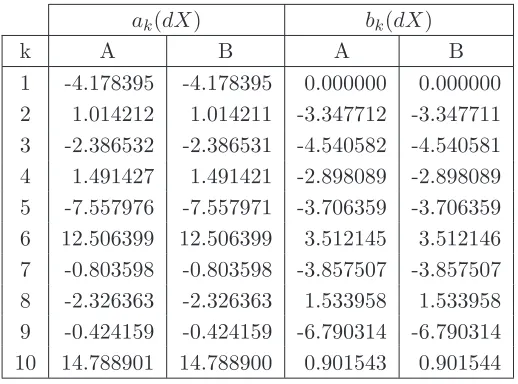
calculated by means of the FFT algorithm. To this purpose, we generate a series of prices using the diffusion model described in Chapter 1 with a sampling interval of 1 second for a total ofn= 7200 seconds. In order to mirror the market behavior and generate an irregularly traded series of prices, we randomly delete 20% of the transactions from the sample; the previous tick imputation scheme is then employed to interpolate the missing data and extend the length of the sequence to n = N + 1 = 8193, with N = 213. Finally, we calculate the Fourier coefficients using both the standard procedure and the one based on the FFT algorithm, we will hereafter refer to as theimproved procedure. In particular,

• we apply the standard procedure to the extended series of prices (scenario A);

• we apply the improved procedure to the extended series of prices (scenario B).

The output for the first 10 coefficients is summarized in the following table.

ak(dX) bk(dX)

k A B A B

[image:37.595.190.449.416.608.2]

1 -4.178395 -4.178395 0.000000 0.000000 2 1.014212 1.014211 -3.347712 -3.347711 3 -2.386532 -2.386531 -4.540582 -4.540581 4 1.491427 1.491421 -2.898089 -2.898089 5 -7.557976 -7.557971 -3.706359 -3.706359 6 12.506399 12.506399 3.512145 3.512146 7 -0.803598 -0.803598 -3.857507 -3.857507 8 -2.326363 -2.326363 1.533958 1.533958 9 -0.424159 -0.424159 -6.790314 -6.790314 10 14.788901 14.788900 0.901543 0.901544

Table 2.1: Fourier coefficients of price calculated with the standard procedure (column A) as opposed to the FFT algorithm (column B).

(38)

2.3. The optimal choice of the Fourier parameters 30

2.3 The optimal choice of the Fourier parameters

In applying the Fourier method to study ex post volatility dynamics, one is left with the problem of choosing the number of Fourier coefficients of priceN and the number of volatility coefficientsM to include in the estimation process, and to set the level of resolutionδ. Recall that the latter two quantities appear in the Fourier-F`ejer inversion formula

ˆ

σ_N,M2 (t) =a0(σ2) + M X

q=1

ϕ(δq)aq(σ2)cos(qt) +bq(σ2)sin(qt)

, (2.11)

where ϕ(δq) = sin₍_δq2(₎δq2), and with the volatility coefficients aq(σ2) and bq(σ2) as derived in

Theorem 1.1, Chapter 1, for the case i= j. If the process is observed at regular intervals, it is possible to define an upper limit for N. In particular, suppose that n observations are available; then N should not be set above the Nyquist critical level (see Priestley, 1979), in our case given by

fN yq =

1

2∆ (2.12)

where ∆ = T_n is the sampling interval, i.e. the time interval between consecutive samples. This is the fastest frequency that can be represented when data are recorded every ∆ units of time. IfN was set to a larger value, than the spectral density of the original process that lies outside the frequency range (₋fN yq, fN yq) would be aliased, i.e. falsely translated, into

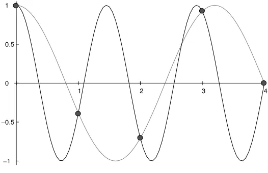
the range itself resulting in a corrupted reconstruction of the volatility trajectory. Before proceeding with the analysis, let us consider a simple example to illustrate the problem of aliasing from another prospective. Figure2.1 shows that a set of five data points (the dots) recorded every second can be delivered by sampling two sinusoids at different frequencies. In particular, it is clear that the cosine wave with the higher frequency (black line), which exceeds the Nyquist level, can be easily mistaken for the one with a lower frequency (gray line), since they are observationally indistinguishable. Also note that, by increasing the frequency even further, we would certainly find another sinusoid able to match the sample due to the periodicity of the trigonometric functions. Therefore, under the assumption of equally spaced data, we need to use enough Fourier coefficients of price to preserve the information on the original process, but we cannot exceed the maximum limit given in Eq. (2.12) either, otherwise the observed data will not adequately represent the price process itself, and so the underlying volatility dynamics.

(39)

−1 −0.5 0 0.5 1

[image:39.595.181.444.124.294.2]

1 2 3 4

Figure 2.1: Aliasing effect: the sinusoid with a frequency larger than the Nyquist (black line) and that one obtained with a lower frequency (gray line) are observationally indistinguishable. The dots represent the observed and equally spaced data points.

limit for the maximum frequency is no longer available. Intuitively, we can only expect N

to also exceed the Nyquist level when some points are located much closer than the average sampling rate, as it might be the case with irregularly spaced data. It is therefore important to know the maximum frequency content of the original process.

To deal with the problem of choosing an adeguate value forN but also for the frequencyM

and the smoothing parameterδ, we propose to employ a stochastic optimization algorithm to simultaneously estimate the three quantities. The algorithm is presented in the next section.

2.3.1 Joint optimization with Differential Evolution

The Differential Evolution (DE) algorithm belongs to the class of genetic or evolutionary methods that use mechanisms inspired by biological evolution, such as reproduction, mu-tation and natural selection, to solve difficult optimization problems. First introduced by Storn and Price(1997), DE is a population based method, in the sense that several solutions are considered at the same time to find the global minimum of a multidimensional, nonlin-ear and multimodal object function. Unlike other stochastic techniques that usually perturb existing results in accordance with a random quantity to locate new points on the search domain, DE uses weighted differences between decision space vectors to mutate elements of a current population and then generates new offspring’s.

In the Differential Evolution algorithm, individuals are represented byd-dimensional vectors of candidatesxi withi= 0,1, . . . , P −1, where dis the number of parameters and P is the

population size. For each solution xi of the current population, a new offspring solutionoi

(40)

oi where each element has a probability of π to come from oi and xi otherwise. The new

candidate solutionui therefore contains (combination of) values up to four current solutions:

xp1,xp2,xp3 andxi. If one element ofxhas the same value in all of these parenting solutions,

then so will the offspring; if they disagree, the offspring will either inherit xi’s values, with

a low probability of (1−π), or will be given a new value which is in the neighborhood of the corresponding value inxp1. Finally, if ui has lower objective value thanxi, the offspring

replacesxi, otherwise solution xi survives.

The fundamental steps of the algorithm are here summarized.

1. Initialization_{: select an upper and lower bound for each parameter}_d_{and collect these}

values into two d-dimensional vectorsbl and bu. Then, each element of the candidate

parametersxi is initialized by extracting a random value within this range as follows

xi,j =uj·(bj,u−bj,l) +bj,l j= 1, . . . , d

whereuj ∼U(0,1) is a uniformly distributed random number.

2. Mutation_{: recombine the population to obtain a vector of} _P _{trial values given by}

oi =xp1+F·(xp2 −xp3)

with i ₆= p1 6= p2 6= p3 ∈ [0, P −1] randomly sampled integers and F > 0 is a

real constant factor that determines the rate at which the populations evolves. This difference based mutation operator is the distinctive feature of the DE algorithm.

3. Crossover_{: construct a trial vector through a crossover operation which combines}

components from the current vector and from the mutant vector, according to a control parameterπ∈(0,1)

vi= (

oi ifU(0,1)< π

xi otherwise.

4. Selection_{: replace}_x_i _with_v_i _if_f₍_v_i₎_{< f}₍_x_i_{), for a given objective function}_f₍_x_).

Once the population is initialized, the process of mutation, crossover and selection is repeated through a finite number of generationsGuntil the optimum is located on the parameter space, or another termination criteria is satisfied, e.g. the maximum number of iterations Gmax is

(41)

2.4. Numerical analysis 33

Depending on the programming language in used, the implementation process of the the DE algorithm can be quite demanding as several technical details must be carefully considered. Moreover, to adapt the algorithm to the Fourier context an additional and substantial effort is required. To partially assist our work, we have referred to the book byPrice et al. (2005), which offers an extended description of the method with a comprehensive overview of the aforementioned details (see Chapter 2 therein), including useful pseudo-code and sample applications. See also Maringer and Meyer (2008) for an accurate comparison of different evolutionary algorithms and the most recent developments in the field.

2.4 Numerical analysis

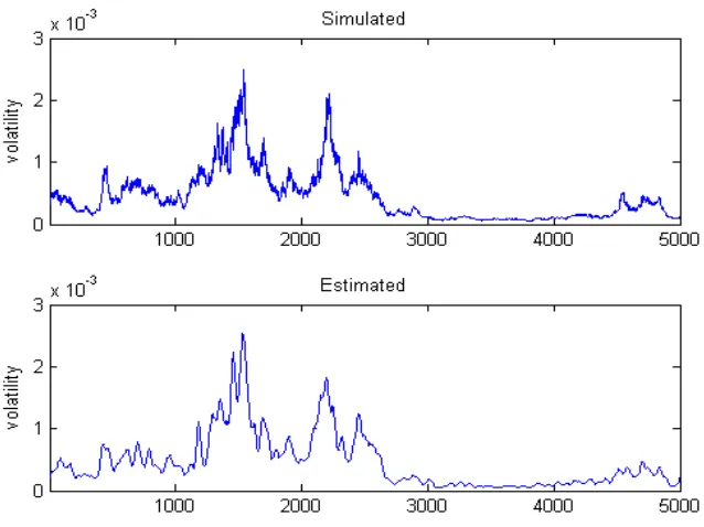
We will start with a simple example of spot volatility estimation in order to understand how the Fourier method works. A detailed analysis of the estimation process will be developed in the second part of the section. Consider the short interest rate model introduced by Chan et al. (1992). This is a broad class of processes that includes the mean reverting version of the Ornstein-Uhlenbeck process proposed by Vasicek (1977) and the one-factor general equilibrium model developed inCox et al.(1985). It is defined as the solution of the following stochastic differential equation

d r(t) =β(α₋r(t))dt+ηrγ(t)dW(t). (2.13) To simulate the process, we have used the parameters estimated in Jiang (1998) on the 3-month Treasury bill rates via an indirect inference approach and given by ˆα= 0.079,

ˆ

β= 0.093, ˆγ = 1.474, and ˆη = 0.794. Figure 2.2 illustrates the temporal behavior of the diffusion coefficient σ2₍_t_{) = ˆ}_η2_r2ˆγ₍_t_{) on 5}_,_{000 daily prices obtained by sampling the process}

r(t). The estimate obtained with the Fourier methodology is showed to well follow the dy-namics of the simulated path, leading to a good pointwise reconstruction of the volatility trajectory. In particular, it is important to point out that the latter was obtained directly from the generated interest rates values and not from the simulated diffusion process, here used only for comparison.

2.4.1 Simulation design