Comparison of Analytic Inversion Techniques for Equalisation of Highly Frequency Selective MIMO Systems

COMPARISON OF ANALYTIC INVERSION TECHNIQUES FOR

EQUALISATION OF HIGHLY FREQUENCY-SELECTIVE MIMO SYSTEMS

Viktor Bale and Stephan Weiss

Communications Research Group

School of Electronics & Computer Science

University of Southampton UK, SO17 1BJ

E-mail:

{

vb01r,sw1

}

@ecs.soton.ac.uk

ABSTRACT

This paper discusses MIMO equalisers created by analytic inversion of a known frequency-selective MIMO channel. It considers inversion performed in thez-domain, time-domain using convolutional matrices, and the frequency-domain. It explains the criteria of these inversions and compares the per-formances in terms of MSE between the input and output to a concatenated channel-equaliser system through use of sim-ulations, and puts these results into context in terms of com-putational cost.

1. INTRODUCTION

In recent years, theoretical and practical investigations have shown that it is possible to realise enormous channel ca-pacities, far in excess of the point-to-point capacity given by the Shannon-Hartley law [1]. The majority of work to date on this area has assumed flat sub-channels composing the multiple-input multiple-output (MIMO) channel. As the aim of MIMO systems is often to increase the data transmis-sion rate of a communication system, a wideband and hence highly time-dispersive model would seem more appropriate. To properly exploit this environment to realise these capac-ity increases, the MIMO channel must be equalised for both the cross-channel interference (CCI) between MIMO sub-channels and the inter-symbol interference (ISI) inherent to broadband channels, so that the performance of any system attempting to harness the multipath diversity can do so while maintaining a satisfactory bit error rate (BER) performance. Creating a system that performs equalisation with a satisfac-tory performance for a highly time-dispersive MIMO system is far from a simple task.

Generally, creating an equaliser will require inverting the system. One such technique is by adaptive inversion of the MIMO system [2]. While this technique results in a satisfac-tory MIMO equaliser for recovering signals passed through extremely hostile highly frequency-selective systems, the adaptation is still slow, requiring tens of thousands of nor-malised least mean squared (NLMS) algorithm iterations be-fore the adaptive systems converges to an acceptably low mean squared error (MSE). If the channel has a sufficiently high coherence time then this will not cause any problems, however for fast moving mobile stations (MS) it is desirable

to have a system that can find an equaliser as quickly as pos-sible. Secondly, the adaptive inversion can consume a large amount of computational power, which may be at a premium in a MS, so again we are motivated to create a system which can quickly invert the MIMO system to create an equaliser, and to keep the complexity of this system as low as possible. It is well-known that adaptive algorithms such as NLMS can converge quickly to short channels and where the input signal to the algorithm is spectrally flat. An adaptive FIR system to identify an unknown MIMO channel is generally shorter than the system to invert it, and also in the identifica-tion set-up the input signal can be chosen to be white. This is not the case for the adaptive inversion set-up where the algorithm input is coloured by the frequency-selective chan-nel. Hence, we propose that we can adaptively identify the unknown MIMO system, and then analytically invert it at the receiver. In this paper, we will assume the MIMO channel is known from a previous identification, and we look at tech-niques to analytically invert it.

Section 2 outlines the system model used in this paper. Section 3 shows an zero-forcing (ZF) MIMO inversion and stabilisation technique which give an IIR equaliser, while Section 4 shows a time-domain method for finding a MMSE FIR MIMO equaliser. Section 5 outlines a frequency-domain method for finding a FIR MIMO equaliser, which although sub-optimal can be calculated at a significantly lower com-putational cost that the other methods, and shows how to combat circular convolution effect inherent to this method. Section 6 shows simulation performance results for the three methods applied to three MIMO channels with differing characteristics, and Section 7 draws conclusions.

2. SYSTEM MODEL

In the following section we will be calculating the channel inverse in three different domains, and therefore the problem must be also formulated in these domains. We now express the system model in a domain-independent representation, so that we can use this as a base to convert to the required domain in the following sections.

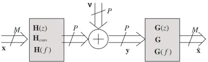
The output of the MIMO channel is given by

Hconv

H(z)

H( f )

G G(z)

G( f )

M P P M

P

x _y

νννν

xˆ

Fig. 1. Schematic of a known MIMO channel and a MIMO equaliser shown in three different domains.

whereyis a vector of output signals from the known MIMO channel,H, corrupted by AWGNν, andxis a vector of the

input signals. The structures of these variables are undefined at this point as they depend on the representation domain. Figure 1 shows this system in combination with a suitable MIMO equaliserG.

3. Z-DOMAIN INVERSION

A simple method to calculate the inverse of a MIMO system is to express the problem in thez-domain and algebraically invert the MIMO matrix. In general, this will result in an IIR system, and although the method is very simple and can lead to an excellent solution in some cases, it can also lead to an unstable solution. Whilst we can use a technique to stabilise the unstable parts of the IIR system, other problems arise if the problem is ill-conditioned that cannot be easily solved.

We start by expressing the MIMO system matrix in the z-domain

H(z) =



 

h11(z) · · · hM1(z) ..

. ...

h1P(z) · · · hM P(z)





, (2)

wherehmp(z) =hmp(0)z0+hmp(1)z−1+· · ·+

hmp(Lh+1)z−Lh+1andLhis the length of the MIMO

chan-nel impulse response. Hence the system function becomes

y(z) = H(z)x(z) +ν(z), and the elements of the vectors

and matrix are all functions inz. The inverse criterion can now be expressed

G(z)H(z) =z−dI, (3)

which results in the zero-forcing solution. The inverseG(z)

is given by

G(z) = (zdH˜(z)H(z))−1_˜

H(z), (4)

whereH˜ is the parahermitian onH[3].

The inversion ofH˜(z)H(z)can be found using the stan-dard Gaussian algebraic elimination method, where we per-form row operations on the polynomials in z in the same way as if they where scalars. The inverse is stable if

det( ˜H(z)H(z))is minimum phase. Problems arise when the determinant is non-minimum phase and therefore we must use a stabilisation technique where we express the determi-nant polynomial in terms of its roots. The roots with a mag-nitude less than one can be reconstructed into a stable IIR

system. The remaining roots are expressed in partial fraction form and then converted into stable infinite length anti-causal FIR systems using the relationship

1 1−az =

∞

X

n=0

anzn |a|<1, (5)

whereais the reciprocal of the pole, and taking care to deal with multiple co-located poles correctly. We now truncate this at an appropriate value fornwhereanhas decayed to a suitably small value, and introduce a delay to make the sys-tem causal. This forms the basis for a delayed causal stable FIR approximation of an unstable IIR system.

While this works well in theory, in practice an ill-conditioned MIMO system where the determinants have roots near the unit circle in thez-domain can cause fatal prob-lems. During the stabilisation process we need to calculate the roots of the determinant polynomial, but this operation is very prone to finite accuracy round-off errors during com-putation. After the stabilisation operations on the roots the polynomial must be reconstructed and the small inaccuracies in the root-finding operation are magnified so that previously stable parts of the determinant close to but inside the unit circle have now migrated to outside the unit circle and have become unstable. The only obvious solution to this is to in-crease the machine accuracy so that the roots can be accu-rately found.

If the determinant can be guaranteed to be minimum phase we can cut out the stabilisation process and thisz-domain method not only works very well, but has a low computa-tional complexity ofO(Lhlog2Lh)for a MIMO system of

fixed dimensions, assuming the convolutions in the calcula-tion ofH˜(z)H(z)in the determinant are performed using FFTs. If the determinant is non-minimum phase and there are no determinant roots near the unit circle good performance is still possible using the stabilisation process, although the computational complexity becomesO(L3

h).

In a low noise environment where the determinant of the channel has no roots near the unit circle, thisz-domain tech-nique can work very well and quickly. Unfortunately, we cannot usually guarantee that the determinant will either be minimum phase, or have no roots near the unit circle when it is non-minimum phase, and so this method is unsuitable for the equalisation of MIMO systems in general. Also, the ZF solution will generally not exhibit favourable behaviour in a noisy environment, and the calculation of an MMSE solution in thez-domain is very complicated [4].

4. TIME-DOMAIN INVERSION

be-tween transmittermand receiverpis given by

Hmp=



    

hH

mp · · · 0 0

0 hH

mp · · · . .. 0

0 0 . .. . .. ...

0 0 · · · hHmp · · ·



    

, (6)

where hmp = [hmp[0] · · · hmp[Lh −1]]H is the

sub-channel impulse response. We may construct a parent con-volutional matrixHover allmandp, yielding

Hconv=



   

H11 H21 · · · HM1

H12 H22 · · · HM2 ..

. ... . .. ...

H1P H2P · · · HM P



   

, (7)

whereHconvis of dimensionsP Lg×M(Lh+Lg−1)and

Lg is the chosen length of the MISO equaliser filters.

Us-ing this we create a transmission modely = Hconvx+ν,

wherexis a lengthM(Lh+Lg−1)stacked vector

repre-senting the input to the MIMO system, _ν is a lengthP Lg

vector representing AWGN and y is a length P Lg vector

representing the output. Note that both the varying nature of the signals in time and the multiple inputs/output are rep-resented in one dimension in the input, output and noise vec-tors. To find the MIMO equaliser we must obtain a ma-trix G so that after a signal is passed through the chan-nel and equaliser, there should ideally only be a delay. We may findGusing the well-known Weiner-Hopf solution [7],

gm = R−1pm where gm = [gHm1 g

H

m2 · · · g

H mP]

H

and gmp = [gmp[0] gmp[1] · · · gmp[Lg −1]]H.

Af-ter some mathematical development we can calculate that

R=σ2

xHconvHHconv+σ 2

νI, assuming that all the input

vari-ances and noise powers are the same, whereσ2

xis the power

of the input signalx[n]andσ2

νis the power of the noiseν[n]

at each receiver. Also, we can shown thatpm =Hconvdm, wheredmis a channel selection and delay vector. We may now findgm = (σ2

xHconvHHconv+σ 2

νI)†Hconvdm, where we have used the pseudo-inverse{·}†_{for valid cases where} M > P andHconvHHconvmay be rank-deficient. After fur-ther mathematical development we can relate this to the reg-ularised pseudo-inverse of the channel

gH_m = dH_m¡

HH_convHconv+HHconvRν(H

H

conv)†

¢−1

HH_conv(8)

= dH_m¡

HH_convHconv+σν2I

¢−1

HH_conv, (9)

where Rν is the auto-correlation matrix of the noise. We

must, of course, perform this calculationM times for each of the transmitted data streams and can then stack thegm’s

to create the MIMO equaliser matrix G. The main differ-ence between this method and the z-domain method in the previous section is that this will always produce a FIR solu-tion while the z-domain method will in general produce an IIR solution. Also, with this method we are free to choose the length of the equaliser so we can always choose it to give good performance, albeit that this will be at the expense of

greater computational complexity for the equaliser calcula-tion.

While the method usually works well, the complexity can become large very quickly with an increasing Lg, due to

the fact that this causes both dimensions of Hconv to in-crease. After some algebraic development the complexity with respect toLg involved in calculatinggm∀m ∈ 1 :M

can be shown to beO(L3

g). Notice that this is greater than

theO(L3

h)of thez-domain method, as generally we choose

Lg > Lh. From this we see that it is beneficial for

compu-tational simplicity to keepLg as low as possible while still

achieving satisfactory performance. Alternatively we may seek a lower complexity method.

5. FREQUENCY-DOMAIN INVERSION

We may arrange for the impulse responses of the sub-channels to be transformed into their spectral representa-tions, and hence formulate the problem in the frequency do-main. In this case the elements of the MIMO channel matrix are functions of frequency, as are the elements ofx,ν and

y. Hence we have the frequency-domain system function

y(f) =H(f)x(f)+ν(f). We may use the FFT to obtain the

frequency-domain representations of the time-domain sig-nals. The main advantage of processing the problem in the frequency-domain is that the inversion ofH becomes very simple as we may now deal withKscalar valued MIMO ma-trices for each frequency bin which are independent, where K in the number of frequency bins of the FFT, and invert each matrix using the standard algebraic method. We use the pseudo-inverse

GH[f] =e−j2πf d¡

HH[f]H[f]¢−1

HH[f], (10)

wheree−j2πf d_{is adsymbol delay in the columns to make}

the non-causal part of the response realisable. After we have calculatedG[f]we simply applyKIFFTs across each ele-ment of all the scalar-valued spectral inverse matrices. Per-forming adaptation in the frequency-domain, however, pro-vides its own challenges, as for example the system must wait to accumulate enough data on which so perform the FFT. Another problem not present with the time-domain method is that of circular convolution effects caused by performing frequency-domain processing [8]. The usual method to over-come this is by zero-padding the channel to at least length

2Lh. Fortunately this is implicit to be method as we choose

a lengthLgFFT to obtain an equaliser of the correct length

and we usually chooseLg>2Lh, hence we avoid this

this frequency-domain method, due to the wrap-around ef-fects. However, at low SNRs where the error due to noise dominates over the error due to the wrap-around effects it is still be beneficial to regularise by the noise power. In these cases the performance is the same as the optimum MMSE time-domain solution. The regularised solution is given by

GH[f] =e−j2πf d¡

HH[f]H[f] +βI¢−1

HH[f]. (11)

At low SNRs we may choose β = σ2

ν as with the

time-domain method, and then at some critical SNR switch to a fixed value forβthat regularises for the wrap-around effects. The complexity of this frequency-domain method is domi-nated by the FFTs that are required during its execution, and so isO(Lglog2Lg), which is by far the lowest of the three

methods.

6. SIMULATIONS

For the simulations we use three MIMO channels. The first is a2×2channel with length 2 FIR sub-channels, and the eigenvalue spread of the convolutional MIMO channel ma-trix, H, which gives a measure of the difficulty in inverting the MIMO channel using the time-domain technique in Sec-tion 4 is about 20 [7]. The MIMO channel determinant is non-minimum phase and hence the IIR inverse is unstable, but there are no zeros near the unit circle. The second and third channels are2×2MIMO channels based on measure-ments taken from the Signal Processing Information Base (SPIB) at Rice University [10] and in both cases the sub-channel comprising the MIMO sub-channel are truncated to 50 taps and start from just before the main part of the response. The second MIMO channel uses the unmodified channels from SPIB, and the MIMO channel has a minimum phase determinant in thez-domain. The RMS delay spread of the sub-channels are between6.6ns and0.4µs, and the eigen-value spread of the convolutional MIMO channel is 13. For the third MIMO channel, the channels are modified to make them very frequency-selective, creating an extremely hostile

2×2MIMO system with a non-minimum phase determinant with poles near the unit circle in thez-domain. In this case the RMS delay spread is between0.4µsand0.5µsand the eigenvalue spread of the convolutional MIMO channel ma-trix is 962. Thez-domain inversion is ZF, the time-domain inversion is MMSE and the frequency-domain inversion is a regularised ZF that approaches the MMSE at low SNRs. The MSE is assessed by passing white noise through the con-catenated channel-equaliser system, and measuring the dif-ference between the input and output.

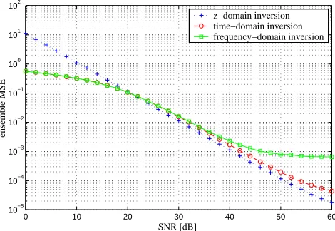
Figure 2 shows the three equalisers calculated from inver-sion in the relevant domains using the first channel. The z-domain inversion is possible as there are no poles near the unit circle so we employ the stabilisation technique de-scribed in Section 3 using a length 32 FIR filter to approxi-mate the unstable part of the IIR determinant. With both the time-domain and frequency-domain inversion we also use a length 32 FIR inverse. We see that at low SNRs the time-domain and frequency-time-domain techniques perform similarly

0 10 20 30 40 50 60

10−5 10−4 10−3 10−2 10−1 100 101 102

SNR [dB]

ensemble MSE

z−domain inversion time−domain inversion frequency−domain inversion

Fig. 2. MSE curves forz, time and frequency-domain inver-sion in a mildly time-dispersive noisy environment.

and both are much better than thez-domain technique of ac-count of the different inversion criterion. At mid SNR levels all the performances are similar but at high SNRs we see that the z-domain technique is superior due to its IIR part; re-member that thez-domain inverse still retains this from the stable part of the IIR determinant. The time-domain method follows closely, with the frequency-domain technique per-forming somewhat worse. In Section 5 we explained that we should use a regularisation factor even in a noiseless envi-ronment on account of the circular convolution effects but here the optimum factor is found to be approximately zero, so this is the best performance possible with the frequency-domain technique. The frequency-frequency-domain method appears to result in the best performance compromise in terms of MSE, which is the same as optimum MMSE performance at the more realistic lower SNR values, and at a considerably lower computational cost that the time-domain method.

Figure 3 shows the performance of inversion with the severely time-dispersive MIMO channel with a minimum phase determinant. We use length 280 filters for the time-domain and frequency-time-domain equalisers. At low and mid SNR the results are similar to the mildly time-dispersive channel. At high SNR thez-domain method is still the best, but the time-domain and frequency-domain inverse perfor-mances are much closer to each other now. As the determi-nant is minimum phase no stabilisation is required for thez -domain inversion, and so this method has significantly lower computational complexity than the other two methods. Also its performance is only 3 dB worse that the MMSE case at SNR=0, which may be deemed acceptable given the compu-tation savings.

0 10 20 30 40 50 60 10−6

10−5 10−4 10−3 10−2 10−1 100 101

SNR [dB]

ensemble MSE

z−domain inversion time−domain inversion frequency−domain inversion

Fig. 3. MSE curves forz, time and frequency-domain inver-sion in a severely time-dispersive noisy environment with a minimum phase channel determinant.

0 10 20 30 40 50 60

10−3 10−2 10−1 100 101 102

SNR [dB]

ensemble MSE

time−domain

frequency−domain regularised by noise power

frequency−domain regularised by noiseless optimum (0.0001)

Fig. 4. MSE curves forz, time and frequency-domain inver-sion in a severely time-dispersive noisy environment with a non-minimum phase channel determinant.

high SNR the noise power drops below the optimum noise-less regularisation factor found to be approximately 0.0001, hence the MSE rises again. We also show a curve were the inverse is regularised by this noiseless optimum across all SNRs. Hence we could use the frequency-domain method at all SNRs but switching the regularisation factor at about 30 dB SNR. Once again the time-domain methods results in the optimum MMSE solution but at significant computational cost. We could argue that the computational overhead does not warrant the improvement in MSE at high SNRs where the frequency-domain method regularised by the noiseless optimum value performs satisfactorily, depending on the re-quired performance for the application. Finally, notice that in all simulations the performance of the frequency-domain method regularised by noise power approaches that of the MMSE time-domain method at low SNRs, as the observation noise dominates over the effects of the circular convolution.

7. CONCLUSIONS

We have considered the MSE performance and stated the computational complexity order of three different kinds of analytic inversion techniques for frequency-selective MIMO channels. We outlined the limitations and benefits of each of these techniques and showed when they could or could not be used. We saw that for mildly time-dispersive channels the frequency-domain inversion gave the best performance promise across the more realistic lower SNR range at a com-putational cost significantly lower than that of the MMSE time-domain method. For severely time-dispersive MIMO channels with a minimum phase determinant, thez-domain inversion gave the best performance compromise in terms of MSE and the lowest computational cost since no stabilisation was required. With severely time-dispersive MIMO channels with a non-minimum phase determinant and poles near the unit circle, thez-domain method cannot be used. Although the time-domain method gave the best MSE performance compromise across the whole range, the frequency-domain technique also gave a satisfactory performance by switching the regularisation factor when the noise power falls below the optimum noiseless factor, at a much reduced computational cost.

8. REFERENCES

[1] G. J. Foschini and M. J. Gans, “On limits of wireless commu-nications in a fading environment when using multiple anten-nas,” Wireless Personal Communcations, , no. 6, pp. 315–335, 1998.

[2] V. Bale, Mini-thesis: Multiple-Input Multiple-Out-put Sys-tems: Fullband and Subband Adaptive Techniques, University of Southampton, UK, 2004.

[3] P. P. Vaidyanathan, Multirate Systems and Filter Banks, Pren-tice Hall, Englewood Cliffs, 1993.

[4] A. Ahl´en and M. Sternad, “Wiener Filter Design Using Poly-nomial Equations,” IEEE Transactions on Signal Processing, vol. 39, no. 11, pp. 2387–2399, November 1991.

[5] O. Kirkeby, P. A. Nelson, F. Orduna-Bustamante, and H. Hamada, “Local sound field reproduction using digital sig-nal processing,” Joursig-nal of the Acoustical Society of America, vol. Vol.100, no. No.3, pp. 1584–1593, March 1996. [6] V. Bale and S. Weiss, “An Optimum Linear

Frequency-Selective MIMO Equaliser using Time-Domain Analytic In-version,” in PREP Postgraduate Research Conference, Uni-versity of Hertfordshire, UK, April 2004, vol. Oral Presenta-tions, pp. 24–25.

[7] S. Haykin, Adaptive Filter Theory, Prentice Hall, Englewood Cliffs, 3rd edition, 1996.

[8] J. J. Shynk, “Frequency-Domain and Multirate Adaptive Fil-tering,” IEEE Signal Processing Magazine, vol. 9, no. 1, pp. 14–37, January 1992.

[9] O. Kirkeby, P. A. Nelson, H. Hamada, and F. Orduna-Bustamante, “Fast Deconvolution of Multichannel Systems Using Regularization,” IEEE Transactions on Speech and Au-dio Processing, vol. 6, no. 2, pp. 189–194, March 1998. [10] “Signal Processing Information Base: Micro-wave Channel