Exploring Deep Neural Network Models for Classification of High-resolution Panoramas

(1)

Rochester Institute of Technology

RIT Scholar Works

Theses

5-2019

Exploring Deep Neural Network Models for

Classification of High-resolution Panoramas

(2)

Exploring Deep Neural Network Models for Classification of

High-resolution Panoramas

APPROVED BY

SUPERVISING COMMITTEE:

Dr. Christopher Kanan, Supervisor

Dr. Thomas Kinsman, Reader

(3)

Exploring Deep Neural Network Models for Classification of

by

Deepak Sharma

THESIS

Presented to the Faculty of the Department of Computer Science

Golisano College of Computer and Information Sciences

Rochester Institute of Technology

in Partial Fulfillment

of the Requirements

for the Degree of

Master of Science

(4)

Abstract

Exploring Deep Neural Network Models for Classification of

Deepak Sharma, M.S.

Rochester Institute of Technology, 2019

Supervisor: Dr. Christopher Kanan

The objective of this thesis is to explore Deep Learning algorithms for classifying high-resolution

images. While most deep learning algorithms focus on relatively low-resolution imagery (under

400×400pixels), very high-resolution image classification poses unique challenges. These

im-ages occur in pathology and remote sensing, but here we focus on the classification of invasive

plant species. We aimed to develop a computer vision system that can provide geo-coordinates

of the locations of invasive plants by processing Google Map Street View images at using finite

computational resources. We explore six methods for classifying these images and compare them.

Our results could significantly impact the management of invasive plant species, which pose both

(5)

Acknowledgments

I wish to thank the multitudes of people who helped and supported me to complete the

thesis. Time would fail me to tell of my advisor, Dr. Christopher Kanan for providing me constant

guidance during the thesis coursework and providing me with access to all resource while working

on the problem. He also provided me with a lifetime cherishable opportunity for interacting with

leading researchers in the field of Deep Learning for discussing this problem and exploring solution

with them. I also would like to thank Dr. Thomas Kinsman for providing his valuable advice while

exploring various techniques. Your door was always open for me whenever I had questions related

to fundamental topics of Computer Vision and Data Science. I would like to use this opportunity to

express my gratitude to Dr. Zack Butler for his insightful support and for the immense knowledge

that guided me to conduct this thesis which helped me to prepare for the necessary deliverables.

Sincere thanks to Arturo Flores, Meg Wilkinson, Dr. Kaitlin Stack Whitney for providing the

Dataset.

Besides my thesis committee, I would like to thank Dr. Hans-Peter Bischof for allowing me

to explore the problem under the thesis program and strengthen my research capabilities. I deeply

appreciate the help and support of my academic advisor Cindy Wolfer at every phase of graduate

life. I greatly value the friendship of Preeti Sah and Avinav Sharan for their support and grateful

to them for reviewing my report. Finally, I would like to express my very profound gratitude to

my parents and sisters for providing me with unfailing support and continuous encouragement

(6)

List of Tables

3.1 Count of the labeled samples . . . 19

4.1 Results for Cluttered MNIST dataset . . . 45 4.2 Comparison among various methods for classifying invasive plants. All ResNet18

models are pre-trained with ImageNet dataset accept other vise mentioned. . . 55

(10)

List of Figures

1.1 A sample Google Street View image showing invasive plants . . . 2 1.2 Non-Native Phragmities affected states of the USA(image reproduced from [1]

using mapping tool [2]) . . . 3 1.3 Non-Native Phragmities affected counties of The New-York state(image

repro-duced from [1] using mapping tool [2]) . . . 4 1.4 Japanees Knowtweed affected states of the USA(image reproduced from [3] using

mapping tool [2]) . . . 6 1.5 Japanese Knotweed affected counties of the New-York state(image reproduced

from [3] using mapping tool [2]) . . . 8 1.6 Changing appearance of the Non-Native Phragmites and Japanese Knotweed

dur-ing different seasons . . . 10

3.1 Spatial Distribution of the detect areas containing invasive plants. . . 20 3.2 Cropped image after identifying regions affected by invasive plants which

signifi-cantly reduces image size. . . 20 3.3 Example sub-image of size224×224for the background class. . . 23 3.4 Example sub-image of size224×224for the invasive class. . . 23 3.5 Dynamic Capacity Network for classifying Cluttered MNIST dataset. Size of

out-put feature map for each layer is shown adjacent to each layer box. . . 26 3.6 DCN network for classifying Google Street View images. Fine sub-network

con-tains more layers than Coarse sub-network. Both sub-network have equal receptive fields. . . 31 3.7 An invasive plant image generated by inserting cropped part containing invasive

plant in a non-invasive plant image. . . 34

4.1 ROC and PR curves for the finetune ResNet18 model with test images of size 224×224 . . . 38 4.2 ROC and PR curves for the finetune ResNet18 model with test images of size

1400×6156 . . . 39 4.3 ROC and PR curves for the finetune modified ResNet18 model with test images of

(11)

4.4 ROC and PR curves for the finetune ResNet18 model with test sub-images of size 224×224 . . . 41 4.5 ROC and PR curves for the finetune ResNet18 model with all sub-images of size

224×224 . . . 42 4.6 ROC and PR curves for the algorithm 1 . . . 43 4.7 Showing14bounding boxes of the size18×18corresponding the spatial parts of

images selected for passing through the Fine sub-network. . . 46 4.8 ROC and PR curve for the finetune ResNet18 model with test sub-images of size

700×3328. . . 49 4.9 ROC and PR curve for the finetune ResNet18 model with test sub-images of size

2800×832. . . 50 4.11 Showing25bounding boxes of the size224×224corresponding the spatial parts

of images selected as input for the Fine sub-network. . . 52 4.13 Showing 25 bounding boxes of the size224×224corresponding the spatial parts

of images selected as input for the Fine sub-network. . . 54

(12)

Chapter 1

Introduction

1.1

Objective

The objective of this thesis is to develop a generic applicable computer vision

methodol-ogy for classifying high-resolution images. Such methodolmethodol-ogy is applicable in various aspects of

human life. Existing instances of such classifiers are in the field of pathology to develop an

ef-fective system for classifying cancer images [7] or brain tumor analysis [8] and also in the field

of satellite image analysis. While developing a high-resolution image classification, we have also

tried to solve a real-world problem of identifying locations in the USA affected by invasive plants.

We aimed to develop a computer vision system which can provide geo-coordinates of the locations

of invasive plants by processing Google Street View images at large scale using finite computation

resources and time. Our algorithm is also generic and it can be easily reconfigured for detecting

other invasive plants and solving other problems related to the classification of high-resolution

images.

1.2

Invasive Plant Classification System

Currently, we are aiming to detect two invasive species for grass: Non-native Phragmites

andJapanese Knotweed. At later stages, our generic method can be applied to other invasive plants

(13)

Environmental protection organizations like New York Department of Environmental

Con-servation can use our system for identifying affected areas for precisely marking Geo-locations of

these invasive plants. Using Google Street View API[9] all the Google Street View images for a

ge-ographic region can be downloaded, then our system will identify the images where invasive plants

are present. Finally, using geo-coordinates associated with images containing invasive plants, the

precise geo-location of the plants can be reported. A sample Google Street View image is shown

in figure 1.1 In general, for a geographical area, the number of images not containing any invasive

plants will be larger than the number of images containing invasive plants. Thus we aim to develop

an image classification system with a low number of false negatives.

There are many methodologies available for removing invasive plants, however, the New

[image:13.612.73.545.343.583.2]

York Department of Environmental Conservation is facing challenges in locating these plants.

(14)

[image:14.612.90.513.153.423.2]

1.2.1 Invasive Plants and Their Impact on Biodiversity 1.2.1.1 Non-native Phragmites

(15)

[image:15.612.77.527.82.429.2]

Figure 1.3: Non-Native Phragmities affected counties of The New-York state(image reproduced from [1] using mapping tool [2])

During the era of the industrial revolution in the 18th and 19th centuries, ancestors of

the non-native phragmites reached the eastern shores of the USA. Today, non-native Phragmites

are spreading throughout the continental states as shown in Figure 1.2. Eastern coastal states

are the most affected areas. Figure 1.3 shows New York state is severely affected by invasive

plants. In many parts of these affected regions, native marshland and wetland flora have been

(16)

are firmly impacted due to the fast growth of the perennial Non-native Phragmites. Non-native

Phragmites form dense monotypic culture which consumes all available nearby space, as a result,

other native plants get displaced [10, 11, 12]. Marks has found that Non-native Phragmites is

the most important factor for the exclusion of other brackish tidal marsh species [13]. In Adolph

Rotundo Wildlife Preserve in Massachusetts, the population of seeds of triangle orache and seaside

goldenrod species has decreased significantly. It has been found that, due to such encroachment

by non-native Phragmites, fauna dwelling in these areas lost their habitats. In brackish marshes of

Connecticut’s tidal wetlands, there was a significantly fewer presence of endangered bird species

in the area hogged by non-native Phragmites than the area occupied by saltmeadow rush, saltgrass,

and/or cordgrass. On the Hog Islands of southern New Jersey, the fish population has significantly

reduced in the regions affected by non-native Phragmites. They can also alter the hydrology of

wetlands by changing the flow of water and by replacing previous dominant vegetation, they can

alter soil properties, salinity levels, and topographic relief. For example, at Hog Island in southern

New Jersey, water salinity, depth to water table, and topographic relief were significantly lower in

areas dominated by Non-native Phragmites than area dominated by salt-meadow cord-grass and

salt-grass. Also, Non-native Phragmites can increase the chances of wildfire [13].

1.2.1.2 Japanese Knotweed

Unlike non-native Phragmites, Japanese Knotweed was intentionally introduced to the US

from Japan, China, and Korea around 1800. But in 1930 it was identified as an invasive plant.

Like non-native Phragmites, Japanese Knotweed also develops mono-culture by replacing native

flora. It is a perennial robust plant which can grow rapidly round disturbed area, old homes along

(17)

[image:17.612.94.525.199.459.2]

(18)

are affected by this plant, Japanese Knotweed displaces streamside vegetation by limiting sunlight

or nutrients as shown on the map 1.4. Claeson et al. have found leaf litter from native species

was reduced significantly in Japanese Knotweed invaded riparian areas of Washington State [14].

In addition, they can suppress the growth of other native plants by releasing toxic or inhibiting

chemicals. Hence Japanese Knotweed severely affects host ecosystems by out-competing native

vegetation and limiting species diversity, which reduces species diversity for both flora and fauna.

Dense stands of Japanese Knotweed clog waterways and expedite erosion and harming riparian

habitat for fish and other animals. Japanese Knotweed intercepts rainwater by densely shedding

the small streams. It can also result in blocking flood infrastructure such as drains and ditches

(19)

[image:19.612.83.534.154.506.2]

(20)

1.2.2 Challenges

Even though these invasive plants are present in abundance locating these plants is a major

problem due to reasons like change in the appearance during different seasons, varying luminosity

amount, plants were out of camera focus, and distance of the plant from the camera.

1.2.2.1 Changing appearance of the invasive plants

A major challenge for the proposed classification model is not only to differentiate

Non-native Phragmites and Japanese Knotweed from other similar looking species of grass but also to

take into account the fact that the look and shape of these plants vary during the different seasons

of the year. For example, Non-native Phragmites becomes golden and purple from green in the

month of August. This changing appearances of invasive plants during the year makes the task of

their detection difficult. In such scenarios, we are unable to come up with an early rejection system

where just by analyzing color information of the image, we can discard areas of images for any

(21)

(a) Non-Native Phragmites during Fall(image repro-duced from [18])

(b) Non-Native Phragmites during summer(image re-produced from [? ])

(c) Japanese Knotweed during summer(image repro-duced from [19])

[image:21.612.76.539.155.308.2]

(d) Japanese Knotweed during spring(image repro-duced from [20])

(22)

1.2.2.2 Varying luminosity

Since the Google Street View images are taken during the various time of the day, the

sunlight varies for the camera which results in the variation in intensity level of the images. Image

of the same object taking with varying luminosity produce variation in color composition. Such

variation offers a challenge for any image classification algorithm.

1.2.2.3 Unfocused object of interest

Google Street View images are taken from a wide-angle camera, which is designed for

capturing large areas. These images are taken from a moving vehicle and the camera does not

focus on any particular object. Since the object of our interest – invasive plant – is not necessarily

in focus, the resultant images have less descriptive feature associated with the invasive plants. Also

because the descriptiveness of feature is associated with the uniqueness of an object or part of the

object, the inter-class variation will be reduced between two similar looking objects. As a result,

classification algorithms like SVM [21] or Deep Learning based neural network may not identify

the object of interest with high confidence.

1.2.2.4 Distance of plants from the camera

Since the plants can be at any arbitrary distance from the camera, the texture associated

with the same spices plants will differ and also the resolution of plants which are at a far distance

from the camera will also be reduced. Due to these factor identification of invasive plants will be

(23)

Chapter 2

Image Classification

Object recognition is a fundamental problem in Computer Vision. A series of

methodolo-gies have surfaced in the last two decades for solving this.

2.1

Image classification

To perform image classification, earlier shallow learning approaches represented an image

as an order-less collection of local features. Such representation was referred to as the ’bag of

features’. Subsequently, these global feature representations were classified using classifiers such

as SVM [21].

A plethora of methods for extracting local features was proposed during the same time

frame. Feature extraction methods such as Scale-Invariant Feature Transform (SIFT) [22],

His-togram of Oriented Gradients(HOG) [23], Local Binary Pattern(LBP) [24] and their variants [25]

have been used across object recognition algorithms. The accuracy of a classification model

de-pended on the relevancy of the feature representation. Typically, synthesizing a relevant feature

extraction method was a tedious task and required domain knowledge. In a number of object

recognition solutions, an encoding algorithm was used for reducing the dimensionality of the local

feature vectors. Finally, the global feature vector for the image was produced by either using some

(24)

(FV) [26].

In the last decade, researchers were trying to develop generic methodologies for classifying

any given object because generic processes are more effective as they are applicable to a whole

spectrum of object classification problems. To achieve such a generic process, many complex

solutions had emerged. Like Yu et al. used an encoding algorithm for reducing the dimension

of these features along with a feature extraction method [27]. Then by performing max-pooling,

weighted pooling, and spatial pyramid matching, they synthesized global representation of the

images. Their image classification model performed best in 2010 ImageNet competition [28]. But

the model showed low accuracy while classifying many categories of trees [27].

Similarly, S´anchez et al. have used Fisher Vector representation of the images with linear

SVM model for performing object classification [29]. They also won the Image Net competition

in 2011 [30].

2.2

Image Classification using Deep Learning

In the domain of Deep Learning, the architecture of convolutional neural network (CNN)

provides necessary generic infrastructure to adapt itself analogous to any optimal handcrafted

shal-low learning-based model for performing object recognition. Local features equivalent to

His-togram of Oriented Gradients(HOG) [23], Local Binary Pattern(LBP) [24] can be learned by CNN

through its early layers. The max-pooling and deeper convolutional layers can perform spatial

dimension reduction by learning task-relevant lower dimension transformation in form of layer

parameters. CNN also provides capacity for learning algorithms to develop complex non-linear

(25)

Compared to shallow learning approaches, the Deep Learning based model AlexNet [31]

has achieved higher classification accuracy for ImageNet [32] dataset. In 2012, during the

Im-ageNet challenge, Deep learning based object recognition algorithms performed better than the

earlier object recognition algorithms based on the handcrafted features. Later in 2014 ResNet [4]

and in 2016 Densenet [33] models came along and surpassed human abilities while recognizing

objects.

A sufficiently large training dataset is required for training a CNN. But high classification

accuracy can be achieved with relatively small training labeled dataset by using transfer learning.

For instance, Zeng and Ji were able to use pre-trained CNN VGG16 model for classification of

images of the mouse brain. Similarly Lee et al. for classifying tree leaves respectively with a small

dataset [34, 35].

In our case, unlike well-known image datasets – ImageNet [32], MNIT [36] or

CIFAR-100 [37] – Google Street View images have higher resolution and are taken from a wide-angle

cameras where objects of interest are not in focus. Existing object classification CNN are not

designed for processing such large sized images. Resizing these large images might result in

losing distinctive features associated with the target plants. Most of the Deep Learning models

assume that all the regions of an image contain the same amount of information. Therefore these

networks apply the same set of filter kernels over entire feature maps. However, in most cases,

task-relevant information is not equally distributed across an entire image. For an object, all its

parts are spatially connected and they are found in a spatially bounded area of an image. A system

which only focuses on the area containing the object is called a Hard-Attention model. On the other

hand, a Soft-Attention model integrates information from all parts of the image after assigning a

(26)

can perform segmentation of the areas which contain task-relevant information. For example, in

our case, if we come up with a system which can perform vegetation detection then such a model

can work as a Hard-Attention system because it will tell us which areas of the image contain

relevant information for detecting non-invasive plants. Segmentation itself is a computationally

expensive task and such a solution will be computationally expensive with little gain.

Also, processing entire images have computational challenges as the applicability of

meth-ods are challenged by image size due to expensive convolutional operations on large spatial size.

We have seen that Gebru et al. recently processed a large number of Google street view images for

analyzing socio-economic factors of a geographic area and they have not used state of the art Deep

Learning network for object detection to reduce computations [38]. So the applicability of these

state of the art CNN networks have been exposed in this work. They have mentioned that it would

have taken two years to get results if they had used state of the art methods. To solve this problem

we need to suggest computationally efficient methods.

Since most of the parts of an image have irrelevant information, an attention-based CNN

model can be used for our problem. A Soft-Attention model learns a saliency map and performs

point-wise matrix multiplication of the saliency map with the intermediate feature maps of the input

image. The saliency map determines which parts of the image should be more important than the

other parts. Ren have suggested a Soft-Attention based system which processes the input image

multiple times for generating final saliency map but there is comparatively a higher computation

cost associated with this method as it invests more computation than a CNN model operating

without attention mechanism [39].

(27)

proach for finding house numbers in Google Street View images. Here, a policy network suggests

a segment of the image for processing, then a glimpse network processes the suggested segment

and consolidates the feature representation of the segment in the global feature representation of

the image. Thus, by performing multiple glimpses on the input image, the network only processes

selected parts of the entire image. Coming up with a policy for selecting the region of the

re-gion where invasive plants can exist is far different than designing a policy for selecting housing

numbers because the location of house numbers in Google Street View images follow a Gaussian

distribution. Additionally, the walls showing the house numbers are usually in contrast with each

other hence the policy network can be efficiently trained for suggesting the location of the house

number in the image, but such a policy doesn’t look promising for selecting regions of invasive

plants based on the location of the other plants, sky or the road [40].

A Dynamic Capacity Network(DCN) provides a fundamental architecture for spending

computation non-uniformly to the various regions of the image [41]. The Dynamic Capacity

Net-work consists of two sub-netNet-works. The Coarse sub-netNet-work, with fewer layers, first processes

the entire image and then based on the result, the computationally expensive Fine sub-network is

used for some specific parts of the image. Unlike reinforcement learning based policy network of

[40], interested regions of the image where task-relevant information reside can be identified using

saliency measurements. In this direction, Almahairi et al. have done preliminary work by

develop-ing DCN networks for classifydevelop-ing Cluttered MNIST[36] and SVHN[42] dataset. But the proposed

solution is not designed for high-resolution images with complex background. ShuffleNet [6] is a

Convolutional Neural Network for image classification. The computational requirement for

Shuf-fleNet is comparatively less than other CNNs having an equal number of layers with the same

(28)

in-put feature map. Due to which1×1convolutional layers can be replaced with less computation

demanding 1×1 group convolutional layers. We can further reduce the computational

require-ments of the DCN by using the architecture of ShuffleNet while constricting the sub-networks of

(29)

Chapter 3

Methods for High-Resolution Image Classification

3.1

Invasive Dataset

As Deep learning-based object recognition systems are data-driven approaches, training an

object classifier requires a large number of samples. Since there was no existing dataset for

inva-sive plants, Arturo Flores, a Ph.D. student at the University of California San Diego, has created

an invasive plants dataset by manually labeling and annotating Google Street View images. He

also created an annotation tool for creating Bounding Box around the invasive plants. Meg

Wilkin-son, from Department of Environmental Conservation, NY and Dr. Kaitlin Stack Whitney, RIT

professor, have also contributed to the annotation and labeling efforts of this data.

As shown in table 3.1, the dataset consists of two sets: Training and Testing. The training

dataset was used for training and cross-validation, while the Testing dataset was used for

compar-ing the performance of various classification approaches. Sample counts for Traincompar-ing and

Test-ing datasets are provided in the table 3.1. Apart from labelTest-ing images as ”Invasive” and

”Non-invasive”, the annotation team created bounding boxes around the invasive plants in the images.

The coordinates of these bounding boxes were provided in a separate text file. Additionally,

Geo-Coordinates associated with Google Street View images was stored in a CSV file. The original

dataset provided to us had the ratio of training and testing set around 1 : 1. Since the number

(30)

ratio unchanged so that we can effectively measure the performance of our classification methods.

In general, if the number of samples for a dataset is more than 1000 for each class then we can

divided samples between training and testing sets by the ratio of4 : 1. But, if we use a 4 : 1ratio

for dividing a smaller dataset then it is difficult to measure the actual performance of a classifier

because the number of samples of each class for the testing set will be too small(<100). Another reason to keep the provided dataset unchanged was to make our results comparable other teams

working with the same dataset.

Table 3.1: Count of the labeled samples

Split Phragmaties Japnese Knotweed Non-Invasive

Training dataset 249 271 683

Testing dataset 359 320 791

3.2

Data transformation

Google Street View images are taken from a camera mounted on a vehicle, and the height of

the camera from the ground is always constant. Therefore, vegetation is always localized in a fixed

spatial region of the image. In order to verify our observation, we performed invasive plant density

analysis on our Invasive Dataset. As shown in figure 3.1, invasive plants are in a well-confined

region of the images. Based on this observation we decided to crop such parts from the images.

This operation significantly reduced the size of the image and removed redundant information like

the sky and parts of the road. It has reduced image size from 6656 ×13312, to2800 ×13312.

Even after this operation, the size of the resultant cropped images was far larger than images of the

(31)

[image:31.612.111.456.150.333.2]

Figure 3.1: Spatial Distribution of the detect areas containing invasive plants.

[image:31.612.73.497.456.546.2]

(32)

3.3

Baseline Approaches

As we discussed in the previous chapter, a plethora of work has been done in the field of

object classification. We tried two baseline approaches for invasive-plants classification.

3.3.1 Using off the shelves models

First, we used state of the art object recognition deep learning models: ResNet [4] and

DenseNet [33]. We fine-tuned these off-the-shelf models for our dataset. We performed two

experiments: (a) one with re-sized images to ImageNet [31] size (224×224), and (b) another with

adjusting network to work with the original size of images. In both experiments, we observed

low performance for the classification task. This is because (a) the re-sizing operation on images

from a wide-angle cameras results in losing plant’s distinguishing features, and because (b) for that

latter experiment, global average pooling layer performed an averaging operation on large-sized

feature maps, causing the feature vector to lose its distinguishing characteristics. We have further

discussed these baseline approach results in chapter 4.

3.3.2 Sliding Window

In order to retain the resolution of original size images and keep the size of input image

comparable with The ImageNet dataset, we decided to use a sliding window approach where the

input images were divided into small sized non-overlapping images. Then each such

sub-image was classified using a state of the art classifier. Finally, using the scores generated by the

classifier for each sub-image a final score of the input image was assigned. By doing so we were

(33)

3.3.2.1 Data Preparation and training of sub-image classifier

Using the sliding window approach, we divided the image into multiple sub-parts of size

224×224, and created training and testing dataset for background and invasive species. In figure

3.3 and 3.4 samples of the background and invasive sub-images have been shown respectively.

With our dataset, the annotation team had already created bounding boxes around the invasive

plants while labeling the images as Invasive and Non-Invasive. We have used this bounding box

information for labeling the sub-images produced by the sliding window. For doing so, we

cal-culated what percentage of the area of the sub-image overlaps with the bounding box. If the

overlapping area between bounding box and sub-image was more than 40% then we labeled the

sub-image as invasive. As most of the part in the image only has the background, the background

sub-images outnumbered invasive sub-images. We kept the ratio of invasive to the background

as 1 : 3while training the classifier to prevent classifier bias towards the background class. We

picked these background samples randomly from our dataset. This naive method is not optimal

because the background set itself has a large intra-class variance. To appropriately represent the

background set, the sample space should cover the diversity of the class. We used Hard Negative

mining[43, 44] to improve variance in the collection of selected background class samples. In the

Hard Negative mining approach, a small set of background class samples is naively selected and is

used to train the classifier. The rest of the background samples were tested and sorted according to

their false positive score. Here test samples with a higher false positive score (degenerate cases) are

called Hard Negatives. These Hard Negative samples along with the naively selected background

samples were added to the training set. This process was repeated three times and the final training

set achieved a bigger intraclass variance for its class.

(34)

[image:34.612.91.529.142.259.2]

experi-(a) 1 (b) 2 (c) 3 (d) 4

Figure 3.3: Example sub-image of size224×224for the background class.

(a) 1 (b) 2 (c) 3 (d) 4

[image:34.612.92.529.417.533.2]

(35)

ments with DenseNet101 [33] and ResNet18 [4]. DenseNet101 performed better than ResNet18.

3.3.2.2 Classifying the whole image

The above results were for the cropped sub-images, not for original whole images. For

generating scores for the whole image, we came up with a simple algorithm. Ideally, if any of

the cropped images contained an invasive plant then the image is also invasive. But assigning the

classification score of the whole image, as the score of the sub-image with the highest invasive

score did not work well. This method is prone to the smallest degree of false positives, that is, the

classification of a whole-original image can be misled by even one false positive from subsequent

sub-image set. To overcome this problem, we decided to average the score of a fixed number of

sub-images which had the highest invasive score because the invasive plant in a given image is

distributed across multiple sub-images. This fixed number was decided empirically. Algorithm 1

explains this process, here PREDICT procedure receives scores for all the sub-images of the whole

image. The PREDICT procedure calculates the average score of the M sub-images with the highest

scores for the Invasive class. This made our system robust against false positive outliers.

Algorithm 1Prediction score for a whole image using scores of its sub-images:

1: procedurePREDICT(windowScores= [(subIm1, s1),(subIm2s2),(subIm3, s3), ...(subImn, sn)],

M) .heresk is prediction score for thesubImksub-image andM is a constant number such

thatM < n

2: windowScores←sortdescending(windowScores)

3: mCopy ←M

4: score←0 5: whileM 6= 0do

6: score←score+windowScores(M)

7: M ←M −1

(36)

3.4

Dynamic Capacity Network

A Deep neural network spends computation uniformly on all the spatial parts of the image.

In the Google Street View images, task-relevant information resides on a relatively small spatially

connected region. Here we leveraged the Hard-Attention[45] mechanism of Dynamic Capacity

Network for investing higher computation to the parts of the image containing the vegetation and

learns to spend less computation in processing irrelevant parts of the image [41]. Dynamic

Ca-pacity Network only consumes computation on the parts where the likelihood of containing the

information about Invasive plants are high.

3.4.1 Network Architecture

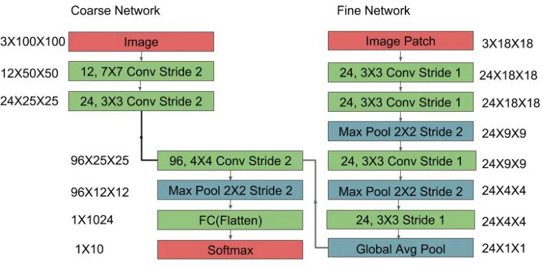
As shown in figure 3.5, a Dynamic Capacity Network consists of two sub-networks: Coarse

and Fine. First, an image is passed through the Coarse network, then runs the Fine

sub-network only for selected parts of the image based on the output of the Coarse sub-sub-network. This

arrangement enables the network to imitate human behavior. While solving this problem, humans

will first scan the image without giving much attention to the details, and then focus into the

area which looks like vegetation to know whether it is an invasive plant or not. Here Fine

sub-network generate rich features for interesting regions of the image. Finally, these Fine sub-sub-network

features replaced Coarse features to form a combined feature map at the corresponding place. This

combined feature map was used for generating the final classification scores.

3.4.1.1 Receptive Field

(37)

[image:37.612.89.484.230.424.2]

(38)

nected pixels is called the receptive field of the feature vector. The receptive field of a vector in a

feature map depends on multiple factors: the depth of convolutional layer in a deep neural network

which produced the feature map, kernel size, and stride of all the predecessor layers.

Since a Deep-learning network learns hierarchical features, the size of the receptive field

increases with the depth of the network. But, Fine and Coarse features should have the same size

of the receptive field so that both features can be merged in the combined feature map and maintain

its integrity.

3.4.1.2 Coarse Sub-Network

Here using the response of the Coarse sub-network, DCN selects a fixed number of sections

of the image to be passed through the Fine sub-network. The Coarse sub-Network learns the image

spatial regions where the task-relevant information is present. DCN uses Fine sub-network for

generating rich features for such spatial areas of the image which reduce the overall classification

loss. Here using the Coarse feature saliency matrixM is calculated which represents how much classification entropy is sensitive to a Coarse feature vector which is produced by Coarse

sub-network for a spatial region on the input image. Formally the saliency matrixM can be defined as the gradient of the entropyHwith respect to each spatial location of the Coarse feature mapc, where each location(i, j)in the feature mapcrepresents a feature vector such thatci,jRD. If the

number of target classes areCand scores produced by Coarse sub-network areocoarsethen entropy

H and saliency matrix value for a(i, j)locationMi,j can be described as:

H =−XC

l=1o

l

(39)

Mi,j= s

XD

r=1(

∂ ∂c(_i,jr) −

XC

l=1o

l

coarse.log(olcoarse))

Saliency measure encourages selecting the regions of the image which most affect the

un-certainty in the predictions. Each element in the saliency matrix represents a spatial area in the

input image. The elements with high values in the saliency matrix identify spatial regions in the

input image which affect the classification score the most.

3.4.1.3 Fine Sub-Network

The fine sub-network response is calculated for K selected regions associated with top

k values of the saliency matrix. The set of selected regions Xs is composed of K regions of size s1 ×s2. In the final combine feature map fr(x), response of Fine sub-network ff replace

values calculated from the Coarse sub-networkfcat spatial location corresponding to K regions.

Finally, the combined feature map generated by the Coarse and the Fine sub-networks was used

for generating a final classification score.

fr(X) =ri,j|(i, j)[1, s1]×[1, s2]

ri,j=   

ff(xi,j), ifxi,j Xs

(40)

3.4.2 End-to-End Training

Both sub-networks of the DCN network can be trained jointly or separately. Almahairi et al.

trained the sub-network of DCN jointly for the Cluttered MNIST dataset. In joint training process

parameters for both the Fineθf and Coarse sub-networkθcwas learned at the same time. For the

given training set D = (xi, yi); i= 1...m where each xi Rh×w is an image andyi 1, ...., C

is its corresponding label. The network parameters were learned by minimizing the cross-entropy

loss functionJusing the Stochastic Gradient Descent Algorithm [46].

J =−

m

X

i=1

log_p(yi|xi;θ)

3.5

Improved DCN for Google Street View Images

Our aim is to design a Deep Neural Network similar to DCN which can select the region of

interests from the image and replace the corresponding feature vectors in the Coarse feature

repre-sentation with Fine features for these selected regions. Almahairi et al. have designed the network

for solving Cluttered MNIST [36] and SVHN [42] datasets. In SVHN dataset each image was

con-taining a House Number with some background clutter. Here using the Coarse sub-network, DCN

identifies regions of the image where the alpha-numeric values were present. In our case, we were

focusing on designing a Coarse sub-network which identifies the region containing vegetation.

Since the features associated with roads and sky do not resemble vegetation, we do not require any

further processing of these regions through Fine sub-network. However, a similar looking invasive

and non-invasive plant may have similar feature representation, therefore, the network should use

(41)

non-invasive plants.

3.5.1 Network Architecture

We designed the Coarse and Fine sub-network with an almost equal receptive field. In Fine

sub-network, there were more convolutional layers present than Coarse sub-network. The Fine

sub-network for a region of size 224×224 produced feature vectors which replaced the feature

vector produced by the Coarse sub-network. There were fewer layers in the Coarse sub-network

but their kernel size and stride was larger than the layers in the Fine sub-network. Due to this,

both sub-networks had an almost equal receptive field size. Each value in the resultant saliency

matrix was influenced by a neighborhood of117×117pixels area. Therefore, the patch size while

calculating Fine sub-network response should be around 117× 117. We used the patch size of

224×224while calculating response from the Fine sub-network. This flexibility between patch

size and receptive field size was also observed in Almahairi et al.. It also gave the best results in

our experiment.

While designing the network, we believed that a patch size of224×224captures the full

context of an invasive plant and feature vector produced by the patch can effectively represent a unit

of the invasive plant. During our experiments, we found that the receptive field of size117×117

with a patch size of224×224produced the best results.

Since there was a lack of training data for our dataset and to avoid over-fitting, we added

batch normalization layers[47] along with convolutional layers. Batch normalization layers

(42)

[image:42.612.139.492.211.449.2]

(43)

3.5.2 Shared Computation

A Deep Convolutional Neural Network learns hierarchical features. Parameters learned

by kernels of the initial layers extracts basic features such as edge information and color. These

low-level features are applicable to both Coarse and Fine layers. Here the parameters learned by

the initial layer can be useful for both Coarse and Fine network. A7×7convolutional layer is

computationally expensive due to the relatively large size kernels. By sharing the same

convolu-tional layer between our Coarse and Fine sub-network we have significantly reduced the learning

parameters and the computation cost for our DCN model.

3.5.3 Data Scarcity Issue and Training Procedure

Here the task of Coarse sub-network is to learn features associated with a region containing

vegetation, and the task of the Fine sub-network is to produce features which can distinguish

invasive and non-invasive plants. Our dataset was not as large as the Cluttered MNIST [36] and

SVHN [42]. So training the network with our limited dataset for both networks at the same time

was a challenge. In order to deal with such a situation, we trained them separately. First, we only

trained the Fine network with Invasive and Background sub-image samples that were prepared

for our sliding window approach. Then after integrating the Fine sub-network, we trained the

entire end-to-end DCN. Such a training approach is also used by Ren et al. for training the object

detection algorithms like Faster RCNN [48]. Faster RCNN also has two sub-networks: Region

Proposal sub-network and Classification sub-network. They first trained the RPN sub-network

separately and then trained the entire network end-to-end.

In training process parameters for the Fine θf were learned. Then we locked the Fine

(44)

D= (xi_{, y}i_); _i_{= 1}_...m_{, where each}_xi_Rh×w_{is an image and}_yi₁_{, ...., C}_{is its corresponding}

label. The network parameters were learned by minimizing the class weightedwi cross-entropy

loss function J using Stochastic Gradient Descent Algorithm. We used weighted cross-entropy loss function for enabling the network to give equal importance to the samples of the minority and

majority classes while calculating lossJ.

J =−

m

X

i=1

wi.logp(y i_|

xi;θ)

If in the provided dataset the number of samples for classiisni then:

wi =

ni

PC

j=1nj

We can assume feature vectors generated by such pre-trained Fine sub-network produced

useful information about any selected regions using the saliency measurements in terms of whether

the selected region contains an invasive plant or not. After end-to-end training, the Coarse part

pro-duced higher activation for the corresponding region of the image where class relevant information

resides. Saliency matrix measures the sensitivity of overall classification entropy with respect to

these higher activation regions. By using Fine sub-network more refined representation of these

areas are produced while constructing the combined feature map.

3.5.4 Data Augmentation

We also augmented the dataset for encouraging the Coarse sub-network to identify class

relevant information by learning about the presence of invasive plants. For this, as shown in figure

3.7, we inserted the invasive plants cropped images inside non-invasive images. By doing so, the

(45)

We wanted to encourage the kernels of layers at the appropriate depth to learn parameters for

producing activation when invasive plants are present. However, we didn’t observe any significant

improvement in the performance of the network after incorporating augmented samples in the

training set. We still need to further investigate the cause of lack of improvement in performance

of the network after data augmentation, as it is also possible that final feature vector representing

[image:45.612.75.540.227.323.2]

invasive plants is not distinguishable to the feature vector generated for other plants.

(46)

Chapter 4

Results and Discussion

4.1

Evaluation Method

For invasive plants classifier we are interested in measuring:Pr(N on−nativeP hragmites|

P anorama) andPr(J apaneseKnotweed | P anorama). Therefore we are training two differ-ent classifiers for recognizing each type of invasive plants. We are using Precision and Recall

measurements for evaluating the performance of classifiers. Our objective is to develop a reliable

invasive plant classification system which can show acceptable Precision and Recall for unseen test

samples. We have compared the performance of various invasive plants classification approaches

using Precision Vs Recall curves. In a real-world, the number of images containing any invasive

plant is far less than the images containing no invasive plant. Therefore our objective is to

de-velop a classification method which keeps false positive low. Because due to a large number of

non-invasive samples, the relative number of false positive samples can be much higher than true

positive. As there is a financial cost associated with transporting machinery and people for

inva-sive plant removal to the affect areas, therefore, a large number of false positive will increase the

overall financial cost of the invasive plant removal efforts. If for an invasive plants classifier false

positive aref pand true positive aretp, then precisionP recisioncan be measured as:

Precision = tp

(47)

In order to train our models for achieving a higher precision score, we first select a classifier

which achieves a high area under the Precision-Recall curve, then we will set the classification

thresholdT hhigher for setting higher precision. For a given sample image if the classifier produces normalized scoresthen classcof the sample can be decided by:

c =   

Invasive, ifs > T h N on−Invasive, otherwise.

4.2

Off the shelf models

During our initial experiments, we trained off the shelf image classification models to

mea-sure their performance for our dataset. We also made necessary changes in the model to improve

their performance. We found that the existing state of the art CNN models was not able to produce

acceptable classification performance due to the large size of the images and object of interest

occupied relatively a small part of the image.

4.2.1 ResNet18

In general, as the number of layers in Deep Neural Network increases classification

ac-curacy ideally should also increase. But these very deep networks are prone to saturate during

training and their performance starts decreasing rapidly on the further training stages. Ideally, the

performance of a Deep Neural Network should not be affected by adding some extra layers

be-cause these newly added layers can always learn identity transformation after training. But it was

found that these layers were unable to optimally learn identity transformation. The ResNet model,

(48)

functionf0between inputxand outputy. If the network parameters arewthen:

y =f(x, w)

y =f0(x, w) +x

Here when the residual network tries to learn identity transformation, it optimizes the

pa-rameterswfor performing zero transformation.

In 2015 ResNet outperformed other object classification algorithms in terms of

classifica-tion accuracy. The network has shown higher accuracy while predicting classes for224×224size

images of the ImageNet dataset. In ImageNet dataset, the object of interest was in focus of the

camera while taking the picture. Such an arrangement helps the classification methods thereby

increasing accuracy. A ResNet model can be developed by stacking multiple residual layers. For

our experiments, we used the ResNet18 model which consists of 18 residual layers.

We performed three experiments to test the performance of the ResNet18 model by

classi-fying high-resolution Google Street View images in our dataset. For all the experiments, we trained

the model with ImageNet dataset to perform transfer learning. Initial layers of a Deep Neural

Net-work learn lower level features which are relevant to any kind of object. Therefore parameters of

the initial layers learned after pre-training of the network are also relevant to our dataset. Also, as

shown in table 4.2, the pre-trained network has performed better than not pre-trained models for

(49)

• In the first experiment, we re-sized the images of our dataset to 224 ×224 size in order

to make it similarly sized images in ImageNet dataset. Then we finetune the pre-trained

ResNet18 model with our dataset. As shown in figure 4.1, this experiment did not produce

good results. Due to the re-size, resolution of images was reduced significantly and all the

[image:49.612.110.498.223.446.2]

distinct features associated with the invasive plants were also lost.

Figure 4.1: ROC and PR curves for the finetune ResNet18 model with test images of size224×224

• In the second experiment, we finetune the pre-trained ResNet18 model while maintaining

high resolution (1400×6156) of the images. Since the model was not originally designed for

handling such high-resolution images, it wasn’t able to effectively learn the feature

associ-ated with the invasive plants. Also, the network performs a global average pooling operation

(50)

the input image, the spatial size of the final feature map was also large. When the network

performed global average pooling operation on the final feature map, any set of feature

vec-tors associated with invasive plants were also averaged with a large number of other feature

vectors. Thus the network failed to identify the invasive plants. As shown in the figure, 4.2,

[image:50.612.109.499.223.446.2]

this classifier has shown the lowest performance.

Figure 4.2: ROC and PR curves for the finetune ResNet18 model with test images of size1400×

6156

• In the final experiment, while maintaining the input image resolution high(1400×6156),

we replace the global average pooling layer with a global max-pooling layer. Such an

ar-rangement encouraged the network to assign higher values to the feature vector associated

(51)

better performance compared to the classifier trained in the second experiment but still, it

[image:51.612.113.498.151.375.2]

was not acceptable.

Figure 4.3: ROC and PR curves for the finetune modified ResNet18 model with test images of size 1400×6156

4.3

Sliding-Window

We implemented a naive approach by dividing the large images of our dataset into multiple

small sub-images of size224×224. By moving a sliding window on the high-resolution images

non-overlapping sub-images were generated. This process produced around 740 sub-images of

size224×224for an input high-resolution image of size2800×13000. Subsequently, we trained

(52)

[image:52.612.110.498.227.449.2]

(53)

As shown in figure 4.4, the trained ResNet18 sub-image classifier achieved high precision

and recall for the sub-image testing set. The ratio of invasive and background images was1 : 3in

the testing set. But for a given set of high-resolution images, the number of background sub-images

not containing invasive plants outnumbered the invasive plants sub-images by a ratio of 100 : 1.

In such a scenario, if we apply the sub-image classifier on all these sub-images then a large number

of the false positive sample will reduce the performance due to an asymmetric distribution of

sub-images in the dataset. As shown in figure 4.5, when we applied the classifier on all the sub-sub-images

generated from our original dataset, performance was reduced significantly due to a large number

[image:53.612.111.497.313.535.2]

of false positives.

Figure 4.5: ROC and PR curves for the finetune ResNet18 model with all sub-images of size 224×224

(54)

applied the algorithm 1 while generating class scores for the whole image using the scores received

for its sub-images. This algorithm assigns a score to the whole image by averaging the scores of

it’s25sub-images having the highest score for the invasive class. As shown in the figure 4.6, high

classification results were achieved by using algorithm 1. Performance of this method was further

[image:54.612.110.498.225.446.2]

improved when we used DenseNet121 as sub-image classifier.

Figure 4.6: ROC and PR curves for the algorithm 1

4.4

Dynamic Capacity Network

4.4.1 Implementation and Benchmarking of the DCN

We implemented the DCN using the Pytorch deep learning library and compared its

(55)

implementation, instead of Adam optimizer mentioned in the paper, we used a stochastic gradient

descent algorithm for training the network as the training process was relatively stable for the later

one. We also implemented two separate models of single streams equivalent to the Fine and Coarse

sub-networks of the DCN respectively. We refer to them as ”Only Fine Network” and ”Only Coarse

Network”. These models were compared with the DCN for their classification performance and

computation requirements. We found that DCN has achieved equivalent performance to the Only

Fine network and better than the Only Coarse network. The convolutional layers of the Only Fine

Network produced much finer features than the Only Coarse Network. DCN network only uses

Fine sub-network for generating feature vectors for some selected parts of the images which have

task-relevant information. We refer to these selected parts as patches.

4.4.2 Quantitative Results

Our implemented DCN was able to achieve similar results mentioned by Almahairi et al.

for Cluttered MNIST dataset. For an input image of size100×100, saliency matrix of size25×25

was generated by the DCN. We performed experiments with different number of patches k = 8,10,12,14,16,18,20. As shown in the table 4.1, with k = 14, the DCN network was able to achieve accuracy equivalent to the Only Fine Network. However, Almahairi et al. were able to

achieve the same accuracy withk = 8. DCN used less number of FLOP operation than the Only Fine Network for achieving the same results. Here DCN used the Fine sub-network for generating

feature vectors for 16 patches. On the other hand, the Only Fine Network generated feature vectors

for patches corresponding to all the625locations of the saliency matrix. Here this arrangement of

DCN reduced the FLOP operation but had an overhead of calculating saliency matrix through the

(56)

[image:56.612.150.461.104.167.2]

Table 4.1: Results for Cluttered MNIST dataset

Network Accuracy FLOPs Count

Only Coarse Network 92.5% 164×104

Only Fine Network 96.2% 550×104

DCN(K=14, patch size=18×18) 96.1% 410×104

4.4.3 Qualitative Results

We investigated the spatial location of the patches selected by the saliency matrix for

cal-culating Fine features. As we can see in the figure 4.7, elements in the saliency matrix achieved

higher values corresponding to the areas around the digits where the information about the class

(57)

[image:57.612.73.527.141.508.2]

con

(58)

4.5

Improved Dynamic Capacity Network

The improved DCN performs fewer FLOP operations than ResNet18 but it has more

train-ing parameters. Therefore performtrain-ing end-to-end traintrain-ing for high-resolution images is a memory

intensive task for the GPU. We have used Nvidia GTX 1080TI GPU with a memory limit of11GB. Due to the large size of images, the size of the computational graph created for back-propagation

was also large which requires more GPU memory than the available capacity of 11GB. Thus training the improved DCN network with full resolution image on single GPU was practically

im-possible for us. GPU memory usage can be reduced by using a small batch size for the training

algorithm. But we found that the training algorithm was not able to efficiently train the network

with a very small batch size(1, 2or 3). The training algorithm for such small batch size behaves similarly to stochastic gradient descent which is not a very effective method for training Deep

Neural Networks.

We tried to solve this problem in two ways:

• (a) We reduced the resolution of images with a margin of4×4times. This enabled us to

perform training with our limited GPU memory. Results obtained by the sliding window

approach is incomparable with the DCN because the sliding window approach has an

ad-vantage of maintaining high resolution whereas DCN was trained with reduced resolution

images. Even though the DCN network was able to identify the vegetation region of the

images using the attention mechanism, the overall performance was not as good as expected.

The low performance was due to the reduction in the resolution which resulted in the loss of

(59)

of2800×832 by performing vertical scaling the image. The proportion of vegetation, sky,

and road in sub-image was equivalent to the original image. Therefore the nature of the

images did not change. The total area of the sub-images was almost equal to the area of the

re-sized(700×3328) images used in the previous experiment. We found network attention

and performance of the improved DCN was significantly improved for the high-resolution

sub-images.

4.5.1 Quantitative Results 4.5.1.1 DCN re-size

While training the improved DCN with re-sized(700×3328) images, the attention of the

network was good as it was able to detect vegetation. But as shown in the plot 4.8, the overall

classification performance was low. In comparison to the off-the-shelves models, the improved

DCN model has achieved slightly better performance by reducing the FLOP operations

signifi-cantly. The Coarse sub-network has only six convolutional layers which are far lesser than 18

layers of ResNet18. We also found improved DCN have achieved higher performance than the

(60)

[image:60.612.111.498.226.447.2]

(61)

4.5.1.2 DCN Crop

For examining the performance of the improved DCN, we created a sub-image training and

testing dataset. We kept the ratio of invasive to non-invasive images in this dataset equivalent to the

ratio present in the original database. As shown in figure 4.9, with these arrangements improved

DCN has performed better with the high resolution cropped sub-images as compared to reduced

resolution re-sized images. Also, we observed that the attention mechanism was more effective in

[image:61.612.111.497.276.498.2]

the high-resolution images.

(62)

4.5.2 Qualitative Results

We investigated the spatial location of the patches selected by the saliency matrix for

cal-culating Fine features.

4.5.2.1 DCN re-size

While evaluating the spatial regions associated with higher saliency value, we found that

most of such region represents the area of the image where vegetation exists. Figure 4.11 shows in

blue boxes the spatial regions of the images selected for calculating fine features and the

(63)

[image:63.612.74.545.79.296.2]

(64)

4.5.2.2 DCN crop

Spatial regions of the images selected for calculating fine features are shown in figure

4.13(in blue boxes). Most of the task-relevant information -vegetation- is confined in the selected

regions. Since in this experiment we have maintained the resolution of images hence fine features

were more descriptive than the previous experiment where we resized the imaged before processing

(65)

[image:65.612.74.527.79.447.2]

Figure 4.13: Showing 25 bounding boxes of the size224×224corresponding the spatial parts of images selected as input for the Fine sub-network.

4.6

Summary

The invasive dataset presented two main challenges for all the classification methods: (a)

(66)

only occupying a small portion in the entire image. By using the Improved DCN network, FLOP

operations have significantly reduced as compared to off the shelves models. But the Improved

DCN network was not able to archive higher classification accuracy. Though the number of FLOP

operations was also less for the sliding window approach there are hidden overheads are associated

[image:66.612.129.480.240.563.2]

with this approach in terms of slicing and dicing of the images.

Table 4.2: Comparison among various methods for classifying invasive plants. All ResNet18 models are pre-trained with ImageNet dataset accept other vise mentioned.

Method PR Score ROC Score FLOPs Count Non-native Phragmites

Resnet18 re-size224×224Not pre-trained .48 .67 52×106

Resnet18 re-size224×224 .55 .70 52×106

Resnet181400×6156 .31 .46 24×109

Resnet18 max1400×6156 .43 .64 24×109

Resnet18 Sliding window2800×13312 .82 .89 38×109 Resnet18 Sliding window1400×6656 .70 .85 9×109

DCN re-size1400×6656 NA NA 9×109

DCN re-size700×3328 .47 .67 3×109

DCN crop2800×832 .72 .83 3×109

Only Coarse crop .70 .80 2×109

Japanese Knotweed

Resnet18 re-size224×224Not pre-trained .36 .63 52×106

Resnet18 re-size224×224 .43 .66 52×106

Resnet181400×6156 .31 .55 24×109

Resnet18 max1400×6156 .40 .61 24×109

Resnet18 Sliding window2800×13312 .69 .81 38×109 Resnet18 Sliding window1400×6656 .55 .77 9×109

DCN re-size700×3328 .34 .58 3×109

(67)

Chapter 5

Future Work

In our future work, we are interested in further improving the DCN network by reducing

the floating point operations and increasing the accuracy of the overall classifier. We would like to

briefly discuss our ideas for achieving these future objectives in this chapter.

5.1

Improving classification accuracy

All the Deep Neural Network based approaches we have discussed so far can be

signifi-cantly improved by acquiring more training data. We improving the classification performance for

invasive dataset we can also use separate classifier for different sessions. This can be done if we

also incorporate timestamp information into the annotation details. This will help to reduce xthe

intra-class variance of the feature space.

5.2

Reducing FLOPs

For our improved DCN network the number of floating point operations(FLOPs) can be

further substantially reduced by using Shuffle Network [6] based Bottle-Neck unit architecture

(68)

5.2.1 Bottle-Neck Unit

Inception net [49] introduced Bottle-Neck architecture for reducing the number of FLOP

in the network using1×1convolution operations. A 1×1 convolution operation only operates on

the depth of the feature maps and does not consider activation of the spatial neighborhood while

producing output feature map due to its kernel size being1×1.

A 5×5 convolutional layer, consists ofN kernels each of size 5×5, performs a large number of floating point operations. If the size on the input feature map isW× H×N then it will perform

W × H×26×N2 _{FLOPs. To reduce this large number of FLOPs Szegedy et al. came up with}

an alternative approach of applying three convolution layer instead of one.

The first layer reduces the dimensions of the input feature map. The dimension of the input

feature map is reduced by applying a 1×1 convolutional layer consisting ofM kernels, where

N > M. This operation produces an intermediate output feature map of sizeW ×H ×M by performingW ×H ×N ×M number of FLOPs. The second convolution layer with M kernel each of size5×5was applied on the intermediate feature map by performingW ×H×26×M2

number of FLOPs. Finally in order to regain the intended dimensions of output feature map, a third

1×1 convolutional layer consisting ofN kernel each of size1×1is applied. It produces final

W×H×N dimensional output feature map by performingW×H×M×N number of FLOPs. The arrangement of these three convolution layers is called bottleneck unit and it produces

equivalent feature map to the original computationally expensive 5×5 convolution layer while

(69)

5.2.2 FLOPs for various Bottle-Neck units

ResNet [4] also uses Bottle Neck architecture for cutting down the number of FLOP

oper-ations. The Bottle Neck architecture was further improved by using group convolution [5]. Group

convolution is used for distributing model over multiple GPUs. It performs depth-wise separate

convolution. By using group convolution the number of FLOP operations can be reduced. The

group convolution layer performs convolution for each group of feature maps separately.

There-fore the group convolution restricts the interaction between all the input feature maps while

per-forming convolution. As shown in figure 5.1(Center), the final 1×1 convolution of the B

Exploring Deep Neural Network Models for Classification of High-resolution Panoramas

Rochester Institute of Technology

APPROVED BY

Exploring Deep Neural Network Models for Classification of

THESIS

Exploring Deep Neural Network Models for Classification of

Acknowledgments

Table of Contents

List of Tables

Chapter 1

Invasive Plant Classification System

Chapter 2

Image Classification using Deep Learning

Chapter 3

Data transformation

Baseline Approaches

Dynamic Capacity Network

Improved DCN for Google Street View Images

Chapter 4

Off the shelf models

Sliding-Window

Dynamic Capacity Network

Improved Dynamic Capacity Network

Summary

Chapter 5

Improving classification accuracy

Reducing FLOPs