High resolution paleovalley classification from airborne electromagnetic imaging and deep neural network training using digital elevation model data

Hydrol. Earth Syst. Sci., 23, 2561–2580, 2019 https://doi.org/10.5194/hess-23-2561-2019 © Author(s) 2019. This work is distributed under the Creative Commons Attribution 4.0 License.

High-resolution paleovalley classification from airborne

electromagnetic imaging and deep neural network

training using digital elevation model data

Zhenjiao Jiang1,2, Dirk Mallants2, Luk Peeters3, Lei Gao2, Camilla Soerensen3, and Gregoire Mariethoz4 1_{Key Laboratory of Groundwater Resources and Environment, Ministry of Education, College of Environment} and Resources, Jilin University, Changchun, 130021, China

2_{CSIRO Land & Water, Locked Bag 2, Glen Osmond, SA 5064, Australia} 3_{CSIRO Mineral Resources, Locked Bag 2, Glen Osmond, SA 5064, Australia}

4_{University of Lausanne, Faculty of Geosciences and Environment, Institute of Earth Surface} Dynamics, Lausanne, Switzerland

Correspondence:Zhenjiao Jiang (jiangzhenjiao@hotmail.com) Received: 9 January 2019 – Discussion started: 21 January 2019 Accepted: 20 May 2019 – Published: 13 June 2019

Abstract. Paleovalleys are buried ancient river valleys that often form productive aquifers, especially in the semiarid and arid areas of Australia. Delineating their extent and hy-drostratigraphy is however a challenging task in groundwa-ter system characgroundwa-terization. This study developed a method-ology based on the deep learning super-resolution convolu-tional neural network (SRCNN) approach, to convert electri-cal conductivity (EC) estimates from an airborne electromag-netic (AEM) survey in South Australia to a high-resolution binary paleovalley map. The SRCNN was trained and tested with a synthetic training dataset, where valleys were gener-ated from readily available digital elevation model (DEM) data from the AEM survey area. Electrical conductivities typical of valley sediments were generated by Archie’s law, and subsequently blurred by down-sampling and bicubic in-terpolation to represent noise from the AEM survey, inver-sion and interpolation. After a model training step, the SR-CNN successfully removed such noise, and reclassified the low-resolution, converted unimodal but skewed EC values into a high-resolution paleovalley index following a bimodal distribution. The latter allows us to distinguish valley from non-valley pixels. Furthermore, a realistic spatial connectiv-ity structure of the paleovalley was predicted when compared with borehole lithology logs and a valley bottom flatness indicator. Overall the methodology permitted us to better constrain the three-dimensional paleovalley geometry from

AEM images that are becoming more widely available for groundwater prospecting.

1 Introduction

A paleovalley is the remnant of an inactive ancient river val-ley filled by unconsolidated, semi-consolidated or lithified sediments, which often have a higher porosity and perme-ability than the surrounding rocks (Jackson, 2005). Paleoval-leys are important in mineral exploration as they may con-tain remobilized gold, uranium, and heavy minerals (Hou et al., 2008) and in groundwater exploration, as they often form productive aquifers (Samadder et al., 2011; Mulligan et al., 2007; Knight et al., 2018). However, delineating the geome-try and connectivity of paleovalleys at the regional scale (tens to hundreds of kilometers) with a high resolution (tens of meters in horizontal plane) is challenging (Holzschuh, 2002; Lane, 2002). This is mainly because surface geophysical sur-veys and borehole data often do not yield the required spatial resolution and coverage to reliably and cost-effectively map connected paleovalleys at a regional scale.

horizontal resolution depends on the distance between flight lines (typically between 250 m and 30 km), which can be tai-lored to the problem at hand, while vertical resolution ranges from meters to tens of meters. Classification of geophysi-cal properties into paleovalleys and non-valley zones is most often done manually, although several methods have been developed to automate the identification of lithofacies from electrical conductivity estimates. Most of these methods as-sume a simplified petrophysical relationship between electri-cal conductivity and hydraulic parameters (e.g., porosity and permeability) (Vilhelmsen et al., 2014; Marker et al., 2015; Pollock and Cirpka, 2010). Using synthetic borehole data, Christensen et al. (2017) converted AEM data to lithofacies at a scale of kilometers by use of Markov Chain Monte Carlo and sequential indicator simulation methods.

Electrical conductivity values estimated from AEM sur-veys are subject to uncertainties introduced by variations in land cover during surveys, inversion processes, and the in-terpolation of EC values to the required resolution (Viezzoli et al., 2008; Robinson et al., 2008). Consequently, the rela-tionship between EC and lithofacies is complex and difficult to identify. In this paper, we introduce a deep-learning (neu-ral network)-based methodology (including training dataset generation, and neural network construction and training) for automatic classification of high-resolution binary paleovalley maps from AEM-derived EC data with noise.

Artificial neural networks (ANNs), which can express the complex and nonlinear relationship between input and out-puts, were previously applied for the inversion of EC values from original AEM data (Ahl, 2003) and to classify lithology from AEM-derived EC data (Gunnink et al., 2012). However, the large number of weights involved in ANN make it diffi-cult to train the network and often leads to overfitting prob-lems (Tu, 1996). Deep learning approaches based on con-volutional neural networks with sharing weights were estab-lished in 2006 (Gu et al., 2017), and are now well accepted in the field of visual recognition, speech recognition and lan-guage processes. They provide efficient high-dimensional in-terpolators that cope with multiple scales and heterogeneous information (Marcais and de Dreuzy, 2017), and have been applied in geoscience for earthquake detection based on seis-mic monitoring (Perol et al., 2018), object and disaster recog-nition from remote-sensing data (Längkvist et al., 2016; Amit et al., 2016), and mineral prospectivity evaluation by the fus-ing of different geophysical datasets (Granek, 2016; Meller et al., 2013). Furthermore, a super-resolution convolutional neural network (SRCNN) approach composed merely of convolutional layers was established to directly capture the relationship between low- and high-resolution images (Dong et al., 2016). The SRCNN was found to be accurate, robust and fast for removing noise from low-resolution images and reconstructing a super-resolution image (Hao et al., 2018; Tuna et al., 2018; Luo et al., 2017).

In this study, concepts from the SRCNN approach are used to identify paleovalleys at high spatial resolution

from a regional-scale AEM survey. The objective is to de-velop a methodology based on SRCNN to generate a high-resolution, regional-scale map of paleovalleys from low-resolution AEM-derived EC data that (1) reproduces paleo-valley connectivity and (2) accounts for noise in the EC data. The method is applied to an arid region of South Australia to identify paleovalleys at depths up to 100 m, i.e., the depth up to which the AEM-derived EC has a sufficient signal-to-noise ratio. The paper is organized as follows; Sect. 2 presents the data availability in our study area. Section 3 introduces the methodology, which is followed by performance analyses in Sect. 4. Section 5 concludes the major findings.

2 Study area and dataset

Australian landscapes are ancient, featuring the product of subdued tectonics, long-term subaerial exposure and an ex-tremely limited extent of Quaternary glaciation. This often manifests itself in an extensive paleovalley network with deep weathering profiles and thick accumulation of uncon-solidated alluvium and colluvium. The widespread paleoval-ley networks in today’s arid landscape are remnants of the Early Cenozoic inset valleys with Tertiary sedimentary in-fill and a thin and variable Quaternary cover (Magee, 2009). In the intracontinental Cenozoic sedimentary basins, paleo-valley infill sediments typically consist of Eocene sediments overlain by more finely grained sediments of Oligocene to Miocene age. The Eocene sediments are dominantly coarsely grained fluvial sands and basal gravels, deposited under wet climatic conditions. The Oligocene to Miocene sediments were deposited by relatively lower-energy drainage systems under drier climatic conditions. During the Quaternary, eo-lian sediments with maximum observed thickness of 15 m covered portions of the paleovalleys at a time when fluvial or lacustrine deposition had ceased (Magee, 2009).

This study focuses on the Anangu Pitjantjatjara Yankunyt-jatjara (APY) lands, which are part of the Musgrave province in northern South Australia (Fig. 1). This area features an arid climate with very low and unreliable rainfall averaging about 230 mm yr−1(Jones et al., 2009). However, an exten-sive paleovalley system with sedimentary faces aligning with the Cenozoic sedimentary basins above represents a shal-low dynamic groundwater system exhibiting reliable water resources for local communities and mining (English et al., 2012; Munday et al., 2013).

Within the study area 128 bores, drilled between 1970 and 2018, with lithological information were retrieved from the South Australia Government WaterConnect database (https:// www.waterconnect.sa.gov.au/Pages/Home.aspx, last access: 3 January 2019). Three lithological classes were derived from the logs.

Z. Jiang et al.: High-resolution paleovalley classification by deep learning 2563

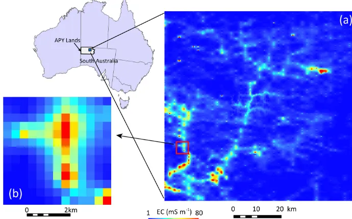
Figure 1. (a)Electrical conductivity at 100 m depth ranging from 1 to 80 mS m−1, as interpreted from airborne electromagnetic surveys in the Anangu Pitjantjatjara Yankunytjatjara (APY) lands, Australia;(b)inset shows details of EC map at a spatial resolution of 400 m×400 m (Soerensen et al., 2016).

2. Alluvium (sediments in paleovalleys). Basement cov-ered with more than 15 m of unconsolidated sediments consisting of sand and gravel with minor silt and clay, showing indication of alluvial sediment transport. 3. Transition. Basement covered with up to 15 m of eolian

sands or lacustrine sediments consisting of silt and clay with minor amounts of sand or gravel, showing limited indication of transport.

While the information content in these logs was often lim-ited, they provided independent lithological data to verify the predicted paleovalley network in this study (see further).

Two AEM surveys were flown in the APY lands in 2016, covering a total area of 33 500 km2and featuring a line spac-ing of 2 km in the north–south direction (Soerensen et al., 2016). An area 80 km by 80 km in a central-east section of the APY lands is selected and used to test mapping paleoval-leys based on a SRCNN analysis of electrical conductivity (EC) generated from the AEM survey (Fig. 1). In this area, the AEM survey was undertaken using the helicopter-borne SkyTEM312FAST system (Soerensen et al., 2016). The aver-aging trapezoidal filter was used to reduce the noise in low-and high-moment amplitude response data. Aarhus Work-bench software was used to invert AEM data to obtain EC (Auken et al., 2009, 2014). In a final step, ordinary kriging was used to interpolate EC values to a spatial resolution of 400 m×400 m in the horizontal plane and 10 m in the verti-cal cross section (Ley-Cooper and Munday, 2013; Soerensen et al., 2016). The constraint on the lateral resolution of the AEM data was determined by the line spacing of the sur-vey (2 km). In the APY lands, it was gridded to a cell size

of a fifth of the line spacing (i.e., 400 m), to maintain the fi-delity. The depth interval is commonly between 5 and 10 m increasing exponentially with depth because AEM is a diffu-sive technology (Yang et al., 2013; Spies, 1989). In the APY lands the vertical resolution is 10 m for the first 100 m depth interval to avoid generating too many interval conductivity slices. Only the EC values in the first 10 depth slices, up to 100 m depth, are used in this study to construct the binary paleovalley pattern per slice, which are then stacked up to a quasi-3-D image of the paleovalley.

Bulk electrical conductivity of the subsurface depends on both the solid phase (i.e., the rock mass) and the liquid phase (i.e., soil water and groundwater). It is further influenced by the porosity, tortuosity of the pore space and degree of water saturation. Unweathered rocks are generally a poor electrical conductor with EC values typically less than 1 mS m−1 for igneous and metamorphic rock, and 1 to 1000 mS m−1 for regolith (e.g., gravel, sand, silt and clay) (Lane, 2002); saline groundwater with a salinity level similar to seawater has an EC of around 3000–5000 mS m−1, while freshwater EC is up to 150 mS m−1(Lane, 2002; Rhoades et al., 1976; Purvance and Andricevic, 2000).

the valley and non-valley lithologies, and thus only EC is used to distinguish paleovalleys from surrounding basement. However, due to the data smoothing methods used during in-version of the AEM data and EC interpolation, and the con-tinuous variation in water salinity near the interface between paleovalley and fractured bedrocks, the resulting EC values vary continuously (Fig. 1b), which makes the boundary be-tween valley and non-valley lithologies rather diffuse. Our novel methodology allows us to automatically identify the boundaries between valley and non-valley lithologies based on convolutional neural networks.

3 Methodology

The method developed in the present study to identify pale-ovalleys is comprised of three key steps. (1) A deep neural network training dataset is generated by creating synthetic paleovalley networks from a digital elevation model (DEM) of the study area; the paleovalley network is converted to EC values by applying Archie’s law (see further) to the water-bearing formations, while EC values for the non-valley zone composed of fractured bedrock are obtained as a volume-weighted average of EC values of rock and fluid components; (2) the SRCNN is trained and validated using the synthetic EC and corresponding paleovalleys to remove noise and es-tablish a nonlinear relationship between the EC image and paleovalley image; (3) the SRCNN is then applied to predict the paleovalley in the APY lands based on measured AEM data. The algorithm of training dataset generation and SR-CNN and the performance metrics to evaluate SRSR-CNN pale-ovalley classification are described in detail below.

3.1 Synthetic training data generation

Australia is well known for its relative tectonic stability and is a stable continent located in an intraplate position. The paleovalley networks are coherent, dominantly dendritic, and largely concordant with modern topographic expres-sion (Magee, 2009). Although paleovalleys in the arid zone are partly covered by Quaternary eolian deposits, the to-pographic expression of the paleovalley pattern is still evi-dent in high-resolution digital elevation model (DEM) data (Magee, 2009). In the APY lands, crustal architecture has been preserved since the Cenozoic, and it is considered to have been unaffected by later tectonic events (Drexel and Preiss, 1995). Previous studies in the study area have considered that the paleovalleys are coincident with topo-graphic lows that characterize the contemporary landscape, with AEM images being particularly useful for locating the position of the deeper portions of the older valley system (Munday et al., 2013). It is thus assumed that the present-day valley pattern indicated by topographic lows in the study area is comparable to the paleovalley pattern according to the principle of uniformitarianism (Simpson, 1970), but shifts in

valley width, orientation and connectivity between present-day valley and paleovalley are allowed. Following this prin-ciple, we generate a synthetic paleovalley image based on a digital elevation model (DEM).

First, a DEM of the study area with a resolution of 30 m×30 m (https://earthexplorer.usgs.gov/, last access: 23 December 2018) is used to generate 15 sets of paleovalley images, mimicking paleovalleys of various spatial densities and width over an area of 80 km×80 km based on the hydro-logical analysis in ArcGIS (Fig. 2a) (details in Maidment and Morehouse, 2002). For convenience in the subsequent neural network operation, each resulting valley image is downscaled by the bicubic interpolation method to contain 800×800 pix-els with spatial resolution of 100 m. Valley widths range from 1 to 10 pixels (i.e., 100 to 1000 m). The 15 images generated from the DEM were rotated between zero and 360◦and ran-domly cropped into 20 000 small training images with a size of 50×50 pixels (Fig. 2b). Thus, the potential differences in the width and orientation of present-day valley and paleoval-ley induced by several uncertain factors, e.g., variation in the river discharge and geomorphology, can be addressed in the training images. The recombination of small training images allows recreation of valley patterns beyond those 15 full-size images generated from DEM data. A broad range of likely paleovalley patterns at varying principle orientations, widths and connectivity are available in the SRCNN training image pool.

The properties in the porous paleovalley sediments are then converted to EC values using Archie’s law (Archie, 1942):

R=R0θ−m, (1)

whereRis the electrical resistivity of the water-bearing for-mation (m),R0is the electrical resistivity of the pore water relating to water salinity (m),θ is the porosity andmis a constant relating to the lithology (with value ranging from 1.8 to 2.0) (Worthington, 1993). Electrical conductivity val-ues are calculated as the inverse of resistivity valval-ues (i.e., EC=1/R). In the present study area,R0 is considered to range from 1.4 to 1.7m, corresponding to water salinities of 3000 to 6000 mg L−1 _{(Varma, 2012), whileθ is} consid-ered to range from 10 % to 30 % (Taylor et al., 2015; Varma, 2012). As a result, paleovalley EC values are estimated to be within the range of 6 to 80 mS m−1, which is in the range of AEM-derived EC values in Fig. 1.

In contrast, the non-paleovalley zone is predominantly fractured rock with solid-phase EC values <1 mS m−1, characteristic porosity of <1 % and fluid salinity val-ues of <150 mS m−1 EC (1000 mg L−1) (Olhoeft, 1981; Parkhomenko, 2012). The bulk EC values in the non-paleovalley zones were estimated as the volume-weighted average of EC in fractured rock and fluid, following

Z. Jiang et al.: High-resolution paleovalley classification by deep learning 2565

where EC is the bulk electrical conductivity, ECs is the EC value of rocks, ECf is the EC of fluid andϕ is the ratio of fracture void volume to total volume. The resulting bulk EC values are lower than 2.5 mS m−1. Again, these synthetic EC values are similar to the AEM-derived values for the pre-sumed fractured bedrock areas (Fig. 1).

Furthermore, to represent the effects from data smoothing and inherent noise associated with the AEM survey, inversion and data interpolation, artificial noise is generated by ran-domly sampling EC values in the non-paleovalley zones (fol-lowing a uniform distribution ranging from 1 to 10 mS m−1) and in the paleovalley zones (following a uniform distribu-tion ranging from 6 and 80 mS m−1). It is also noted that the upper-limit EC values in fractured bedrock areas are en-larged artificially from 2.5 to 10 mS m−1, to assure that in the training images paleovalley and non-paleovalley zones over-lap in EC by 4 mS m−1_{(5 % of the total range of EC values} between 1 and 80 mS m−1_{) (Fig. 2c). The SRCNN can then} learn to identify this overlap in EC between paleovalley and non-valley zones. However, Appendix A1 shows that setting the overlapping size in EC too large results in the trained SRCNN overestimating the extent of the non-valley zones, which make the predicted paleovalleys disconnected.

The overlap in EC near the boundary between paleoval-ley and non-valpaleoval-ley is further enhanced by data smoothing: the resultant EC images of 50×50 pixels is first downscaled into images with a smaller number of pixels, i.e., 40×40 (20 000 images), 30×30 (20 000 images), 20×20 (20 000 im-ages) and 10×10 (20 000 images) pixels, respectively, by nearest-neighbor interpolation. These resulting 80 000 im-ages are then upscaled by bicubic interpolation to yield blurred images with the original resolution of 50×50 pix-els (Fig. 2d). In this manner, the EC values in the paleovalley and non-paleovalley zones are smoothed and the boundary between paleovalley and non-paleovalley becomes blurred.

We then randomly selected 70 000 EC images from a total of 100 000 images, composed of 20 000 pre-interpolation EC images (Fig. 2c) and 80 000 reconstructed blurred EC images (Fig. 2d) with a size of 50×50 pixels, as input to the neural network (see further), with the original synthetic paleovalley images (pixel code 1) and non-paleovalley (pixel code 0) pix-els (Fig. 2b) as output. From the random set of 70 000 im-ages, 60 000 pairs of EC (Fig. 2c and d, as input) and pale-ovalley images (Fig. 2b, as output) are used as a “training dataset” for training the SRCNN. A total of 6000 pairs are used as “validation dataset” for validation and another 4000 are used as “testing dataset” to demonstrate the performance of the trained SRCNN in removing the noise in EC images and lithofacies (paleovalley and non-paleovalley) classifica-tion.

3.2 SRCNN algorithm

To quantify the relationship between EC images and pa-leovalley images, the super-resolution convolutional neural

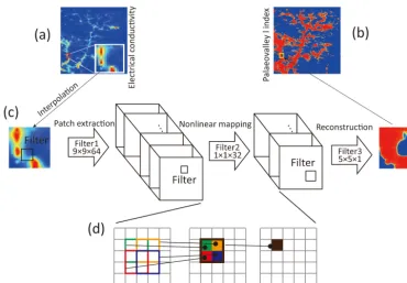
network (SRCNN) algorithm is employed. Neural networks are regression models that provide a general way of identi-fying nonlinear relationships between two sets of variables (Bishop, 1996; Moysey et al., 2003), where one set of vari-ables is considered to be the input (herein electrical conduc-tivity) and another is a network output (binary paleovalley). The SRCNN algorithm can directly train the relationship be-tween a low-resolution (input) and a high-resolution image (output) (Dong et al., 2016). A typical SRCNN is composed of three convolution layers (Fig. 3), representing patch ex-traction and representation, nonlinear mapping, and recon-struction.

In the patch extraction and representation layer, the input is a normalized 50×50 pixel EC image, which is operated by a convolution process:

H1(X)=max0,DXW1E+b1, (3) whereHrepresents the output images,<>is the convolu-tion operator,Xrepresents the input EC image, andWand brepresent the weight filter and bias, respectively.W1 cor-responds ton1filters with a size off1×f1andb1is ann1 -dimensional vector. After convolution,H1 _containsn

1 gen-erated 50×50 pixel images that are input into the nonlinear mapping layer. It is then convoluted by

H2H1=max0,DH1W2E+b2 (4) to generateH2composed byn250×50 pixel images, where W2containsn2filters with a size ofn1×f2×f2andb2is a n1×n2matrix.

Finally, an output paleovalley index (with values proaching zero indicating a non-valley pixel and values ap-proaching unity indicating a paleovalley pixel) can be recon-structed fromH2by

H3H2=GDH2W3E+b3. (5) H3contains one 50×50 pixel paleovalley index image, and W3contains one filter with a size ofn2×f3×f3andb2is an2×1 matrix.G(·)is a sigmoid function to assist the pa-leovalley classification and accelerate the training processes, which is written as

Z. Jiang et al.: High-resolution paleovalley classification by deep learning 2567

Figure 3.Algorithm of converting(a)low-resolution EC image to(b)high-resolution paleovalley image based on(c)the super-resolution convolutional neural network.(d)Convolutional processes of data from an input image to an output image by a filter with a size of 2, moving through the input image 1 pixel at the time.

illustrated in Fig. 3d, in each calculation, the EC values in the filter are convoluted to form a value at a single pixel in the output image. An EC image convoluted by the filter with the size of 2 and stride of 1 (i.e., filter moving 1 pixel at the time) and one hidden layer, leads to a paleovalley index at 1 pixel of the output image that relates to EC values from 3×3 pix-els in the input image. In this example, the spatial correlation scale able to be addressed is equal to 3 pixels multiplied by the size of each pixel (meter). In addition, the width of each layer determines the degree of the nonlinear relationship be-tween input and output, while the depth of the network af-fects both the spatial correlation length and the nonlinearity (see further in Appendix A3).

The initial weight values are randomly generated, follow-ing a standard normal distribution, while initial bias values are given as 0.1. Both weight and bias values for each of the three convolutional neural network layers are optimized simultaneously using the adaptive moment estimation algo-rithm (Kingma and Ba, 2014) to minimize the loss function,

L, which is defined as the mean sum of squared residuals:

LW1,W2,W3,b1,b2,b3= 1

N

N

X

i=1 H

3_−Y 2

, (7)

where Yis the known binary paleovalley pattern (0 repre-sents non-paleovalley, 1 corresponds to the paleovalley) in the training data, and N is the number of image pixels in each training.

3.3 Performance metrics of the SRCNN algorithm To verify the performance of the SRCNN, the following im-age quality indices are calculated.

1. Peak signal-to-noise ratio (PSNR) (Wang and Bovik, 2002):

PSNR= −10log₁₀

"

1

N

N

X

i=1

(eYi−Yi)2

#

, (8)

whereY represents the synthetic binary paleovalley in-dex generated from the DEM (0 for non-paleovalley and 1 for paleovalley) (Fig. 2b) andYeis the calculated

pale-ovalley index (Eq. 5) from SRCNN using EC images as input, and the term between brackets is the mean square error. PSNR is a traditional approach to image quality assessment. A high PSNR represents a high-quality pa-leovalley generation; e.g., a PSNR=20 value is equiv-alent to a mean-square error of 0.01.

2. Structure similarity index (SSIM) (Wang et al., 2004): SSIM= 2µYµeY+ε

µ2_Y+µ2

e Y+ε

·2cov Y,Ye

+ε

σ_Y2+σ2

e Y+ε

, (9)

between a reference and distorted image. It ranges theo-retically from 0 to 1.0. The higher the SSIM, the higher the resolution of the paleovalley network being recon-structed.

3. Connectivity function (Pardo-Igúzquiza and Dowd, 2003; Renard and Allard, 2013):

τ (h)=N (u↔u+h|u, u+h∈S)

N (u, u+h∈S) , (10)

whereN (uu+h∈S)is the number of paleovalley pix-els in a certain direction within the distance h, while

N (u↔u+h|uu+h∈S) is the number of connected paleovalley pixels in this direction. It ranges from 0 to 1.0, and high values indicate a strong spatial connectiv-ity.

4 Results and discussion

We here (1) monitor both PSNR and SSIM between the pale-ovalley index generated from SRCNN and DEM for 60 000 training and 6000 validation datasets to test for the overfitting problem; (2) generate paleovalley index maps from synthetic EC images in 4000 testing datasets to demonstrate the per-formance of SRCNN in identifying the noise in EC images and classification and recreate the connectivity of the pale-ovalley; (3) infer binary paleovalley maps by applying the trained SRCNN to the AEM-based EC values in the study area; and (4) compare the resulting paleovalley image with borehole lithology logs and existing paleovalley indicators, i.e., multiple-resolution valley bottom flatness.

4.1 Training and preliminary testing

The training dataset composed of 60 000 pairs of EC and valley images in Fig. 2 is divided into 1200 batches (inner number of iterations) with each batch containing 50 images. The epoch (outer number of iterations) is set to 5, and the 60 000 training image pairs are resorted at the beginning of each epoch. In this scenario, weights and biases in the SR-CNN are updated by 6000 iterations (5×1200), according to the loss function calculated based on 50 pairs of images in each batch.

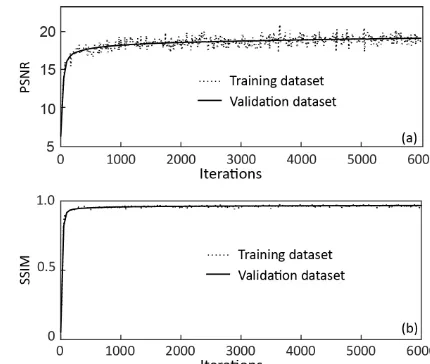
After each iteration, the PSNR (Eq. 8) and SSIM (Eq. 9) for 50 training images in each batch are calculated (Fig. 4a and b). Moreover, the PSNR and SSIM for 6000 validation images are calculated for every 50 iterations. It is illustrated that PSNR for each training batch fluctuates near 18 (which corresponds to a mean-square error of 0.015 based on Eq. 8), while the SSIM stabilizes at 0.96. The PSNR and SSIM val-ues for the validation images agree well with those of the training images. This suggests that the SRCNN is sufficiently trained to recreate the paleovalley with a high accuracy with-out overfitting problems, and importantly preserving struc-tural similarity.

Figure 4. (a)PSNR and(b)SSIM values between paleovalley in-dex generated from SRCNN and DEM recorded for both training (60 000 images) and validation (6000 images) datasets. For SRCNN training 50 images are used per iteration.

4.2 Performance of SRCNN for noise removal,

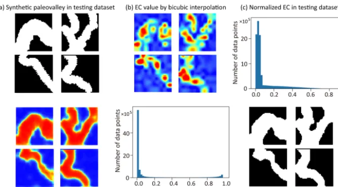
lithofacies classification and recreating connectivity The trained SRCNN is then applied to generate paleovalley images based on 4000 testing EC images; we here randomly selected four images to demonstrate the ability of SRCNN. The synthetic paleovalley images from DEM and their corre-sponding blurred EC images are illustrated in Fig. 5a and b, respectively. The histogram of EC values for all 4000 im-ages (each containing 50×50 pixels) in the testing dataset follows a unimodal, right-skewed distribution (Fig. 5c). It is not trivial to define an EC threshold value from such uni-modal distribution that can be used to distinguish the pale-ovalley and non-palepale-ovalley cells from Fig. 5b. After cali-bration of the SRCNN, a paleovalley index map is obtained (Fig. 5d). However, the histogram of the resultant paleoval-ley index displays a bimodal behavior, with peaks centered at 0 and 1 (Fig. 5e). By selecting a threshold paleovalley index value of 0.5, the paleovalley and the non-paleovalley data can be differentiated and converted to a binary paleovalley map (Fig. 5f). The resultant paleovalleys compare well with the reference (i.e., synthetic) paleovalleys in Fig. 5a. The selec-tion of a threshold paleovalley index in the range of 0.2 to 0.8 does not have a significant influence on the resultant binary paleovalley pattern.

Z. Jiang et al.: High-resolution paleovalley classification by deep learning 2569

Figure 5. (a)DEM-generated synthetic paleovalley used as reference image in testing the SRCNN;(b)normalized electrical conductivities corresponding to the paleovalleys following (c)a skewed distribution (based on 4000 images in the test dataset).(d) Paleovalley index generated through processing EC images via the SRCNN;(e)bimodal distribution of paleovalley index (based on 4000 images in the test dataset);(f)the paleovalley index map converted into a binary paleovalley map by arbitrarily selecting the paleovalley index threshold as 0.5.

and (3) it classifies the paleovalley and non-paleovalley com-ponents, which allows the selection of a threshold index to define paleovalley and non-paleovalley zones.

4.3 SRCNN performance under different image resolutions

The next synthetic example considers 400 m wide synthetic paleovalleys generated in ArcGIS from the DEM in the zone about 60 km southwest of the study area in Fig. 1a. The total extent of each synthetic paleovalley image is 80 km by 80 km, with the resolutions ranging from 200×200 to 2000×2000 pixels. The paleovalley image (Fig. 6e) with 200×200 pixels is converted to EC values based on Archie’s law (Fig. 6a), with EC values overlapping by 2.5 % between paleovalley and non-paleovalley zones. This low-resolution EC image is upscaled to a high-resolution EC image by bicu-bic interpolation (Fig. 6b), which is then cropped to images of 50×50 pixels and used as an input image for the SR-CNN. Subsequently, the paleovalley index and histogram at different resolutions are obtained (Fig. 6c). Following the histogram of the paleovalley index, it is easy to select an ar-bitrary threshold in the range 0.25–0.8 to convert the paleo-valley index (Fig. 6c) to a binary paleopaleo-valley (Fig. 6d). The choice of threshold in this range does not affect the resultant binary paleovalley pattern, as after SRCNN processing, the paleovalley index is already well grouped. The calculation of the paleovalley index at the resolution of 2000×2000 pixels takes 52 s.

It is worth noting that as the resolution of the resultant paleovalley increases, the PSNR and SSIM goodness-of-fit metrics and connectivity do not change significantly (Fig. 7). Both PSNR and SSIM increase with the resolution from

200×200 to 800×800 pixels because the bicubic interpo-lation smoothes the EC values and reduces the noise in EC values. When the image resolution further increases from 800 to 2000, PSNR degrades weakly from 18.48 to 17.09 (corre-sponding to an increase in mean-square error from 0.014 to 0.019) and, similarly, SSIM decreases from 0.8919 to 0.8522. Because each image has a fixed extent of 80 m×80 km, as the resolution increases, the distance between pixels and the real geological scale of 50×50 pixel images decreases. When the resolution increases from 200×200 to 2000× 2000 pixels, the distance between pixels decreases from 400 to 40 m and the real scale of each training image decreases from 20 km×20 km to 2 km×2 km. When training the SR-CNN, the distance between pixels was not accounted for. The training images in the training dataset include images without any paleovalley and images being fully occupied by the paleovalleys, with the narrowest paleovalley occupying merely 1 pixel. These paleovalley patterns are unrelated to the real scale of the training image, i.e., across the range from 20 km×20 km to 2 km×2 km. Thus, the trained SR-CNN works well to infer paleovalleys across different reso-lutions and scales.

4.4 Application to APY lands AEM data

Figure 6. Workflow for generating a binary paleovalley map:(a)upscaling the 200×200 pixel electrical conductivity image to (b) a 2000×2000 pixel image using bicubic interpolation; (c) SRCNN processing; (d) generating a binary paleovalley at resolution of 2000×2000 pixels;(e)binary paleovalley with characteristics comparable to the original synthetic paleovalley.

will apply the methodology to the AEM images from all 10 depths to extract specific information on the depth structure of the paleovalley network.

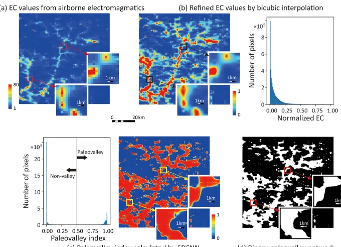
Figure 8 summarizes how the previously trained SRCNN successfully converts the low-resolution EC values resulting from an AEM survey to a binary map composed of paleo-valleys and non-paleovalley areas (Fig. 8a). First, the bicubic interpolation generates a high-resolution EC image charac-terized by a right-skewed distribution of normalized EC val-ues (Fig. 8b). This map does not yet allow a clear differentia-tion of the paleovalley from the surrounding fractured rocks. However, once we apply the SRCNN, a paleovalley index map with the paleovalley index following a binomial distri-bution is produced (Fig. 8c). Selecting an appropriate index (0.5 here) separates paleovalley from non-paleovalley pixels (Fig. 8d).

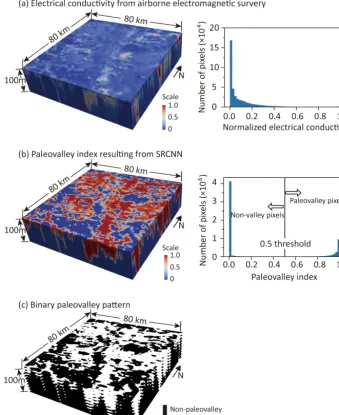
Inversion of AEM-derived EC maps at 10 depths within the first 100 m below the land surface (at 10 m intervals) is shown in Fig. 9a. EC values available at 10 layers are con-verted to binary paleovalley images by SRCNN, based on the premise that both the paleovalley pattern and bulk elec-trical conductivity from the 100 m depth interval can be rep-resented in training images. As shown in Fig. 9a, normalized EC values derived from the AEM survey are characterized by a right-skewed distribution. However, once we apply the SRCNN, the resulting paleovalley index map (Fig. 9b) dis-plays a binomial distribution of paleovalley indices. Select-ing an appropriate index (0.5 here) generates a regional-scale 3-D binary paleovalley image with a horizontal resolution of 40 m and vertical resolution of 10 m (Fig. 9c).

In the subsequent discussion we first test the derived pale-ovalley map with independent, yet limited, borehole data and auxiliary land surface maps. Next we extract further

informa-tion from Fig. 9c about the depth structure of the paleovalleys to better constrain the areas for groundwater prospection.

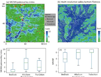
To compare the paleovalley map (Fig. 9c) with borehole logs and an alternative indictor of the location of valley in the land surface (i.e., the multiple resolution valley bottom flat-ness index; Gallant and Dowling, 2003), we aggregated the 10 depth slices of Fig. 9c into a 2-D paleovalley index map, with values ranging from zero (i.e., no paleovalley within the 10 depth layers) to 10 (i.e., paleovalley detected across all depth layers) (Fig. 10a).

The resulting paleovalley index map in Fig. 10a is first compared to the Multiple Resolution Valley Bottom Flatness (MRVBF) index in Fig. 10b, which was originally calculated by Gallant and Dowling (2003) based on a digital elevation model with a spatial resolution of 100 m. High MRVBF val-ues indicate a high probability of deposition of alluvium sed-iments. It was used by Munday et al. (2013), together with field observations of regolith, to obtain a hydrofacies map (black line in Fig. 10a). A comparison of the contours of the SRCNN paleovalley index 10 and 6 with the MRVBF index shows the emergence of similar patterns (Fig. 10a and b). While this confirms that the SRCNN paleovalley index map is not inconsistent with the MRVBF index, the latter contains insufficient information for testing the paleovalley map.

Z. Jiang et al.: High-resolution paleovalley classification by deep learning 2571

Figure 7.The PSNR, SSIM and connectivity of paleovalleys generated by SRCNN for different resolutions of upscaling the low-resolution EC image to a high-resolution binary paleovalley.

Figure 8.Steps to derive a binary paleovalley network in an 80 km×80 km region in APY lands, Australia.(a)Raw EC map at a depth of 100 m;(b)EC map after bicubic interpolation;(c)paleovalley channel index map after application of the trained SRCNN method;(d)binary paleovalley map.

In contrast, the AEM survey and the paleovalley classi-fication based on automatic neural networks in this study have improved our capability of identifying the position of paleovalleys. The boxplot of Fig. 10c shows that the bore-holes classified as “alluvium” correspond to a higher median SRCNN paleovalley index of 4, compared to the two other lithology classes of median paleovalley index of 0 and 2,

Figure 9. (a)Rescaled AEM-derived EC map and corresponding histogram of normalized EC values within the depth interval of 100 m in an 80 km×80 km region in APY lands, Australia;(b)paleovalley indices map and corresponding histogram after application of the trained SRCNN;(c)binary paleovalley map.

100 km2), there is a clear trend that bores in alluvial sedi-ments correspond to the areas with the highest SRCNN in-dex. It is reasonable to assume that these alluvial sediments represent paleovalleys, although the lithological classifica-tion did not provide this level of detail. However, for 11 al-luvial boreholes, only a low corresponding paleovalley index of<2 was identified. This may be due to the limited litholog-ical and sedimentary information captured by the downhole logs, which were mainly recorded in the 1970s with limited description of the subsurface environment. The same is true for the boreholes in bedrock and transition zones, which may have been misclassified due to insufficient data.

The paleovalley network shown in Fig. 10a is based on an analysis of 10 depth layers and hence gives greater

confi-dence about the location of deep paleovalleys than the anal-ysis of a single-depth paleovalley map (Fig. 8). A significant proportion of the image has a maximum index of 10, mean-ing that a paleovalley has been detected throughout the full investigation depth. This is thus an area with a high certainty (i.e., all pixels with index 10 have 10 layers identified as pa-leovalley) that at least a 100 m deep paleovalley is present. For the subsequent indices, e.g., 8, 6 and 4, at least eight, six and four depth layers with a paleovalley were identified, respectively.

Z. Jiang et al.: High-resolution paleovalley classification by deep learning 2573

Figure 10. (a)SRCNN paleovalley index by aggregating the binary paleovalley in the vertical direction within 100 m;(b)multiple resolution valley bottom flatness (MRVBF) indicating the position of alluvium sediment accumulation. The black lines show the boundary between paleovalley and non-paleovalley interpreted from(b), while the white lines represent the contour lines of SRCNN paleovalley index from(a). The boxplot of SRCNN paleovalley index(c)and MRVBF(d)with respect to the borehole logs showing bedrock, alluvium and transition between bedrock and alluvium.

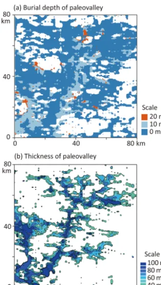
of the paleovalleys are buried up to a depth of 10 to 20 m, which cannot be observed directly from the land surface, but can be revealed by the methodology proposed in this work based on geophysical prospecting (here 3-D AEM data).

We finally calculate the thickness of paleovalley lay-ers (potentially representing the thickness of an alluvium aquifer) from the 10 depth layers with paleovalley indices. As a result, the thickness of the paleovalley calculated by the distance between bottom (lowest part) and top (uppermost part) of the paleovalley (Fig. 11b) is identical to the paleoval-ley index (Fig. 10b) multiplied by the layer thickness of 10 m. This indicates that except for those pixels that were shown to have a 10 to 20 m cover of non-paleovalley sediments (see burial depth in Fig. 11a), all other pixels had uninterrupted paleovalley layers starting from the land surface. In those pa-leovalley zones without surface sediment cover, the SRCNN paleovalley indices 8, 6 and 4 of Fig. 10a are representative for uninterrupted paleovalley sediments in the depth intervals 0–80, 0–60 and 0–40 m, respectively.

Note that in Fig. 10a at any pixel with given paleovalley in-dexn(from 0 to 10), the probability of findingnconsecutive paleovalley layers can be inferred; in our test case area this was 100 % everywhere – except for the buried pixels with 10 to 20 m cover of non-paleovalley sediments – as no in-terruption was detected in the sequence of paleovalley layers

identified. This demonstrates that despite expected vertical lithological heterogeneities within paleovalleys (Knight et al., 2018), AEM images combined with our SRCNN method-ology are able to identify and differentiate a broad series of sediments that make up a paleovalley from the surrounding bedrock. The SRCNN paleovalley index map thus provides an improved tool for groundwater prospectivity.

5 Conclusions

su-Figure 11. (a) Burial depth and thickness (>40 m) of the allu-vium sediments in paleovalleys inferred from the 3-D binary val-ley image of Fig. 9c with a 10 m vertical resolution. The hollow zone in(a)represents no identified paleovalleys within the depth of 100 m in the study area.

pervised learning, SRCNN successfully removed noise from AEM-derived electrical conductivity (EC) data and classi-fied EC values into two separate paleovalley index groups: one close to zero (the non-paleovalley areas) and another one near unity (the paleovalley areas). The resultant bimodal his-togram of paleovalley index was then used to select threshold values to convert paleovalley indices to a binary paleoval-ley and non-paleovalpaleoval-ley image. SRCNN can accommodate the spatial correlation between EC and paleovalley index by moving filters to recreate the connectivity of the paleovalley network. Moreover, the high-resolution of paleovalley pat-terns can be inferred from low-resolution EC images via SR-CNN, as long as their relationship is addressed in the training image dataset.

However, there are several limitations to the method that require more work. In applying the SRCNN methodology, only EC images were used here to identify the paleoval-ley network. In those areas where paleovalpaleoval-ley and non-paleovalley zones contain fluid with similar salinity, lead-ing to similar bulk EC values, more geophysical information, e.g., gravity and magnetics, can be used as inputs in SRCNN to distinguish the position of the paleovalley. To generate a large training image pool, SRCNN was based on 2-D training images derived from DEM data. The trained SRCNNs were

employed at different depth slices independently, where they were stacked up into a quasi-3-D paleovalley image. How-ever, the vertical relationship between EC and paleovalley index could not be addressed. In the future, the 3-D paleo-valley patterns in the training dataset could be generated by process-based methods (e.g., sedimentary processes model-ing) or multiple geostatistical approaches, and 3-D images could be used in SRCNN to address horizontal and vertical correlations between EC and paleovalley index simultane-ously. In addition, when applying the SRCNN methodology to a new study area, the training images need to be updated according to the factors influencing the relationship between target geobody and electrical conductivities (i.e., porosity, water content and sediment components in Archie’s equa-tion).

Z. Jiang et al.: High-resolution paleovalley classification by deep learning 2575 Appendix A: Robustness testing of the SRCNN

methodology

The neural network settings used in this study were as fol-lows: f1=9, f2=1 and f3=5 and n1=64,n2=32 and n3=1, where f represents the filter size and nrepresents number of output images from layer 1, layer 2 and layer 3, re-spectively, the size of input image is 50, and the overlapping size of EC values between paleovalley and non-paleovalley zone is 5 %. We now modify each of these parameters in-dividually while fixing the others to investigate the robust-ness of the SRCNN as quantified by the performance metrics PSNR, SSIM and connectivity.

A1 Overlapping size

In this study, an overlap in EC values between paleovalley and non-paleovalley zones is induced to reflect impact by factors such as noise and smoothing in the AEM data inter-pretation and interpolation; the maximum overlapping size discussed is 5 % of the range of EC values (1–80 mS m−1).

As shown in Fig. A1, the EC overlap between non-paleovalley and non-paleovalley zones in the training dataset only alters the speed at which the metrics PSNR and SSIM stabi-lize, but it does not affect the final PSNR and SSIM values. When the overlap size in the training dataset is comparable to that in the testing dataset (i.e., 5 %), the SRCNN can be trained to generate images with a similar accuracy. Further-more, a cross test in Fig. A2 illustrated that the trained SR-CNN can identify the paleovalley in the testing dataset with an overlap size smaller than that of the training image. How-ever, if a small overlap size was employed in the training dataset (e.g., overlap size of 1 %), the trained SRCNN failed to identify the paleovalley cells in the testing dataset that had a larger overlap size (e.g., 5 %).

This indicates that the SRCNN can be trained to remove noise in EC and identify the paleovalley cells based on train-ing datasets, despite a certain degree of overlap in EC values between paleovalley and non-paleovalley. As a general rule, for the SRCNN to be successful, the overlap size in the train-ing dataset should be larger than that in the testtrain-ing dataset.

However, this does not mean that the larger degree of over-lapping in a training dataset is always expected. As shown in Fig. A3, when compared to the synthetic paleovalley, the connectivity of paleovalleys resulting from SRCNN decays with the increase in the degree of overlapping in training dataset. This is because when a large degree of overlap-ping is contained in the training dataset, SRCNN considers more pixels with similar EC in both paleovalley and non-paleovalley zones as noise. After training, SRCNN removes too much noise and the resultant paleovalleys are discon-nected (Fig. A3c). In contrast, when the degree of over-lapping in the training dataset is low, the resulting image can contain noise in both paleovalley and non-paleovalley zones (Fig. A3b), but a better paleovalley connectivity is

ob-tained. This suggests that although SRCNN can be trained to identify paleovalleys from EC images with a certain de-gree of overlapping, it is still desirable to constrain the dede-gree of overlapping EC between paleovalley and non-paleovalley zones based on field data, e.g., the groundwater salinity, porosity and major minerals in rocks.

Moreover, the overlapping EC values here do not indicate that paleovalley and non-paleovalley cells have the same EC; otherwise, the AEM data will not contain enough informa-tion to separate the paleovalley and non-paleovalley zones. Furthermore, we need additional geophysical data, e.g., seis-mic velocity or gravity, to further constrain the paleovalley position. The inherent flexibility in the SRCNN methodol-ogy allows us to add more geophysical data, e.g., gravity and seismic velocity to the input image, to obtain an improved training of the relationship between the binary paleovalley image and multiple geophysical datasets. Demonstrating the information content of such datasets is beyond the scope of this paper.

A2 Input image size

The EC and binary paleovalley images with a size of 30×30 to 100×100 pixels are used to train the weights in the SR-CNN. Although a larger input image size results in a higher PSNR metric, it does not significantly affect the SSIM met-ric (Fig. A4). Given the same number of iterations (6000) and batch size (50), the loss function is calculated at more pixels per iteration based on the larger input image. Consequently, longer computation times are required to train the SRCNN. Considering 6000 iterations takes merely 51 min to train the 30×30 pixel images, but 766 min is required to train the 100×100 pixel images (Fig. A5). Using large input images to train the SRCNN with fewer iterations has the same effects as using a small input image with more iterations.

However, as is evident from Fig. A5, the connectivity of SRCNN-generated paleovalleys decreases for input images of 30×30 pixels. This is because the correlation scale of EC and paleovalley index exceeds the input image size. In other words, the small-size training image limits the ability of SR-CNN to address the spatial correlation of EC values and to recreate spatial connectivity. When the image size exceeds 50×50 pixels, the connectivity of generated paleovalleys cor-responds well with the synthetic paleovalley. Further increas-ing the image size does not significantly affect the resultant paleovalley pattern.

A3 SRCNN depth, width and filter size

Figure A1. (a)PSNR and(b)SSIM calculated by SRCNN based on testing datasets in 400 iterations.

Figure A2.Effect of different degrees of EC overlap between paleovalley and non-paleovalley cells on model performance using(a)PSNR and(b)SSIM metrics.

number of weights (i.e., unknowns) close to the size of train-ing datasets (i.e., 60 000 knowns). Fewer weights could limit the capability of the SRCNN, while too many weights could cause overfitting risks in the SRCNN.

In the three-layer network with a filter size of 5-1-5, and output images of 64-32-1, the number of weights is 6592. When the filter size in the first layer increases to 9 and the depth of the network increases to 5, the number of weights becomes 59 328. Both are fewer than the size of the training dataset (60 000). While the increase in filter size and depths of SRCNN yield slightly higher PSNR and SSIM (Figs. A6 and A7), the drawback is that longer computation times are required (Fig. A7). With the total number of weights get-ting close to the size of the training dataset, the rate at which PSNR improves with increasing network depth slows down (Fig. A6). Conversely, a too deep network may remove too much noise from the paleovalley part, which makes the pale-ovalleys disconnected and the connectivity of the calculated paleovalley (green line in Fig. A7) diverts from the reference (black line in Fig. A7).

The filter size determines the spatial correlation length of EC values accounted for. Since we increase the filter size in the second layer to 5, a peak in PSNR and SSIM values and connectivity function are obtained in the full-size synthetic test (Fig. A7), although the number of weights in the network structure of 9(64)-5(32)-5(1) is not the largest among the five networks discussed. This suggests that a larger filter size is desirable to better address the spatial correlation of the EC values for paleovalley cells. However, it is also noted that for the size of the output image to be the same as that of the input image, part of the filter covers the zone outside the input im-age, where EC values of zero are used. This may cause errors in paleovalley index calculation, which is referred to as edge effect and can increase with filter size.

Z. Jiang et al.: High-resolution paleovalley classification by deep learning 2577

Figure A3. (a)Connectivity function in the northwest to southeast direction when applying the trained SRCNN to generate synthetic pale-ovalleys. Resultant paleovalley patterns using trained SRCNN with various degrees of overlap (1 %band 5%c) in comparison with a real paleovalley(d).

Figure A5.The connectivity function of the paleovalley generated by SRCNN, with the weight and bias values learned from the training images with sizes of 30, 50 and 100, respectively.

Figure A6.Model performance PSNR(a)and SSIM(b)calculated for the test dataset with varying SRCNN filter depths and filter sizes. Numbers are as follows: 5-1-5 in 5(64)-1(32)-5(1) represents the filter size in layers 1, 2 and 3, respectively, and (64)-(32)-(1) represents the number of output images of layers 1, 2 and 3.

Z. Jiang et al.: High-resolution paleovalley classification by deep learning 2579

Author contributions. ZJ designed the work, analyzed data and drafted the work. DM analyzed data and critically revised a signif-icant part of the work. LP designed the work and edited the article. LG designed the work and critically revised a significant part of the work. CS interpreted the geophysical data. GM critically revised a significant part of the work.

Competing interests. The authors declare that they have no conflict of interest.

Acknowledgements. Funding support for this study was provided by the National Key R&D Program of China (2018YFC0604305-03), the National Natural Science Foundation of China (no. 41572215 and no. 41502222) and the International Postdoctoral Exchange Fellowship Program (2017) from the China Postdoctoral Council in combination with CSIRO funding through the Land and Water Business Unit and the Future Science Platform Deep Earth Imaging.

Financial support. Funding support for this study was provided by the National Key R&D Program of China (2018YFC0604305-03), the International Postdoctoral Exchange Fellowship Program (2017) from the China Postdoctoral Council in combination with CSIRO funding through the Land and Water Business Unit and the Future Science Platform Deep Earth Imaging, and the National Nat-ural Science Foundation of China (nos. 41572215 and 41502222).

Review statement. This paper was edited by Nadia Ursino and re-viewed by two anonymous referees.

References

Ahl, A.: Automatic 1D inversion of multifrequency airborne elec-tromagnetic data with artificial neural networks: discussion and a case study, Geophys. Prospect., 51, 89–98, 2003.

Amit, S. N. K. B., Shiraishi, S., Inoshita, T., and Aoki, Y.: Analysis of satellite images for disaster detection, Geoscience and Remote Sensing Symposium (IGARSS), 2016 IEEE International, 5189– 5192, 2016.

Archie, G. E.: The electrical resistivity log as an aid in determining some reservoir characteristics, T. AIME, 146, 54–62, 1942. Auken, E., Christiansen, A. V., Westergaard, J. H., Kirkegaard, C.,

Foged, N., and Viezzoli, A.: An integrated processing scheme for high-resolution airborne electromagnetic surveys, the SkyTEM system, Explor. Geophys., 40, 184–192, 2009.

Auken, E., Christiansen, A. V., Kirkegaard, C., Fiandaca, G., Schamper, C., Behroozmand, A. A., Binley, A., Nielsen, E., Ef-fersø, F., and Christensen, N. B.: An overview of a highly versa-tile forward and stable inverse algorithm for airborne, ground-based and borehole electromagnetic and electric data, Explor. Geophys., 46, 223–235, 2014.

Bishop, C. M.: Neural networks for pattern recognition, Oxford University Press, 1996.

Christensen, N. K., Minsley, B. J., and Christensen, S.: Generation of 3-D hydrostratigraphic zones from dense airborne electromag-netic data to assess groundwater model prediction error, Water Resour. Res., 53, 1019–1038, 2017.

Dong, C., Loy, C. C., He, K., and Tang, X.: Image super-resolution using deep convolutional networks, IEEE T. Pattern Anal., 38, 295–307, 2016.

Drexel, J. F. and Preiss, W. V.: The Geology of South Australia, Ge-ological Survey of South Australia Bulletin, 54, 300–632, 1995. English, P., Lewis, S., Bell, J., Wischusen, J., Woodgate, M., Bas-trakov, E., Macphail, M., and Kilgour, P.: Water for Australia’s arid zone – Identifying and assessing Australia’s palaeovalley groundwater resources: Summary report, Waterlines Report Se-ries, 2012.

Fitterman, D. V., Menges, C. M., Al Kamali, A. M., and Jama, F. E.: Electromagnetic mapping of buried paleochannels in eastern Abu Dhabi Emirate, UAE, Geoexploration, 27, 111–133, 1991. Gallant, J. C. and Dowling, T. I.: A multiresolution index of valley

bottom flatness for mapping depositional areas, Water Resour. Res., 39, WR001426, https://doi.org/10.1029/2002WR001426, 2003.

Granek, J.: Application of machine learning algorithms to mineral prospectivity mapping, University of British Columbia, 2016. Gu, J., Wang, Z., Kuen, J., Ma, L., Shahroudy, A., Shuai, B., Liu,

T., Wang, X., Wang, G., and Cai, J.: Recent advances in convo-lutional neural networks, Pattern Recognition, 2017.

Gunnink, J. L., Bosch, J. H. A., Siemon, B., Roth, B., and Auken, E.: Combining ground-based and airborne EM through Arti-ficial Neural Networks for modelling glacial till under saline groundwater conditions, Hydrol. Earth Syst. Sci., 16, 3061– 3074, https://doi.org/10.5194/hess-16-3061-2012, 2012. Hao, S., Wang, W., Ye, Y., Li, E., and Bruzzone, L.: A Deep

Network Architecture for Super-Resolution-Aided Hyperspec-tral Image Classification With Classwise Loss, IEEE T. Geosci. Remote, 56, 4650–4663, 2018.

Holzschuh, J.: Low-cost geophysical investigations of a paleochan-nel aquifer in the Eastern Goldfields, Western Australia, Geo-physics, 67, 690–700, 2002.

Hou, B., Frakes, L., Sandiford, M., Worrall, L., Keeling, J., and Alley, N.: Cenozoic Eucla Basin and associated palaeovalleys, southern Australia – climatic and tectonic influences on land-scape evolution, sedimentation and heavy mineral accumulation, Sediment. Geol., 203, 112–130, 2008.

Jackson, J. A. (Ed.): Glossary of geology, Berlin, Springer, 1057 pp., ISBN 3-540-27951-2, 2005.

Jones, D. A., Wang, W., and Fawcett, R.: High-quality spatial climate data-sets for Australia, Australian Meteorological and Oceanographic Journal, 58, 233–248, 2009.

Kingma, D. P. and Ba, J.: Adam: A method for stochastic optimiza-tion, arXiv preprint arXiv:1412.6980, 2014.

Knight, R., Smith, R., Asch, T., Abraham, J., Cannia, J., Viezzoli, A., and Fogg, G.: Mapping aquifer systems with airborne elec-tromagnetics in the Central Valley of California, Groundwater, 56, 893–908, 2018.

Längkvist, M., Kiselev, A., Alirezaie, M., and Loutfi, A.: Classifi-cation and segmentation of satellite orthoimagery using convolu-tional neural networks, Remote Sens., 8, 329–350, 2016. Ley-Cooper, A. and Munday, T.: Groundwater Assessment and

Aquifer Characterization in the Musgrave Province, South Aus-tralia: Interpretation of SPECTREM Airborne Electromagnetic Data, Goyder Institute for Water Research Technical Report Se-ries, 2013.

Luo, Y., Zhou, L., Wang, S., and Wang, Z.: Video Satellite Im-agery Super Resolution via Convolutional Neural Networks, IEEE Geosci. Remote S., 14, 2398–2402, 2017.

Magee, J. W.: Palaeovalley groundwater resources in arid and semi-arid Australia: A literature review, Geoscience Australia, 249 pp., 2009.

Maidment, D. R. and Morehouse, S.: Arc Hydro: GIS for water re-sources, ESRI, Inc., 2002.

Marcais, J. and de Dreuzy, J. R.: Prospective Interest of Deep Learning for Hydrological Inference, Groundwater, 55, 688–692, https://doi.org/10.1111/gwat.12557, 2017.

Marker, P. A., Foged, N., He, X., Christiansen, A. V., Refsgaard, J. C., Auken, E., and Bauer-Gottwein, P.: Performance evaluation of groundwater model hydrostratigraphy from airborne electro-magnetic data and lithological borehole logs, Hydrol. Earth Syst. Sci., 19, 3875–3890, https://doi.org/10.5194/hess-19-3875-2015, 2015.

Meller, C., Genter, A., and Kohl, T.: The application of a neural network to map clay zones in crystalline rock, Geophys. J. Int., 196, 837–849, 2013.

Moysey, S., Caers, J., Knight, R., and Allen-King, R. M.: Stochastic estimation of facies using ground penetrating radar data, Stoch. Env. Res. Risk A., 17, 306–318, https://doi.org/10.1007/s00477-003-0152-6, 2003.

Mulligan, A. E., Evans, R. L., and Lizarralde, D.: The role of pa-leochannels in groundwater/seawater exchange, J. Hydrol., 335, 313–329, 2007.

Munday, T., Abdat, T., Ley-Cooper, Y., and Gilfedder, M.: Facili-tating Long-term Outback Water Solutions, Goyder Institute for Water Research, 40 pp., 2013.

Olhoeft, G. R.: Electrical properties of granite with implications for the lower crust, J. Geophys. Res.-Sol. Ea., 86, 931–936, 1981. Pardo-Igúzquiza, E. and Dowd, P. A.: CONNEC3D: a computer

program for connectivity analysis of 3D random set models, Comput. Geosci., 29, 775–785, 2003.

Parkhomenko, E. I.: Electrical properties of rocks, Springer Science & Business Media, 2012.

Perol, T., Gharbi, M., and Denolle, M.: Convolutional neural net-work for earthquake detection and location, Science Advances, 4, E1700578, https://doi.org/10.1126/sciadv.1700578, 2018. Pollock, D. and Cirpka, O. A.: Fully coupled hydrogeophysical

in-version of synthetic salt tracer experiments, Water Resour. Res., 46, W07501, https://doi.org/10.1029/2009WR008575, 2010. Purvance, D. T. and Andricevic, R.: On the electrical-hydraulic

con-ductivity correlation in aquifers, Water Resour. Res., 36, 2905– 2913, 2000.

Renard, P. and Allard, D.: Connectivity metrics for subsurface flow and transport, Adv. Water Resour., 51, 168–196, 2013.

Rhoades, J., Raats, P., and Prather, R.: Effects of liquid-phase elec-trical conductivity, water content, and surface conductivity on bulk soil electrical conductivity, Soil Sci. Soc. Am. J., 40, 651– 655, 1976.

Robinson, D., Binley, A., Crook, N., Day-Lewis, F., Ferré, T., Grauch, V., Knight, R., Knoll, M., Lakshmi, V., and Miller, R.: Advancing process-based watershed hydrological research using near-surface geophysics: A vision for, and review of, electrical and magnetic geophysical methods, Hydrol. Process., 22, 3604– 3635, 2008.

Samadder, R. K., Kumar, S., and Gupta, R. P.: Paleochannels and their potential for artificial groundwater recharge in the western Ganga plains, J. Hydrol., 400, 154–164, 2011.

Simpson, G. G.: Uniformitarianism. An inquiry into principle, the-ory, and method in geohistory and biohistthe-ory, in: Essays in evolu-tion and genetics in honor of Theodosius Dobzhansky, Springer, 43–96, 1970.

Soerensen, C. C., Munday, T. J., Ibrahimi, T., Cahill, K., and Gil-fedder, M.: Musgrave Province, South Australia: processing and inversion of airborne electromagnetic (AEM) data, Goyder Insti-tute for Water Research, 57 pp., 2016.

Spies, B. R.: Depth of investigation in electromagnetic sounding methods, Geophysics, 54, 872–888, 1989.

Taylor, A., Pichler, M., Olifent, V., Thompson, J., Bestland, E., Davies, P., Lamontagne, S., Suckow, A., Robinson, N., and Love, A.: Groundwater Flow Systems of North-eastern Eyre Peninsula (G-FLOWS Stage-2): Hydrogeology, geophysics and environ-mental tracers, Goyder Institute for Water Research Technical Report Series, 2015.

Tu, J. V.: Advantages and disadvantages of using artificial neural networks versus logistic regression for predicting medical out-comes, J. Clin. Epidemiol., 49, 1225–1231, 1996.

Tuna, C., Unal, G., and Sertel, E.: Single-frame super resolution of remote-sensing images by convolutional neural networks, Int. J. Remote Sens., 39, 2463–2479, 2018.

Varma, S.: Hydrogeological review of the Musgrave Province, South Australia, Goyder Institute for Water Research Technical Report Series, 2012.

Viezzoli, A., Christiansen, A. V., Auken, E., and Sørensen, K.: Quasi-3D modeling of airborne TEM data by spatially con-strained inversion, Geophysics, 73, F105–F113, 2008.

Vilhelmsen, T. N., Behroozmand, A. A., Christensen, S., and Nielsen, T. H.: Joint inversion of aquifer test, MRS, and TEM data, Water Resour. Res., 50, 3956–3975, 2014.

Wang, Z. and Bovik, A. C.: A universal image quality index, IEEE Signal Proc. Let., 9, 81–84, 2002.

Wang, Z., Bovik, A. C., Sheikh, H. R., and Simoncelli, E. P.: Image quality assessment: from error visibility to structural similarity, IEEE T. Image Process., 13, 600–612, 2004.

Worthington, P. F.: The uses and abuses of the Archie equations, 1: The formation factor-porosity relationship, J. Appl. Geophys., 30, 215–228, 1993.