Deep graph regularized learning for binary classification

DEEP GRAPH REGULARIZED LEARNING FOR BINARY CLASSIFICATION

Minxiang Ye

Vladimir Stankovic

Lina Stankovic

Gene Cheung

?

_{Department of Electronic & Electrical Engineering, University of Strathclyde, Glasgow, UK}

_{Department of Electrical Engineering & Computer Science, York University, Toronto, Canada}

ABSTRACT

With growing interest in data-driven classification, deep learning is now prevalent due to its ability to learn feature mapping functions solely from data. For very small training sets, however, deep learn-ing, even with traditional regularization techniques, often overfits, resulting in sub-par classification performance. In this paper, we propose a novel binary classifier deep learning method, based on an iterative quadratic programming (QP) formulation with a graph Laplacian regularizer (GLR), combining the merits of model-based and data-driven approaches. Specifically, the proposed network em-ploys a convolutional neural network (CNN) to learn deep features, which are used to define edge weights for a graph to pose a con-vex QP problem. Further, we design a novel loss function to penal-ize samples at the class boundary during semi-supervised learning. Results demonstrate that, given a small-size training dataset, our net-work outperforms several state-of-the-art classifiers, including CNN, model-based GLR and dynamic graph CNN classifiers.

Index Terms— graph Laplacian regularization, binary classifi-cation, semi-supervised learning, deep learning

1. INTRODUCTION

Given a sufficient amount of representative training data, data-driven classifier learning based on deep neural networks (DNN) provides state-of-the-art classification performance for various large-scale learning tasks [1], [2]. However, in many practical cases, collecting labeled data is either overly expensive or time-consuming. One example is medical image analysis [3], where only a limited number of images are annotated by experts, due to the tedious and costly labelling process.

Given insufficient training data, robust classifier learning re-mains a challenge. Data-driven techniques, likeconvolutional neural networks(CNN) andrecurrent neural networks(RNN) enable pow-erful feature extraction, but tend to overfit given limited labeled data. One remedy isregularization. In the literature, five regularization types are investigated [4]: (1) regularization via data transformation to augment the training dataset, e.g., in image classification tasks [5], [6], data augmentations are performed on the training data by com-bining different affine transformations and color transformations; (2) regularization via networks by performing different sampling and weight-sharing methods on the mapping functions within the neural networks, such as dropout [7], skip-connections [8], [9], etc; (3) regularization via regularization term that isindependent of the targets, such as adding weight decay or smoothness prior, method of [1], etc; (4) regularization via optimization by adopting warm-start, different update methods and termination methods, as reviewed in [10]; and (5) regularization via the error function by departing from classic, mean squared error or cross-entropy loss functions, to better reflect data distribution by minimizing systematic empirical

risk, such as applying Dice coefficient optimization [11] to achieve robustness to class imbalance.

In an orthogonal development, recent advance ingraph signal processing(GSP) [12] provides spectral tools to analyze and process signals on graphs. Specifically, binary classifiers can be interpreted aspiecewise smoothsignals on graphs [13], restored using a graph-signal smoothness prior [14]. For example, in [15] negative edge weights are introduced into the graph to achieve more robust classi-fication. Given a set of features, [16] propose an alternating graph-based binary classifier for interpolating missing labels by learning relative weights of the features.

Motivated by the above, to address the problem of classifier learning with small labeled data, we propose a novel neural network based on iterative quadratic programming (QP) with graph Lapla-cian regularizer (GLR), combining the merits of model-based and data-driven approaches. Specifically, we use a CNN to learn deep features organically, which are used to define a notion of “distance” to compute edge weights in a sparse graph. The graph is used to specify the GLR, resulting in a convex QP problem with numerical stability guarantee [17]. Further, we design a modified loss func-tion that reflects the quality of learned underlying graph used for GLR, promoting connections between the nodes with the same la-bels, and penalizing nodes at the class boundary during training to improve generalization. Through extensive experiments, given small labeled data, we show that our proposed network outperforms sev-eral state-of-the-art binary classification methods, including support vector machine (SVM) [18], GLR-based approaches [13], classic CNN-based classifier, and more recent, deep metric based k near-est neighbor (KNN) [19] and dynamic graph CNN classifier [20].

2. RELATION TO PRIOR WORK

Deep learning has achieved success in various machine learning tasks that involve natural images, video, speech and other data with an underlying Euclidean structure [21]. More recently, with growing interest in non-Euclidean data, deep learning is used to learn the ge-ometric structure in various tasks, e.g., node classification in graph structured data [22], image denoising of point cloud data tasks [17], point cloud classification and segmentation [20].

classifi-cation tasks for non-Euclidean data, such as point-cloud data. GLR [27] has been used for data classification, e.g., [13] propose a supervised classification method by minimizing total variation on graph where nodes of the graph are indexed by observed classifica-tion labels, forming agraph signal, and are connected by positive edge weights that reflect similarity between observed features. More recently, by introducing the negative edge weights into the graph, [15] show sufficient robustness of classification to noise in the labels for small-scale datasets. Focusing on semi-supervised binary classi-fication, [16] jointly optimize underlying graph construction and the classifier graph-signal restoration. [17] propose a deep-image de-noising framework that couples a fully-differentiable graph Lapla-cian regularization layer with a lightweight CNN for pre-filtering and learning 8-connected pixel adjacency graph structures based on the learned features of CNN. The results demonstrate that given a small dataset, the network outperforms CNN-based approaches by avoiding overfitting and achieves comparable results when sufficient data is available.

Unlike the regression task considered in [17], we employ the GLR as a classifier using a partially labelled dataset for training. By integrating deep metric learning and GLR within CNN, we propose a novel deep graph regularized neural network that simultaneously learns deep features and the graph structure to perform GLR.

3. DEEP GRAPH-BASED LEARNING

In this section, we present our proposed deep graph regularized neu-ral network, for semi-supervised learning when the amount of la-beled data available to train the model is very small. The main idea is to iteratively use CNN to learn the deep features and the optimal underlying graph for graph Laplacian regularization.

We start by defining the problem and introducing notation, closely following related work [13], [15]–[17], [19]. Then, we present the steps of our method, and finally show the proposed network architecture used to implement the proposed method.

3.1. Problem Formulation and Notation

LetX={x1, . . . , xN}be a set of samples or data instances to be

classified, where each instancexiis a vector of observed features. LetY={y1, . . . , yN}be a set of corresponding binary labels, most

of them unknown. GivenX={x}andY={y}, the binary clas-sifier should learn, during training, an approximate functionF(x)

that maps each input instancexto a labely, which is then used to determine the labels of new, testing samples. This is accomplished by presenting to the classifier numerous examples of(x, y)pairs that constitute thetraining set. Typically, for machine learning, the size of the training set is at least equal to the size of the testing set. The problem addressed in this paper is the case when the size of the train-ing set is much smaller than that of the testtrain-ing set.

LetY = {Y˙ = {−1,1}M_,0N−M

}be a set of labelled ob-servations, where we set to zero allN−M unknown labels (to be estimated during testing), withN M, andY˙ ={−1,1}M

is a set of known labels that correspond to instances{x1, . . . , xM}used

for training.

We construct a graphG = (X,E,W), where each instance,

xi, corresponds to a nodei, inG. E={ei,j}, i, j∈ {1, . . . , N}, denotes a set of graph edges, withei,j = 1if there is an edge be-tween nodesiandj, and otherwiseei,j = 0, andWis the matrix of the corresponding edge weightswi,j. The graph Laplacian matrix is given byL=D−A, whereAis a symmetric adjacency matrix with each entryai,j =aj,i =max(wi,j·ei,j, wj,i·ej,i), andD

is a degree matrix with entriesdi,i =PN_j=1ai,j, anddi,j = 0for

i6=j. Note thatei,jandwi,jare problem specific, and have been the subject of optimization, for example, in [16].

Our first task is to learnei,jandwi,j. Once we knowei,jand

wi,j, we can employ graph Laplacian regularization, similarly to [15]–[17], to regularize CNN used to learn deep features. In addi-tion, we estimate the quality of the learned graph, expressed as edge and weight loss, and feed this loss back to the Optimization mod-ule of CNN to drop training samples that potentially sit at the class boundary and would worsen generalization.

3.2. Deep Metric Learning

LetF(x)be a feature representation function that projects the orig-inal feature space ofxinto a deep metric feature space [19]. That is, first, for each training samplexi, we use CNN to find the optimal ‘deep’ featuresF(xi), without regularization.

Next, we design a graphG, usingF(xi)as samples and cor-responding labelsY˙ as graph signal. To learn the optimal set of edges and edge weights of the graph, we need a cost function that promotes connecting nodes that correspond to the same labels and penalizes connections between the nodes with opposite labels, while constraining the graph to be sparse and connected, needed for effi-cient graph Laplacian regularization.

It has been shown that triplet loss-based deep networks achieve better classification accuracy than conventional DNNs for image classification, person re-identification and face recognition, as triplet loss effectively learns a deep metric to better represent the distance between any two instances [19], [28], [29]. Using triplet loss, we formulate the loss function of graph edgeE’s connectivity learning as:

LossE=

N X

a,p,n

αE−kF(xa)−F(xn)k22+kF(xa)−F(xp)k 2 2

+,

(1) whereaandpare the nodes with the same label, i.e.,ya=yp∈Y˙, and nodenis with the opposite label, i.e.,ya6=yn∈Y˙. Operator

·

+is a ReLu activation function which is equivalent tomax(·,0).

The loss function (1) promotes small/large Euclidean distance be-tween the nodes with the same/opposite labels, while keeping min-imum marginαEbetween these two Euclidean distances. The loss value of error function-based regularization term (1) will be fed to ADAM optimizer for updating CNN to find improved deep features,

F∗

(xi), that take into account graph construction.

As in [15], [17], in order to obtain a sparse connected graph, we introduce a constraint that the graph must be a KNN graph and define a graph edgeei,jbetween thei-th andj-th node as:

ei,j=

(

1, ifxi∈Bγ(xj)orxj∈Bγ(xi)

0, otherwise, (2)

whereBγ(xj)is theγnearest nodes to nodej, based on distance

kF∗

(xi)− F∗

(xj)k2

2 , used to control the sparsity of graph

con-nectivity (see Sec. 3.2 in [30]). We iteratively optimize (1) to learn

F∗(·)by back propagation via ADAM Optimizer. We then adopt (2) to find the optimal degree of the nodesγby decreasingγfrom a fully connected graph, based on the classification accuracy measured on the validation set.

Note that, given insufficient data, deep metric function F∗

would quickly overfit, calling for extra regularization that would penalize samples that sit at the class boundaries and could poten-tially otherwise lead to poor model generalization. Typically, in the deep learning framework, a combination ofl1orl2 regularization,

that these techniques are ineffective when the training set is very small, and therefore employ graph Laplacian regularization to add extra regularization to the loss function. Givenγfound via (2), first, we assign edge weight{wi,j}by:

wi,j=exp −kFr(xi)− Fr(xj)k 2 2

2σ2

, (3)

where Gaussian kernel function is used to limit edge weights within an appropriate range. Fr(x)denote regularized deep features

ob-tained via a CNN. OnceWis found, we define weight loss as:

LossW=

M X

a,p,n

αW− kFr(xa)− Fr(xn)k22·πa,n

+kFr(xa)− Fr(xp)k22·πa,p

+

Π={πi,j}= Θ(Y¨,Y)˙ ,

(4)

whereΘis the activation function (see (6)) that estimates how much attention should be given to each edge, andY¨ is a solution of

argmin

U{kU−

˙

Yk22+µULU T

}. ₍₅₎

Note that (5) is the graph Laplacian regularization step that attempts to find the smoothest graph signal,U, for a given graph, that is close to the observed set of labels,Y˙. πa,pandπa,n are the amount of attention, i.e., edge loss weights, given to edge nodes with the same and opposite labels, respectively. To guarantee that the solutionY¨to the quadratic programming (QP) problem (5) is numerically stable, we adopt Theorem 1 from [17] by setting an appropriate conditional numberκ. The resulting smoothness prior factorµis then calculated as:µ= (κ−1)/(2dmax), wheredmaxis the maximum degree of the vertices in graphG.

The obtained loss,LossW, is fed back to the CNN for regular-ization. By calculating iteratively (3), (5), (4), batch-by-batch, and feeding back the loss to CNN to updateFrthe loss of graph edge

weight is minimized based on the edges with high attention value, while learning the optimal regularized deep metric functionFr.

3.3. Implementation: Proposed Network Architecture

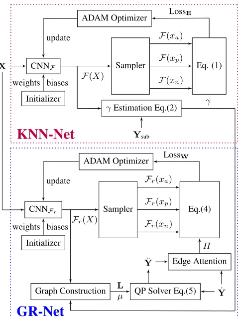
To solve the above deep metric learning problem we propose a deep graph regularized network (DGR-Net), shown in Fig. 1, comprising two sub-networks: (I) KNN-Net (deep metric learning-based KNN classifier): used to estimate the optimalγ, see (2), where an undi-rected KNN graph is constructed by learning a deep metric function through minimization ofLossE (1). (II) Graph-Net (graph-based binary classifier): used to learn edge weightsWvia (3) and (4) to construct a weighted undirected graph,G, constrained by the opti-malγ, to perform graph Laplacian regularization to obtain the solu-tionY¨ (5). To guarantee the solutionY¨ to (5) is numerically stable, we heuristically set conditional number,κ, as defined in [17], to 50 in all our experiments.

The proposed CNNs are shown in Fig. 2, which differ only in the loss function used: CNNFwithin KNN-Net uses edge loss (1),

while CNNFr weight loss (3), both trained via ADAM optimizer

with initial learning rate of 0.002 linearly decreasing with the num-ber of epochs. We use the same distance margin of 10 for bothαE andαWin (1, 3). For each epochs, we use batch size of 6, each batch comprising 120 nodes, thus we randomly sample6·120samples into the network. This results in 6 graphs to regularize the training.

Note that to achieve sparse, connected graph, we disconnect rel-atively low weighted edges that are most likely connecting incor-rectly labeled nodes. We adopt KNN-graph construction based on (2), where optimal maximum number of neighborsγis obtained via grid-search by evaluating classification error of an KNN-classifier on the validation set. The resultingγ is then used in the GR-Net

X CNNF

Initializer

Sampler Eq. (1) ADAM Optimizer

CNNFr

Initializer

γEstimation Eq.(2)

Ysub

weights biases

weights biases

ADAM Optimizer

Graph Construction QP Solver Eq.(5) _Y˙

F(X)

F(xa)

F(xp)

F(xn)

LossE

update

L

µ

Sampler Eq.(4)

γ

LossW

update

Fr(X)

Fr(xa)

Fr(xp)

Fr(xn)

¨

Y Edge Attention

Π

KNN-Net

GR-Net

Fig. 1:Overall block diagram of the proposed DGR-Net. KNN-Net first learns a deep metric function CNNFby minimizing LossE. We

adopt a Sampler to extract triplets:F(xa)- random instances inX,

F(xp)- random instance subsets ofXwith the same label asF(xa),

F(xn)- random instance subsets ofXwith the opposite label to

F(Xa). Once we obtainF∗

(·), we construct KNN graphs using (2) given a subset of training data (Xsub|Ysub) not used for minimizing

LossE, i.e.,Xsub ⊂ Xand Ysub ⊂ Y˙. An optimalγis then

es-timated by evaluating KNN classification accuracy on those KNN graphs where random subsets of nodes are manually unlabeled.γis then used as maximum degree of undirected KNN-graph constructed in the following GR-Net by minimizing LossW. GR-Net learns a regularized deep metric function CNNFrto assign edge weights and

constructs undirected KNN graphs constrained byγ. Then, it uses GLR to estimateY¨ givenY˙ via (5). Attention is then computed by an activation function to penalize LossW.

濈濊瀋濄

濄濉濓濈濈瀋濄

濄濉濓濅濊瀋濄

濄濅濋

濆濅 濖瀂瀁瀉

濆瀋濄 濄瀋濄

濃濩濨濤濩濨澮澔 !!"(#)

澽濢濤濩濨澮澔濌澔

濣瀂瀂濿 濅瀋濄 濅瀋濄

濙濖 濙濖

Fig. 2: CNNF and CNNF_r neural network. FC denotes fully

for pruning edge weightsWduring graph weighting. Like in [15], [17], we adopt Gaussian kernel as normalization functionP in (3) for assigning edge weightsWof graphG. OnceWis defined,Eis computed as a mask matrix for undirected KNN graph, where only topγentries{ei,j1, . . . , ei,jγ}of thei-th node are set to 1.

As mentioned in Sec. 3.2, we then solve the MAP problem (5), passing graph LaplacianLand partial labeled observationsY˙. In case of insufficient training data, edge attention activationΘ, im-plemented as a nonzero thresholded step as in (6), will be used to dropout some edges with relatively large changes betweenY¨ and originalY˙ after applying graph Laplacian regularization. This fa-cilitates to penalize learning on edges with relative low confidence (outliers). Therefore, the overall training regularizes CNNFr better

than typically dropout random neural units in the network.

Θ(Y¨,Y) =˙

(

1, if|_Y¨_−Y˙_{|> ε}

0, if|_Y¨_−Y˙_{| ≤ε,} (6)

where thresholdεis used to measure how confident a node’s label is and also helps to control the sparsity of edge attention matrixΠ. Un-der the assumption of ineffective graph Laplacian regularization dur-ing the early traindur-ing, we adopt a decayedεdecreasing linearly from 2 to 0.6 during training to ensure that we start regularizing CNNFr

until we obtain acceptable Laplacian matrixLwithout influence the earlier training.

4. RESULTS

In this section, we evaluate our proposed network benchmarked against different classifiers using classification error rate as perfor-mance metric. We select two binary-class datasets from Knowledge Extraction based on Evolutionary Learning dataset (KEEL) [32]: (1)

Phoneme: classification of nasal (class 0) and oral sounds (class 1), consisting of 5404 instances (frames) described by 5 phonemes of digitized speech. (2)Spambase: determining whether an email is spam (class 0) or not (class 1), with 4597 email messages summa-rized by 57 particular words or characters.

We compare the proposed DGC network against the following classifiers: (1) linear SVM (2) SVM with radial basis function ker-nel (denoted by SVM-RBF) (3) a purely graph-based classifier with smoothness prior (Graph) (4) a classical CNN, consisting of one CNN with two fully connected layers at the end; CNN block has a convolutional layer, a max pooling layer, and one dropout layer before each fully connected layer;l2regularization is applied to all

trainable layers (denoted by CNN) (5) a graph-based CNN with mul-tiple KNN graph construction blocks, which also learns the optimal graph structure as the proposed method but using edge convolution (denoted by DynGraph-CNN) [20]; batch normalization,l2

regular-ization and dropout are all used (6) a KNN classifier using deep met-ric learning [19] (DML-KNN) withl2regularization and dropout.

We conduct our experiments by randomly splitting each dataset into training, validation and testing sets. We select 10, 15, 20, 25, 30% of instances as training sets, 10%, instances as validation set, and the remaining instances contribute towards the testing set. Clas-sification error rates are measured by running 20 experiments for each dataset. We use the same random seed setting across all clas-sification methods and remove all duplicated instances to ensure a fair comparison. Hyper-parameters used for each experiment are obtained from the validation set by grid search.

As shown in Tables 1 & 2, given insufficient amount of data, DGC consistently outperforms the other 6 benchmarks, as observed by lower classification error rates. One reason is that all other neu-ral network-based classifiers overfit to the insufficient training data. Indeed, the proposed method uniformly outperforms all benchmarks

Table 1:Classification Error Rate (%) for the Phoneme Dataset for various sizes of the training dataset expressed as the proportion of the total dataset (%).

Proportion (%) 10 15 20 25 30

SVM-Linear 25.73 25.79 25.62 25.63 25.60 SVM-RBF 20.81 20.32 19.78 19.45 19.05 Graph 23.09 22.92 22.72 22.34 22.17 CNN 20.69 20.22 19.51 19.12 18.91 DynGraph-CNN 22.12 20.20 19.39 19.21 18.40 DML-KNN 20.37 19.44 19.31 19.18 18.12

DGC 19.86 19.37 18.93 18.78 17.89

Table 2:Classification Error Rate (%) for the Spambase Dataset for various sizes of the training dataset expressed as the proportion of the total dataset (%).

Proportion (%) 10 15 20 25 30

SVM-Linear 10.26 9.83 9.52 9.06 8.94 SVM-RBF 10.04 9.30 9.00 8.61 8.41 Graph 20.22 20.10 19.68 19.13 18.72

CNN 9.72 9.18 8.75 8.65 8.26

DynGraph-CNN 11.84 10.71 9.52 9.38 9.09 DML-KNN 9.20 8.26 7.97 7.73 7.44

DGC 9.08 8.18 7.64 7.52 7.38

for the training dataset sizes between 10%-30% of the total dataset. The Graph method, based on graph Laplacian regularization, does not learn features, resulting in the worst performance among all tested schemes. DynGraph-CNN network [20] performs worse than CNN when the amount of training data is very low, since the network is deeper than the CNN benchmark, closing the performance gap as the training dataset size increases. DML-KNN is always the sec-ond best method indicating that learning deep metric via triplet loss provides performance gain. Further improvements of the proposed DGC over DML-KNN are due to the effectiveness of the proposed graph Laplacian regularization.

5. CONCLUSIONS

A deep graph regularized network architecture for binary classifier learning for the case of insufficient training data is proposed and benchmarked against classical and state-of-the-art classifiers. The proposed solution embeds graph Laplacian regularization, a proven method to combat insufficient training dataset, into a CNN archi-tecture used for deep feature learning via new formulation of a loss function that takes into account the quality of the underlying graph used to calculate the graph Laplacian. The proposed network consis-tently outperforms six benchmarks, including a prior graph Lapla-cian regularization approach, conventional CNN and SVM classi-fiers, as well as latest state-of-the-art dynamic graph CNN architec-ture that uses geometric learning to find optimal graph strucarchitec-ture.

Future work will comprise extending the work to handle noise in the training dataset. Another direction is extending the work to the multi-class classification problem.

6. ACKNOWLEDGMENT

References

[1] A. Krizhevsky, I. Sutskever, and G. E. Hinton, “Imagenet classification with deep convolutional neural networks,” in Advances in neural information processing systems, 2012, pp. 1097–1105.

[2] A. Graves, A.-R. Mohamed, and G. Hinton, “Speech recog-nition with deep recurrent neural networks,” inICASSP 2013, 2013, pp. 6645–6649.

[3] Y. Xu, T. Mo, Q. Feng, P. Zhong, M. Lai, and E. I. Chang, “Deep learning of feature representation with multiple in-stance learning for medical image analysis,” in ICASSP-2014, May ICASSP-2014, pp. 1626–1630.

[4] J. Kukaˇcka, V. Golkov, and D. Cremers, “Regularization for deep learning: A taxonomy,”ArXiv:1710.10686, 2017. [5] L. Perez and J. Wang, “The effectiveness of data

aug-mentation in image classification using deep learning,” ArXiv:1712.04621, 2017.

[6] A. Mikołajczyk and M. Grochowski, “Data augmentation for improving deep learning in image classification problem,” in 2018 IIPhDW, May 2018, pp. 117–122.

[7] G. E. Hinton, N. Srivastava, A. Krizhevsky, I. Sutskever, and R. R. Salakhutdinov, “Improving neural networks by prevent-ing co-adaptation of feature detectors,” ArXiv:1207.0580, 2012.

[8] K. He, X. Zhang, S. Ren, and J. Sun, “Deep residual learning for image recognition,” inPro.e IEEE Conf. Computer Vision and Pattern Recognition, 2016, pp. 770–778.

[9] G. Huang, Z. Liu, L. Van Der Maaten, and K. Q. Weinberger, “Densely connected convolutional networks.,” in CVPR, vol. 1, 2017, p. 3.

[10] A. C. Wilson, R. Roelofs, M. Stern, N. Srebro, and B. Recht, “The marginal value of adaptive gradient methods in machine learning,” inAdvances in Neural Information Processing Sys-tems, 2017, pp. 4148–4158.

[11] F. Milletari, N. Navab, and S.-A. Ahmadi, “V-net: Fully convolutional neural networks for volumetric medical image segmentation,” in2016 Fourth Intl. Conf. 3D Vision (3DV), IEEE, 2016, pp. 565–571.

[12] A. Ortega, P. Frossard, J. Kovacevic, J. M. F. Moura, and P. Vandergheynst, “Graph signal processing: Overview, challenges, and applications,” in Proceedings of the IEEE, vol. 106, no.5, May 2018, pp. 808–828.

[13] A. Sandryhaila and J. M. F. Moura, “Classification via reg-ularization on graphs,” in2013 IEEE Global Conference on Signal and Information Processing, Dec. 2013, pp. 495–498. [14] J. Pang and G. Cheung, “Graph Laplacian regularization for image denoising: Analysis in the continuous domain,”IEEE Transactions on Image Processing, vol. 26, no. 4, pp. 1770– 1785, 2017.

[15] G. Cheung, W. Su, Y. Mao, and C. Lin, “Robust semisuper-vised graph classifier learning with negative edge weights,” IEEE Transactions on Signal and Information Processing over Networks, vol. 4, no. 4, pp. 712–726, Dec. 2018.

[16] C. Yang, G. Cheung, and V. Stankovic, “Alternating binary classifier and graph learning from partial labels,” in Asia-Pacific Signal and Information Processing Association An-nual Summit and Conference 2018, Nov. 2018.

[17] J. Zeng, J. Pang, W. Sun, and G. Cheung, “Deep graph Laplacian regularization for robust denoising of real im-ages,”ArXiv 1807.11637, 2018.

[18] C. Cortes and V. Vapnik, “Support-vector networks,” Ma-chine learning, vol. 20, no. 3, pp. 273–297, 1995.

[19] E. Hoffer and N. Ailon, “Deep metric learning using triplet network,” in International Workshop on Similarity-Based Pattern Recognition, Springer, 2015, pp. 84–92.

[20] Y. Wang, Y. Sun, Z. Liu, S. E. Sarma, M. M. Bronstein, and J. M. Solomon, “Dynamic graph CNN for learning on point clouds,”ICLR 2017, vol. abs/1801.07829, 2018.

[21] M. M. Bronstein, J. Bruna, Y. LeCun, A. Szlam, and P. Vandergheynst, “Geometric deep learning: Going beyond euclidean data,”IEEE Signal Processing Magazine, vol. 34, no. 4, pp. 18–42, Jul. 2017.

[22] T. N. Kipf and M. Welling, “Semi-supervised classifica-tion with graph convoluclassifica-tional networks,”ArXiv:1609.02907, 2016.

[23] F. Scarselli, M. Gori, A. C. Tsoi, M. Hagenbuchner, and G. Monfardini, “The graph neural network model,”IEEE Trans-actions on Neural Networks, vol. 20, no. 1, pp. 61–80, Jan. 2009.

[24] J. Bruna, W. Zaremba, A. Szlam, and Y. LeCun, “Spec-tral networks and locally connected networks on graphs,” ArXiv:1312.6203, 2013.

[25] M. Defferrard, X. Bresson, and P. Vandergheynst, “Convolu-tional neural networks on graphs with fast localized spectral filtering,” inAdvances in Neural Information Processing Sys-tems 29, Curran Associates, Inc., 2016, pp. 3844–3852.

[26] X. Zhang, C. Xu, and D. Tao, “Graph edge convolutional neural networks for skeleton based action recognition,” ArXiv:1805.06184, 2018.

[27] D. I. Shuman, S. K. Narang, P. Frossard, A. Ortega, and P. Vandergheynst, “The emerging field of signal processing on graphs: Extending high-dimensional data analysis to net-works and other irregular domains,”IEEE Signal Processing Magazine, vol. 30, no. 3, pp. 83–98, May 2013.

[28] F. Schroff, D. Kalenichenko, and J. Philbin, “Facenet: A uni-fied embedding for face recognition and clustering,” in Pro-ceedings of the IEEE Conf. Computer Vision and Pattern Recognition, 2015, pp. 815–823.

[29] A. Hermans, L. Beyer, and B. Leibe, “In defense of the triplet loss for person re-identification,”ArXiv:1703.07737, 2017.

[30] G. L. Miller, S.-H. Teng, W. Thurston, and S. A. Vava-sis, “Separators for sphere-packings and nearest neighbor graphs,”Journal of the ACM, vol. 44, no. 1, pp. 1–29, 1997.

[31] P. Lemberger, “On generalization and regularization in deep learning,”ArXiv:1704.01312, 2017.